This document describes the steps for performing multiple logistic regression analysis. It outlines introducing logistic regression and its advantages over linear regression for binary outcomes. It then details the steps of multiple logistic regression analysis, including descriptive statistics, variable selection, model fit assessment, and final model interpretation. Variable selection involves univariable and multivariable analyses to identify significant predictors. Model fit is assessed using Hosmer-Lemeshow test, classification table, and AUC. The example analysis identifies diastolic blood pressure and gender as significant predictors of coronary artery disease.

1. 1
Multiple LogisticRegression
14Dec 2015 Intermediate Statistics IPS
Dott. Ric. Sara A.
Professor of Inorganic chemistry;
Member, Research Advisory Council;
Università degli Studi di Padova,italy.
For lecture’s copy in Italian please contact Sig.Alessandro Patanè at the end of lecture.
Difficulty Level: Intermediate

2. Outlines
2
●
●
Introduction
Stepsin Multiple LogisticRegression
1.Descriptive Statistics
2.Variable Selection
3.Model FitAssessment
4.Final Model Interpretation& Presentation
For lecture’s copy in Italian please contact Sig.Alessandro Patanè at the end of lecture.

3. Objectives
3
1.Understand the reasonsbehind theuseof logistic
regression.
2.Perform multiple logistic regressionin SPSS.
3.Identify and interpret the relevantSPSSoutputs.
4.Summarize important results in atable.
For lecture’s copy in Italian please contact Sig.Alessandro Patanè at the end of lecture.

4. Introduction
4
●
●
●
●
Logistic regression isusedwhen:
– Dependent Variable, DV:Abinary categoricalvariable
[Yes/No], [Disease/No disease] i.e the outcome.
Simple logistic regression –Univariable:
– Independent Variable, IV:Acategorical/numerical variable.
Multiple logistic regression –Multivariable:
– IVs:Categorical & numericalvariables.
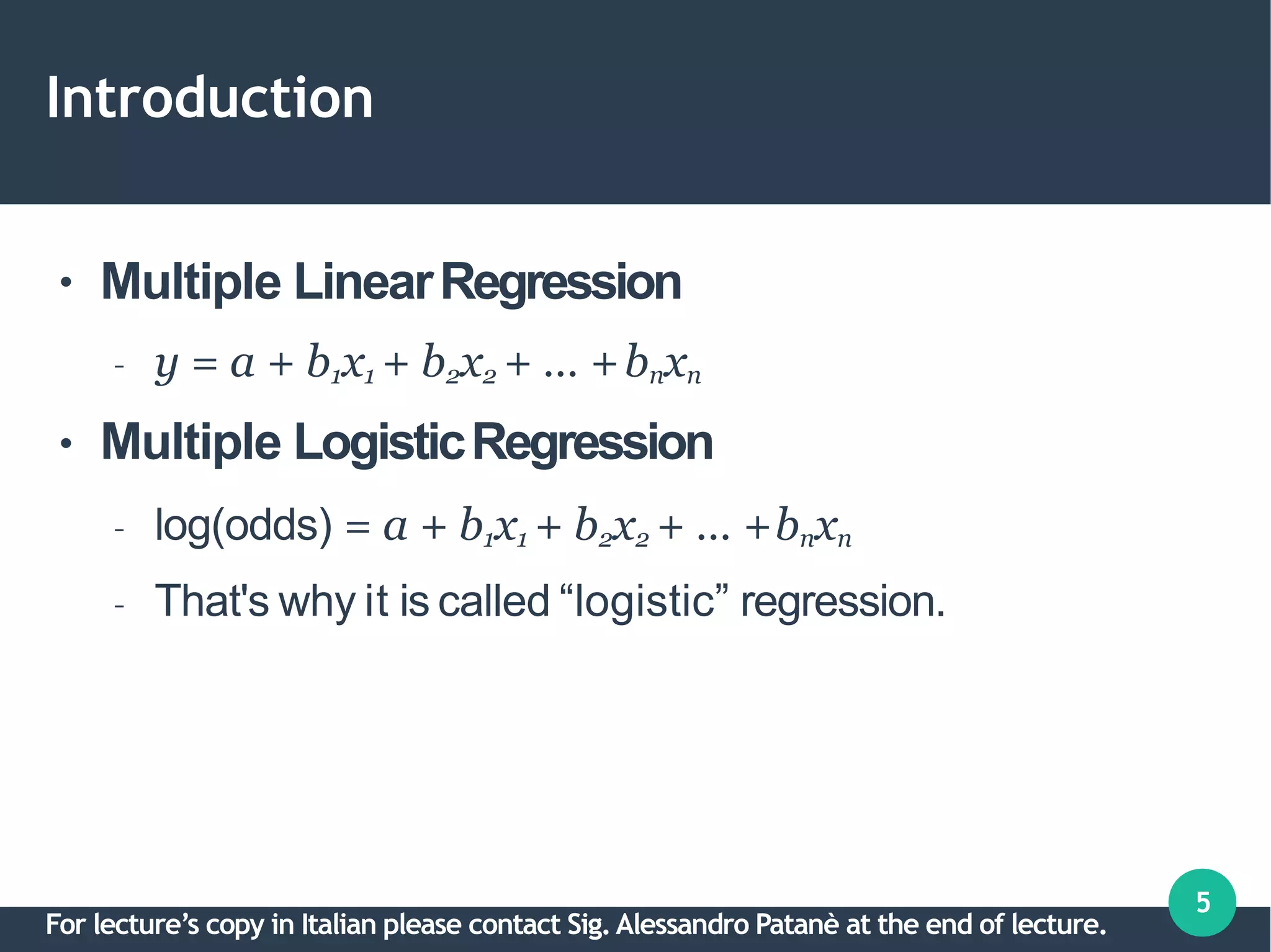
Recall –Multiple LinearRegression?
For lecture’s copy in Italian please contact Sig.Alessandro Patanè at the end of lecture.

5. Introduction
5
●
●
Multiple LinearRegression
– y = a + b1x1 + b2x2 + … +bnxn
Multiple LogisticRegression
– log(odds) = a + b1x1 + b2x2 + … +bnxn
– That's why it is called “logistic” regression.
For lecture’s copy in Italian please contact Sig.Alessandro Patanè at the end of lecture.

6. Introduction
6
●
●
●
Binary outcome: Concerned with OddsRatio.
– Oddsis a measure of chance like probability.
– Odds =n(Disease)/n(no Disease) among agroup.
– Odds Ratio, OR=Odds(Factor)/Odds(No factor)
– Applicable to all observational study designs.
Relative Risk,RR
– Only cohort study.
OR≈ RRfor rare disease, useful to determinerisk.
For lecture’s copy in Italian please contact Sig.Alessandro Patanè at the end of lecture.

7. Introduction
7
●
●
●
●
Odds(man) =a/b =24/76 =0.32
Odds(woman) =c/d =13/87 =0.15
OR(man/woman) =0.32/0.15 =2.13
Shortcut, OR=ad/bc =(24x87)/(76x13) =2.11
Factor vs CAD CAD No CAD
Man 24 [a] 76 [b]
Woman
(i.e. not Man)
13 [c] 87 [d]
For lecture’s copy in Italian please contact Sig.Alessandro Patanè at the end of lecture.

8. Introduction
8
●
●
●
Risk(man) =Proportion CAD=a/(a+b) =0.24
Risk(woman) =Proportion CADc/(c+d) =0.13
RR(man/woman) =0.24/0.13 =1.85 ≈ OR,2.11
Factor vs CAD CAD No CAD
Man 24 [a] 76 [b]
Woman
(i.e. not Man)
13 [c] 87 [d]
For lecture’s copy in Italian please contact Sig.Alessandro Patanè at the end of lecture.

9. Steps in Multiple Logistic Regression
9
●
●
●
●
Dataset: slog.sav
Sample size, n=200
DV:cad (1: Yes,0:No)
IVs:
– Numerical: sbp (systolic blood pressure), dbp (diastolic
blood pressure), chol (serum cholesterol in mmol/L), age
(age in years), bmi (Body MassIndex).
– Categorical: race (0: Malay, 1: Chinese, 2: Indian), gender (0:
Female, 1:Male)
For lecture’s copy in Italian please contact Sig.Alessandro Patanè at the end of lecture.

10. Steps in Multiple Logistic Regression
1.Descriptivestatistics.
2.Variable selection.
a.Univariable analysis.
b.Multivariable analysis.
c.Multicollinearity.
d.Interactions.
3.Model fit assessment.
4.Final model interpretation &presentation.
For lecture’s copy in Italian please contact Sig.Alessandro Patanè at the end of lecture.

11. 1. Descriptivestatistics
● Set outputs byCAD
status.
– Data → Split File
→ Select Compare
groups
– Set Groups Based
on:
cad, OK
For lecture’s copy in Italian please contact Sig.Alessandro Patanè at the end of lecture.

12. 1. Descriptivestatistics
● Obtain mean(SD)
and n(%) by CAD
group.
– Analyze →
Descriptive
Statistics →
Frequencies
– Include relevant
variables in
Variables
For lecture’s copy in Italian please contact Sig.Alessandro Patanè at the end of lecture.

13. 1. Descriptivestatistics
● Cont...
– Statistics →
tick →
Continue
For lecture’s copy in Italian please contact Sig.Alessandro Patanè at the end of lecture.

14. 1. Descriptivestatistics
● Cont...
– Charts →
tick →
Continue
→ OK
For lecture’s copy in Italian please contact Sig.Alessandro Patanè at the end of lecture.

15. 1. Descriptivestatistics
● Results
For lecture’s copy in Italian please contact Sig.Alessandro Patanè at the end of lecture.

16. 1. Descriptivestatistics
● Results
For lecture’s copy in Italian please contact Sig.Alessandro Patanè at the end of lecture.

17. 1. Descriptivestatistics
●
●
Results
– Lookat histogramsto decide
data normalityfor numerical
variables. Rememberyour
BasicStats!
Caution! Reset back the
data.
– Data → Split File →
Select
Analyze all cases
– OK
For lecture’s copy in Italian please contact Sig.Alessandro Patanè at the end of lecture.

18. 1. Descriptivestatistics
● Present the results in a table.
Factors
CAD,n=37
mean(SD)
NoCAD,n=163
mean(SD)
Systolic BloodPressure 143.8(25.61) 129.3(22.26)
Diastolic BloodPressure 89.0(12.17) 80.8(12.61)
Cholesterol 6.6(1.17) 6.1(1.17)
Age 47.4(8.80) 45.2(8.41)
BMI 36.4(3.99) 36.9(3.77)
Race*
Malay
Chines
e
Indian
13(35.1%)
12(32.4%)
12(32.4%)
60(36.8%)
52(31.9%)
51(31.3%)
Gender*
Male
Femal
e
24(64.9%)
13(35.1%)
76(46.6%)
87(53.4%)
For lecture’s copy in Italian please contact Sig.Alessandro Patanè at the end of lecture.

19. 2. Variableselection
● To select best variables to predict the
outcome.
• Sub-steps:
a.Univariable analysis.
b.Multivariable analysis.
c.Checking multicollinearity & interactions.
For lecture’s copy in Italian please contact Sig.Alessandro Patanè at the end of lecture.

20. 2a. Univariableanalysis
●
●
Perform Simple Logistic Regression on
each IV. Select IVs which fullfill:
– P-value < 0.25 → Statistical significance.
– Clinically significant IVs → You decide.
For lecture’s copy in Italian please contact Sig.Alessandro Patanè at the end of lecture.

21. 2a. Univariableanalysis
● Analyze numerical
variables:
– Analyze → Regression
→
Binary Logistic
– Dependent: cad,
Covariates: sbp
– Click Options → Tick
Iteration history, CI
for exp(B) →
Continue → OK
– Repeat for dbp, chol, age,
bmi
For lecture’s copy in Italian please contact Sig.Alessandro Patanè at the end of lecture.

22. 2a. Univariableanalysis
● Results
Model: SBP P-
value=0.001 by
Likelihood Ratio
(LR) test
SBP P-value=0.001
by Wald test
●
●
●
●
Exp(B) is OR.
OR(1 unit ↑ in SBP)
=1.04(95% CI: 1.01,
1.04). Unadjusted/
Crude OR.
Interpretation:
1mmHg increase in
SBP increase odds of
CAD by 1.02 times.
In variable selection
context, less concern
about OR &
interpretation.
For lecture’s copy in Italian please contact Sig.Alessandro Patanè at the end of lecture.

23. 2a. Univariableanalysis
● Analyze categorical
variables:
– Dependent: cad,
Covariates: gender
– Click Categorical →
Categorical Covariates:
gender → Change Contrast
→ Reference Category:
First → Change →
Continue.
– Repeat for race
For lecture’s copy in Italian please contact Sig.Alessandro Patanè at the end of lecture.

24. 2a. Univariableanalysis
● Results Women=0
becomes the
reference group.
Model: Gender P-
value=0.044 by LR test
Gender P-value=0.048
by Wald test
●
●
OR(male)=2.11(95
% CI: 1.01, 4.44).
Unadjusted/Crud
e OR.
Interpretation:
Man has 2.11
times odds of
CAD as compared
to woman.
For lecture’s copy in Italian please contact Sig.Alessandro Patanè at the end of lecture.

25. 25
2a. Univariableanalysis
● P-values of IVs – select P-value < 0.25
Factors P-value(Waldtest) P-value(LRtest)
Systolic BloodPressure 0.001 0.001
Diastolic BloodPressure 0.001 0.001
Cholesterol 0.012 0.011
Age 0.143 0.141
BMI 0.505 0.511
Race
Chinese-vs-
Malay Indian-
vs-Malay
0.887
0.852
0.981*
Gender Man-Woman 0.048 0.044
*For bothvariables
For lecture’s copy in Italian please contact Sig.Alessandro Patanè at the end of lecture.

26. 2b. Multivariableanalysis
●
●
●
●
Selected variables:
– sbp, dbp, chol, age, gender
Perform Multiple logistic regression of the
selected variables (multivariable) in on go.
Variable selection is now proceed at
multivariable level.
Some may remain significant, some
become insignificant.
For lecture’s copy in Italian please contact Sig.Alessandro Patanè at the end of lecture.

27. 2b. Multivariableanalysis
● VariableSelection
Methods:
– Automatic.
●
●
Forward: Conditional,LR,
Wald. Entersvariables.
Backward: Conditional,LR,
Wald. Removesvariables.
– Manual.
● Enter. Entry & removal of
variables done manually.
(Recommended, butleave to
experts/statisticians).
For lecture’s copy in Italian please contact Sig.Alessandro Patanè at the end of lecture.

28. 2b. Multivariableanalysis
● Variable Selection in thisworkshop:
– Automatic by Forward &Backward LR.
– Selection of variables by P-values based on LRtest.
For lecture’s copy in Italian please contact Sig.Alessandro Patanè at the end of lecture.

29. 2b. Multivariableanalysis
●
●
Enter all selectedvariables.
Perform 2x –1x Forward LR,1x BackwardLR.
Options:Just leave at the default values.
For lecture’s copy in Italian please contact Sig.Alessandro Patanè at the end of lecture.

30. 2b. Multivariableanalysis
● Results
Forward LR
Backward LR
●
●
Both methods
keep same
IVs:dbp &
gender.
P-valuesby
Waldtest.
For lecture’s copy in Italian please contact Sig.Alessandro Patanè at the end of lecture.

31. 2b. Multivariableanalysis
● Results
Backward LR
●
●
Both methods keep
same IVs: dbp &
gender.
P-values by LR test.
Forward LR
For lecture’s copy in Italian please contact Sig.Alessandro Patanè at the end of lecture.

32. 2c.Multicollinearity
●
●
●
Indicates redundant variables–
highly correlatedIVs.
Perform Enter method withdbp &
gender.
Lookat coefficients (B) &std
errors (SE) / ORs(95% CIs)if they
are suspiciouslylarge.
● Results
●
●
●
SEsare quitesmall
relative toBs.
95%CIsare nottoo
wide.
Nomulticollinearity.
For lecture’s copy in Italian please contact Sig.Alessandro Patanè at the end of lecture.

33. 2d. Interactions
●
●
IVscombination that
necessitates interpretation
of regressionseparately
based on levels of IV →
making thingscomplicated.
Perform Enter methodwith
dbp, gender &dbpxgender.
Select both dbp &gender
(hold Ctrl on keyboard) →
Click >a*b>
For lecture’s copy in Italian please contact Sig.Alessandro Patanè at the end of lecture.

34. 2d. Interactions
● Results
Wald test for dbp by gender
(dbp*gender) not sig. Can
remove the interaction term
from model.
For lecture’s copy in Italian please contact Sig.Alessandro Patanè at the end of lecture.

35. 2. Variableselection
● Atthe end of Variable SelectionStep →Preliminary
FinalModel.
P-values by LR per
variable. Obtained with
Forward LR method.
●
●
P-values by Wald
test per variable
by Enter method.
Take this adjusted
OR.
P-values by LR test for
both dbp & gender by
Enter method.
For lecture’s copy in Italian please contact Sig.Alessandro Patanè at the end of lecture.

36. 3. Model fitassessment
●
●
By these 3 goodness-of-fit assessment
methods:
a.Hosmer-Lemeshow test
b.Classification table.
c.Area under Receiver Operating Characteristics
(ROC) curve.
At the end → Final Model.
For lecture’s copy in Italian please contact Sig.Alessandro Patanè at the end of lecture.

37. 3. Model fitassessment
●
●
Perform Enter method with
dbp & gender.
Additionally
– Click Options... → Tick
Hosmer-Lemeshow
goodness-of-fit
– Click Save… → Tick
Probabilities under
Predicted Values
– A new variable PRE_1 will be
created.
For lecture’s copy in Italian please contact Sig.Alessandro Patanè at the end of lecture.

38. 3a. Hosmer-Lemeshowtest
● Indicates fit of Preliminary Final Model to data.
● Result
s
P-value 0.09 > 0.05 →
Good model fit to the data.
Observed counts in data.
●
●
Expected/predicted counts
by model.
The smaller the differences
between Observed vs
Expected → Better model fit
to data.
For lecture’s copy in Italian please contact Sig.Alessandro Patanè at the end of lecture.

39. 3b. Classificationtable
●
●
CAD & No CAD subjects observed vs
predicted/classified by Preliminary Final Model.
% correctly classified > 70% is expected for good
●
model fit.
Results ●
●
80% of subjects are
correctly classified by
the model.
Good model fit to the
data.
For lecture’s copy in Italian please contact Sig.Alessandro Patanè at the end of lecture.

40. 3c. Area under ROC curve (AUC)
●
●
●
●
A measure of ability of the model to
discriminate CAD vs Non CAD
subjects.
AUC > 0.7 is acceptable fit.
AUC ≤ 0.5 no discrimination at all,
not acceptable.
Steps
– Analyze → ROC curve... → Assign
Test Variable: Predicted probability
(PRE_1), State Variable: cad, Value
of State Variable: 1.
– Under Display tick ROC Curve, With
diagonal reference line and
Standard Error and confidence
interval.
For lecture’s copy in Italian please contact Sig.Alessandro Patanè at the end of lecture.

41. 3c. Area under ROC curve (AUC)
● Results
●
●
●
●
AUC=0.73 > 0.7.
95% CI: 0.64, 0.82.
Lower limit slightly < 0.7, still
acceptable > 0.5.
Good model fit to the data.
For lecture’s copy in Italian please contact Sig.Alessandro Patanè at the end of lecture.

42. 3. Model fitassessment
●
●
All 3 methods indicate good model fit of
Preliminary Final Model.
Can conclude the model with dbp & gender → Final
Model.
For lecture’s copy in Italian please contact Sig.Alessandro Patanè at the end of lecture.

43. 2. Final Model interpretation & presentation
● The Final Model.
P-values by LR per
variable. Obtained with
Forward LR method.
●
●
P-values by Wald
test per variable
by Enter method.
Take this adjusted
OR.
P-values by LR test for
both dbp & gender by
Enter method.
For lecture’s copy in Italian please contact Sig.Alessandro Patanè at the end of lecture.

44. 4. Final Model interpretation & presentation
● Associated factors of coronary artery disease.
a
LR test
Factors b Adjusted OR (95%
CI)
P-valuea
Diastolic Blood Pressure 0.05 1.05 (1.02, 1.08) < 0.001
Gender Man vs Woman 0.81 2.24 (1.04, 4.82) 0.036
1mmHg increase in DBP
increase odds of CAD
by 1.05 times, while
controlling for gender.
Man has 2.24 times odds of
CAD as compared to woman,
while controlling for DBP.
To obtain for 10mmHg increase in DBP
OR = exp(c x b) = exp(10 x 0.05) = exp(0.5) = 1.65 times.
For lecture’s copy in Italian please contact Sig.Alessandro Patanè at the end of lecture.

45. Q&A
For lecture’s copy in Italian please contact Sig.Alessandro Patanè at the end of lecture.