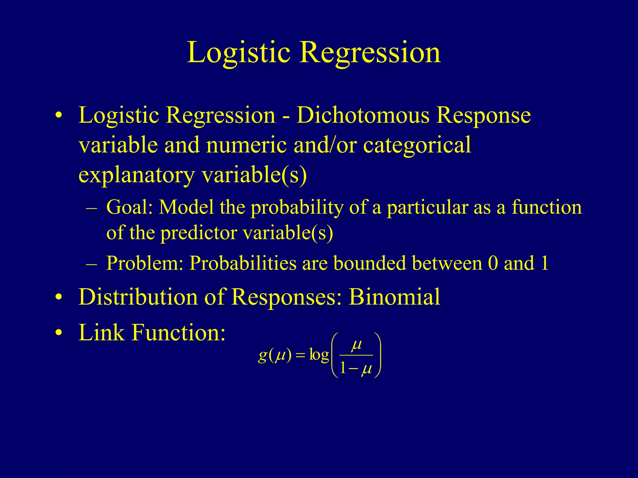
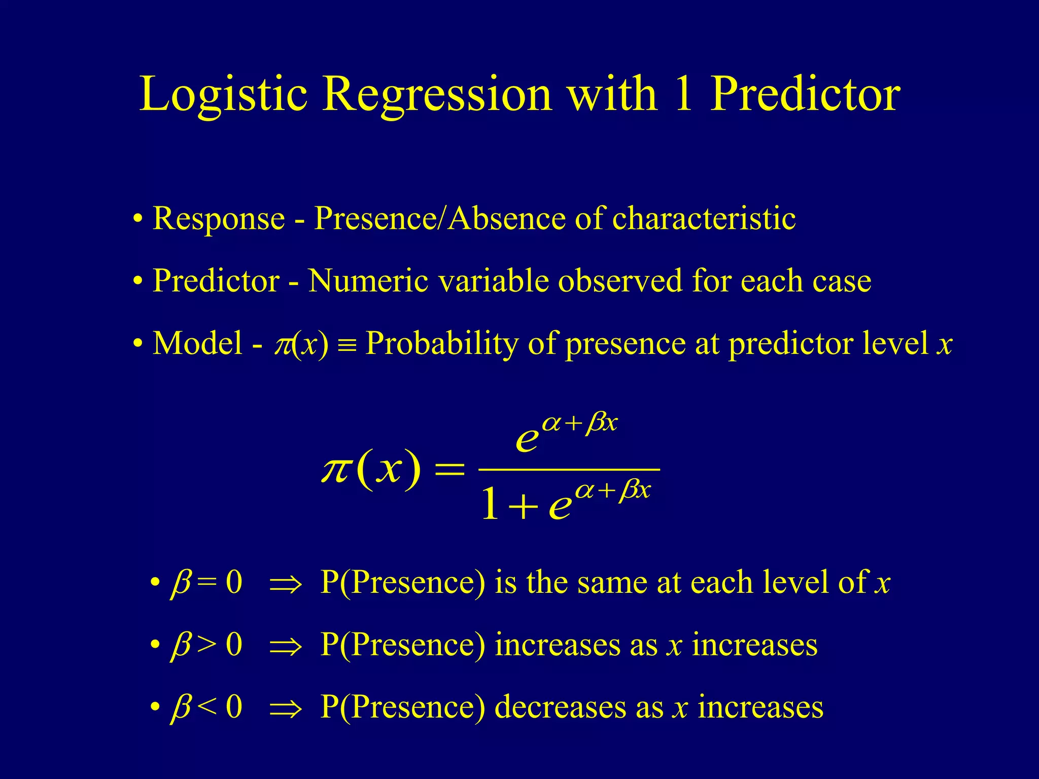
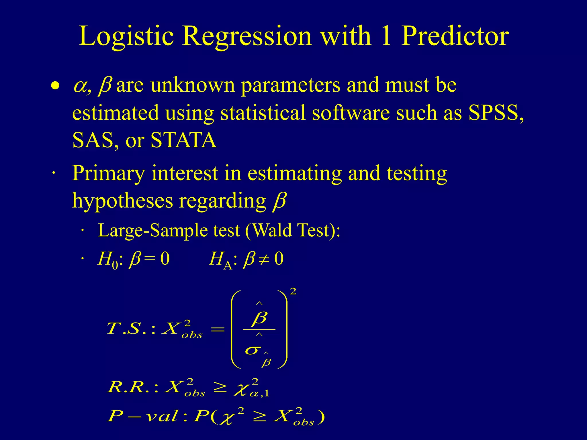
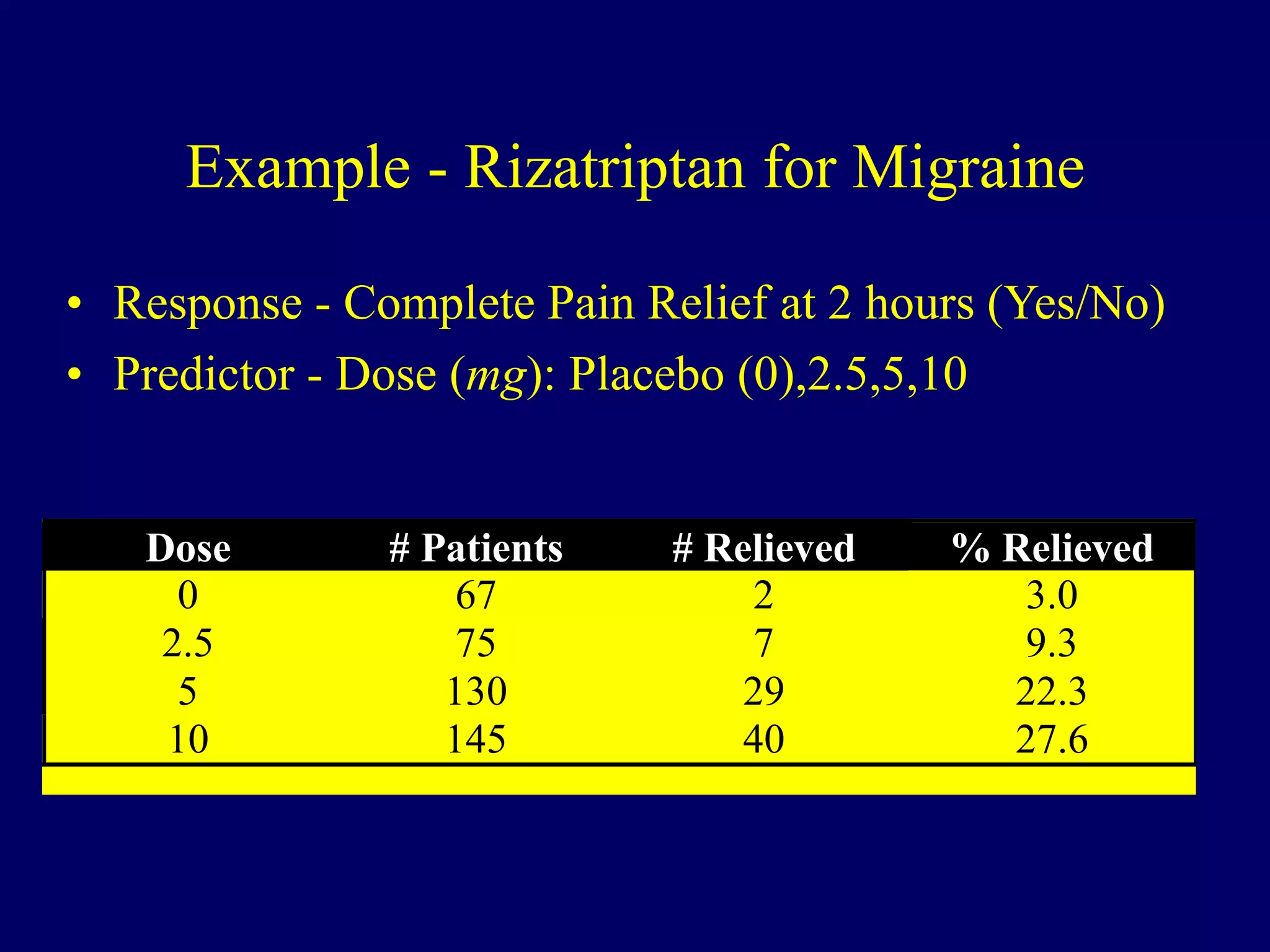
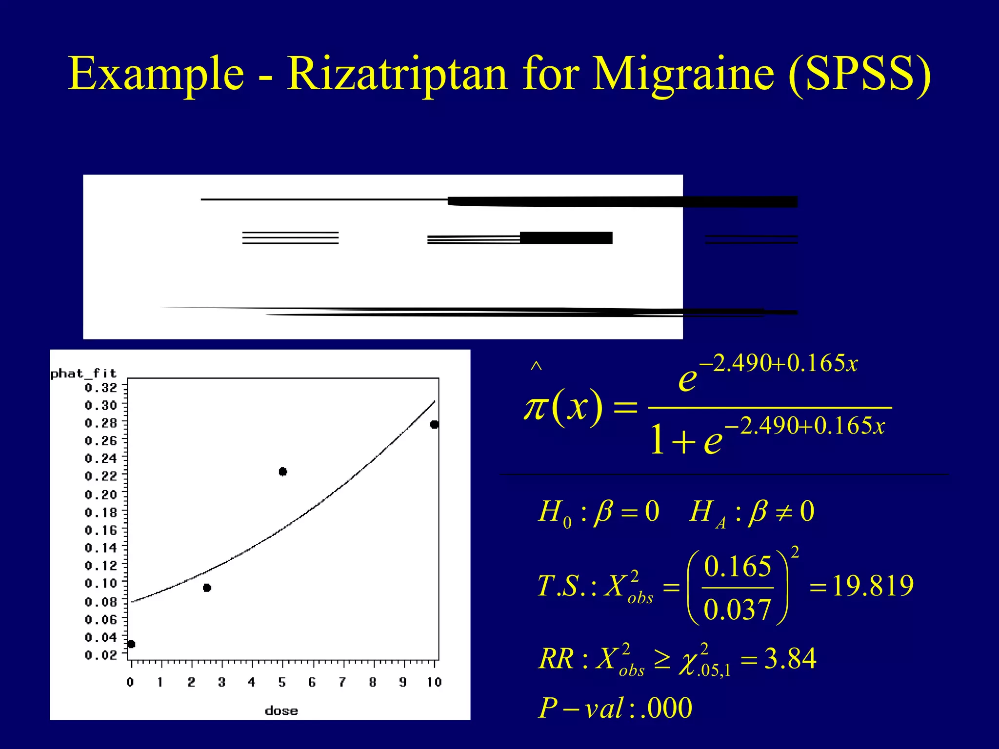
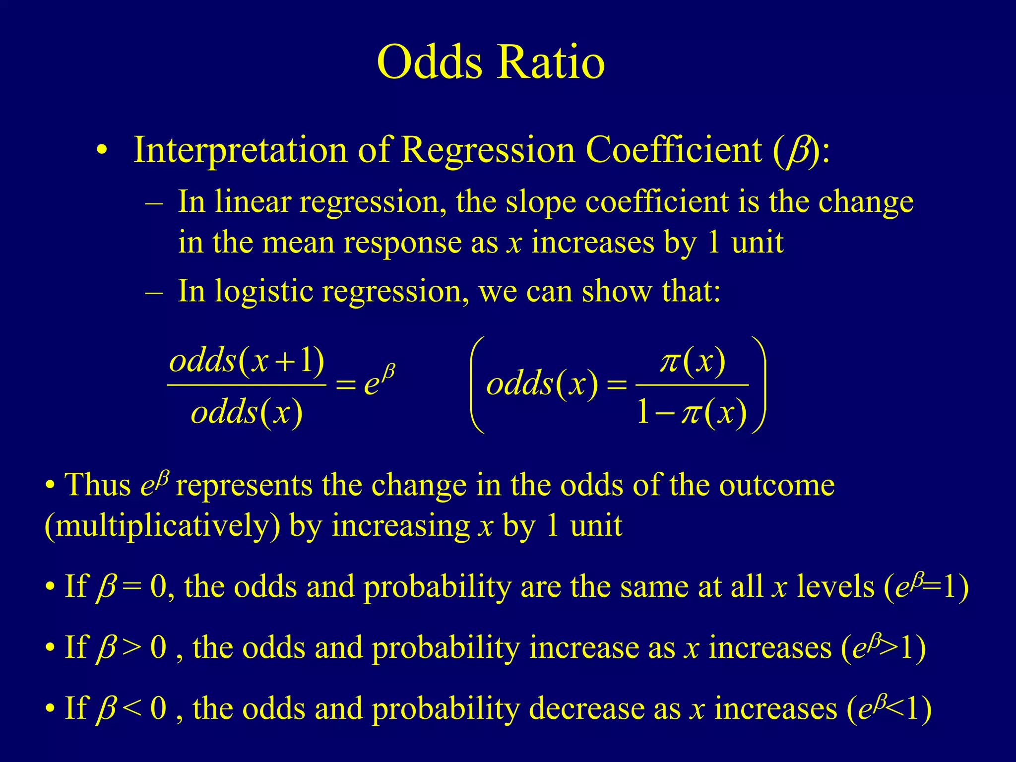
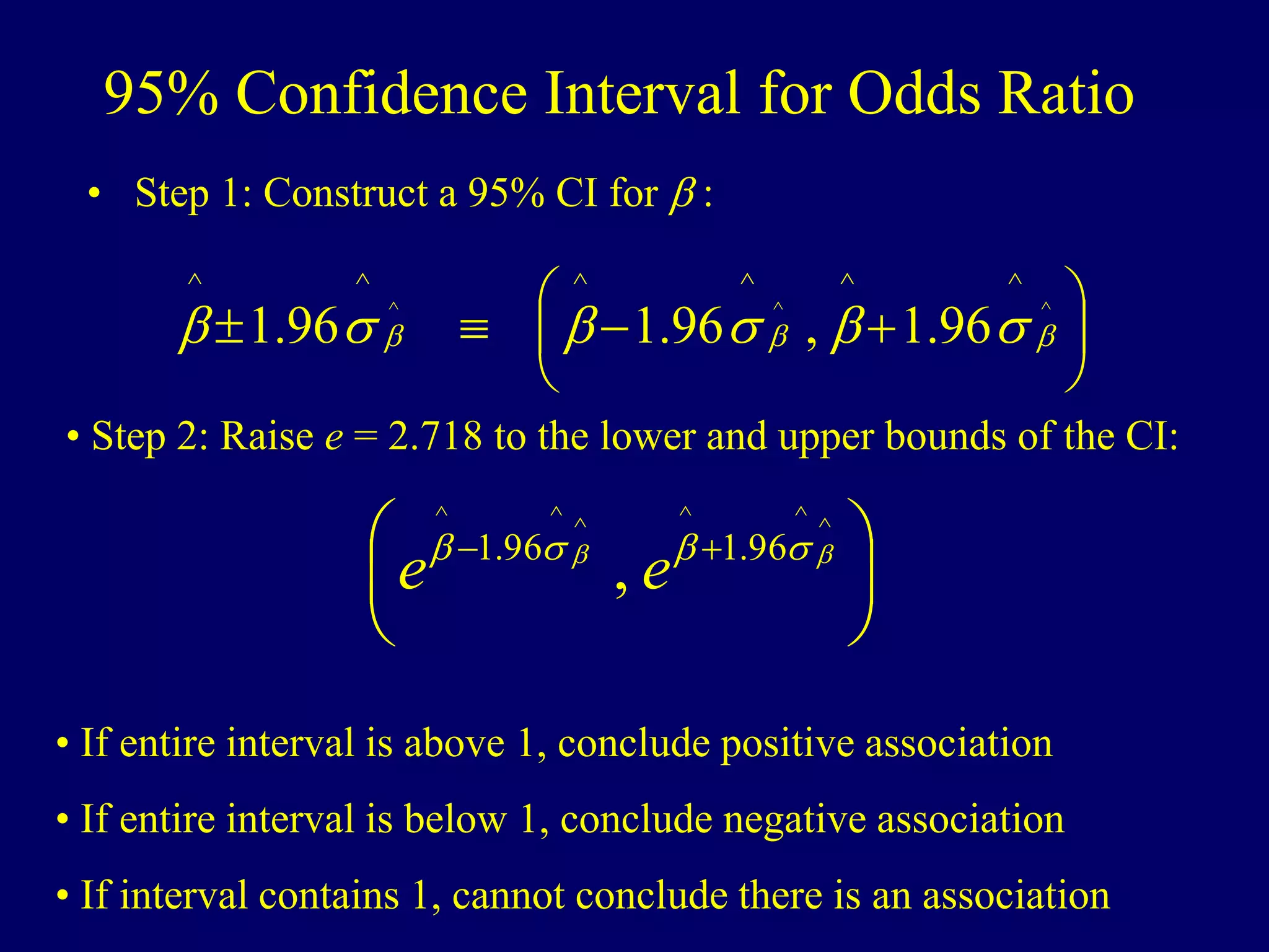
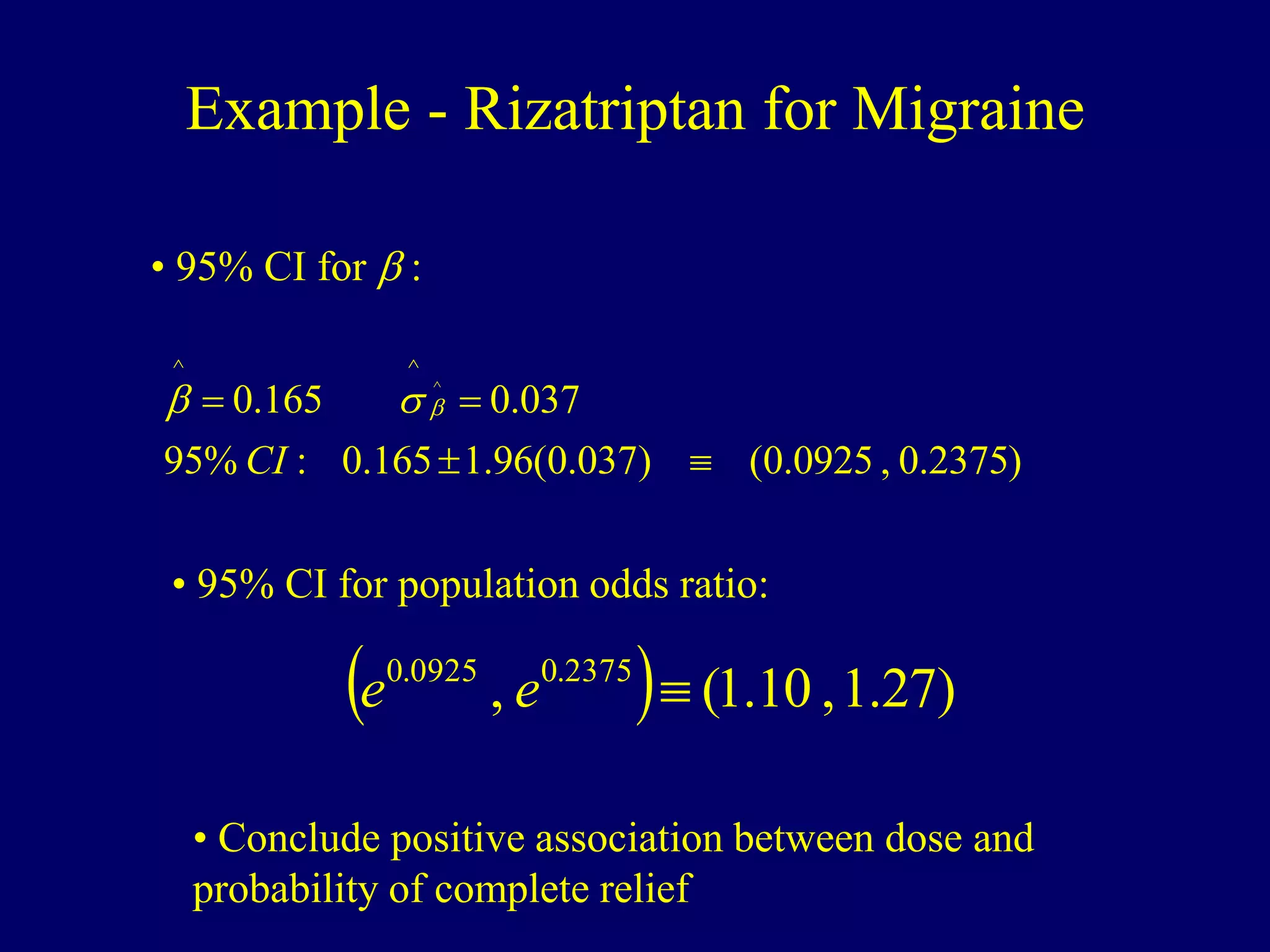
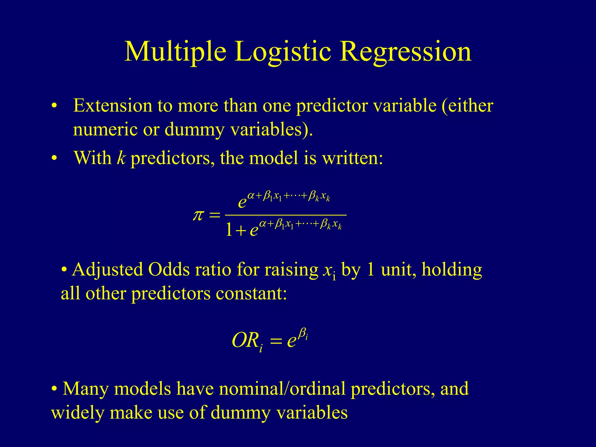
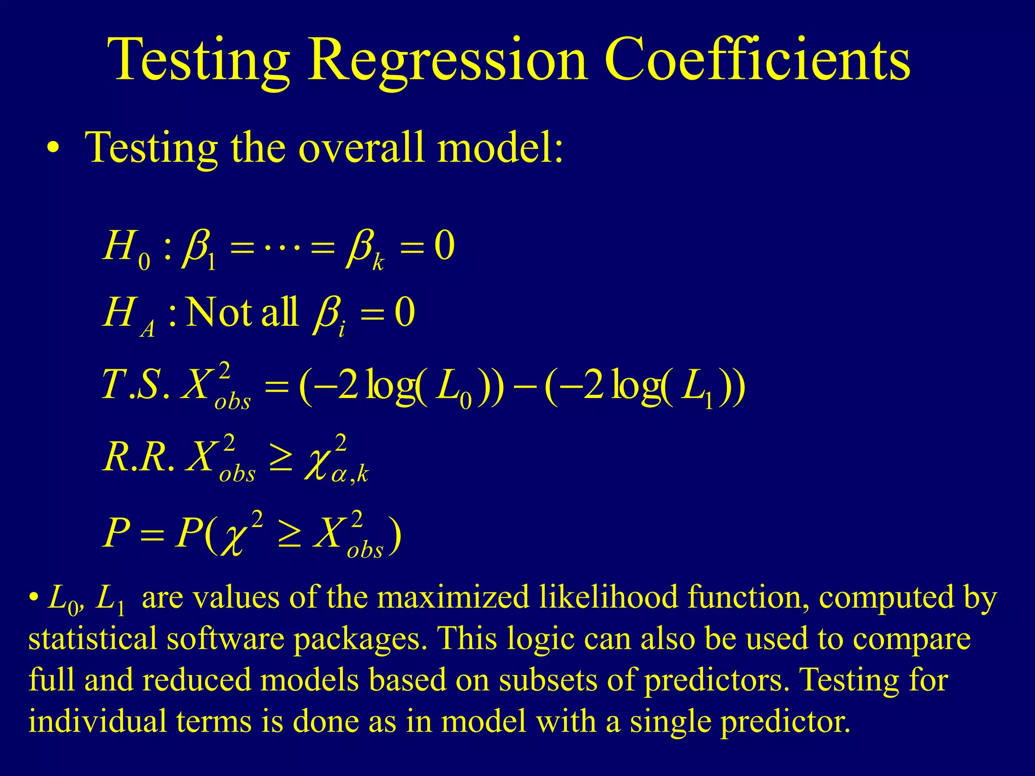
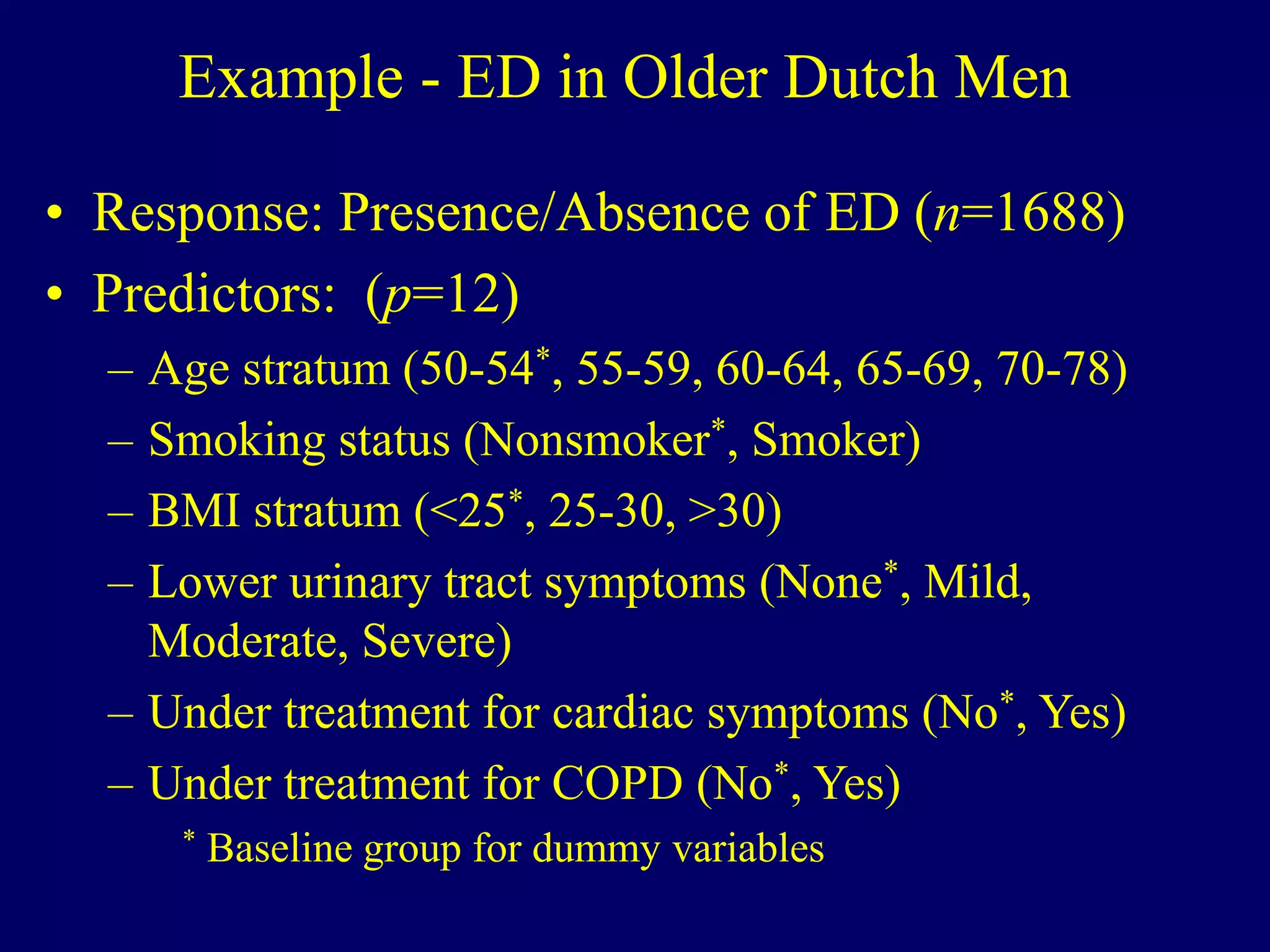
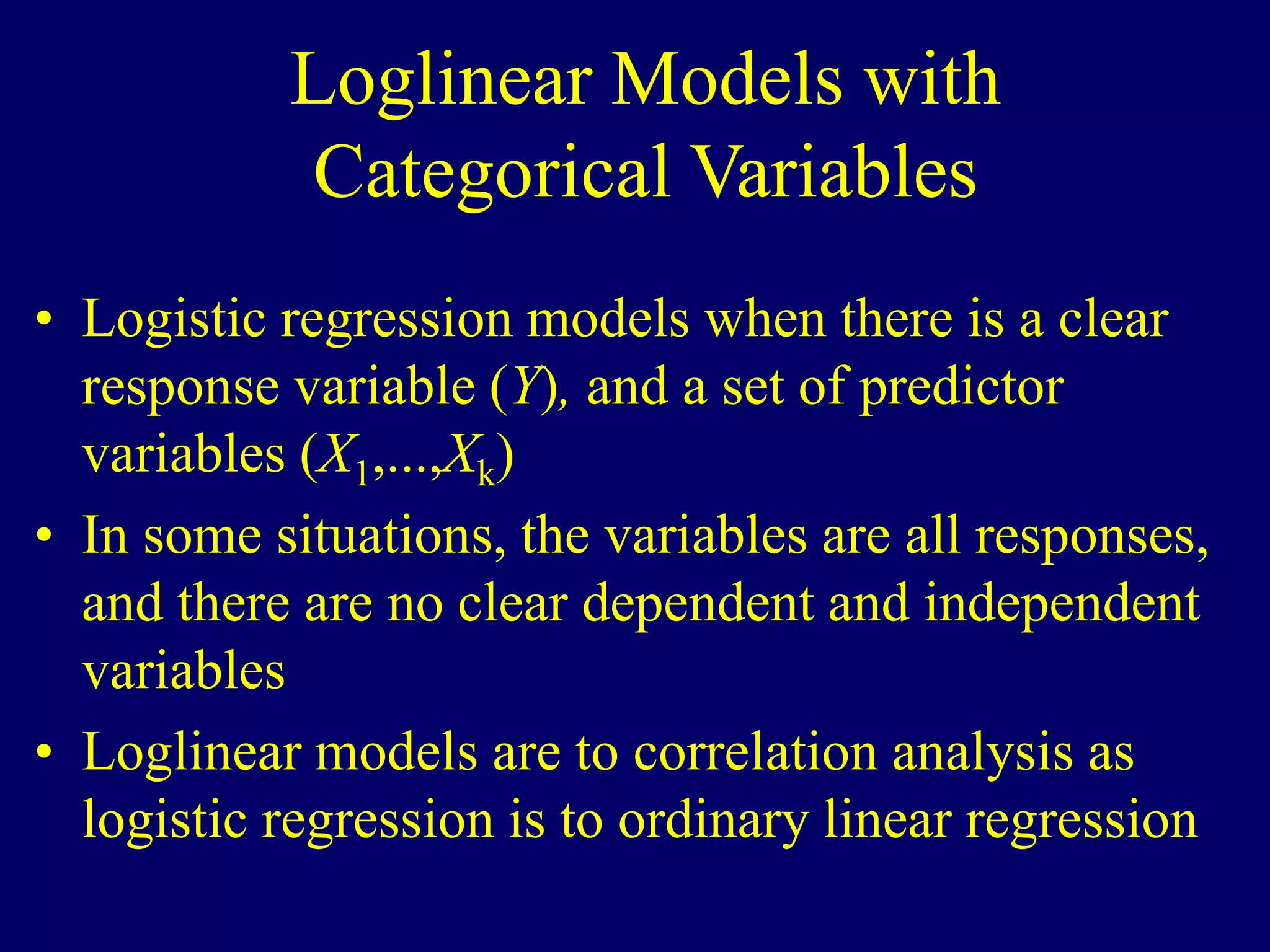
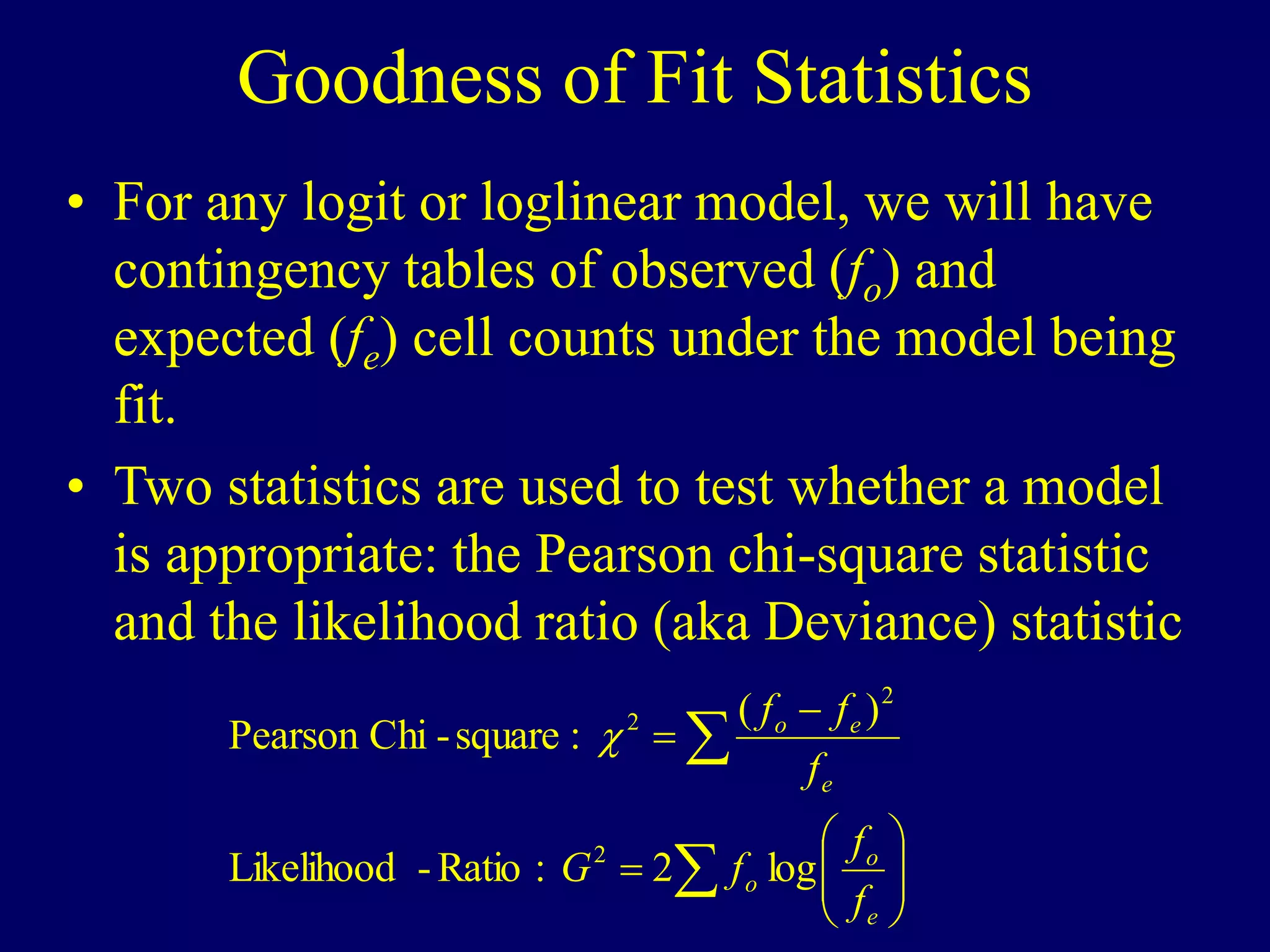
SlideShare a Scribd company logo
1 of 37
Logistic Regression
• Logistic Regression - Dichotomous Response
variable and numeric and/or categorical
explanatory variable(s)
– Goal: Model the probability of a particular as a function
of the predictor variable(s)
– Problem: Probabilities are bounded between 0 and 1
• Distribution of Responses: Binomial
• Link Function:













1
log
)
(
g
Logistic Regression with 1 Predictor
• Response - Presence/Absence of characteristic
• Predictor - Numeric variable observed for each case
• Model - p(x)  Probability of presence at predictor level x
x
x
e
e
x 



p 



1
)
(
•  = 0  P(Presence) is the same at each level of x
•  > 0  P(Presence) increases as x increases
•  < 0  P(Presence) decreases as x increases
Logistic Regression with 1 Predictor
 ,  are unknown parameters and must be
estimated using statistical software such as SPSS,
SAS, or STATA
· Primary interest in estimating and testing
hypotheses regarding 
· Large-Sample test (Wald Test):
· H0:  = 0 HA:   0
)
(
:
:
.
.
:
.
.
2
2
2
1
,
2
2
^
^
2
^
obs
obs
obs
X
P
val
P
X
R
R
X
S
T






















Example - Rizatriptan for Migraine
• Response - Complete Pain Relief at 2 hours (Yes/No)
• Predictor - Dose (mg): Placebo (0),2.5,5,10
Dose # Patients # Relieved % Relieved
0 67 2 3.0
2.5 75 7 9.3
5 130 29 22.3
10 145 40 27.6
Example - Rizatriptan for Migraine (SPSS)
t
5
7
9
1
0
0
0
5
6
1
0
3
D
C
S
1
a
B
. E
a
d
ig
p
V
a
x
x
e
e
x 165
.
0
490
.
2
165
.
0
490
.
2
^
1
)
( 





p
000
.
:
84
.
3
:
819
.
19
037
.
0
165
.
0
:
.
.
0
:
0
:
2
1
,
05
.
2
2
2
0
val
P
X
RR
X
S
T
H
H
obs
obs
A
















Odds Ratio
• Interpretation of Regression Coefficient ():
– In linear regression, the slope coefficient is the change
in the mean response as x increases by 1 unit
– In logistic regression, we can show that:












)
(
1
)
(
)
(
)
(
)
1
(
x
x
x
odds
e
x
odds
x
odds
p
p

• Thus e represents the change in the odds of the outcome
(multiplicatively) by increasing x by 1 unit
• If  = 0, the odds and probability are the same at all x levels (e=1)
• If  > 0 , the odds and probability increase as x increases (e>1)
• If  < 0 , the odds and probability decrease as x increases (e<1)
95% Confidence Interval for Odds Ratio
• Step 1: Construct a 95% CI for  :









 ^
^
^
^
^
^
^
^
^
96
.
1
,
96
.
1
96
.
1 

 





• Step 2: Raise e = 2.718 to the lower and upper bounds of the CI:





 

^
^
^
^
^
^
96
.
1
96
.
1
, 
 



e
e
• If entire interval is above 1, conclude positive association
• If entire interval is below 1, conclude negative association
• If interval contains 1, cannot conclude there is an association
Example - Rizatriptan for Migraine
)
2375
.
0
,
0925
.
0
(
)
037
.
0
(
96
.
1
165
.
0
:
%
95
037
.
0
165
.
0 ^
^
^




CI



• 95% CI for  :
• 95% CI for population odds ratio:
  )
27
.
1
,
10
.
1
(
, 2375
.
0
0925
.
0

e
e
• Conclude positive association between dose and
probability of complete relief
Multiple Logistic Regression
• Extension to more than one predictor variable (either
numeric or dummy variables).
• With k predictors, the model is written:
k
k
k
k
x
x
x
x
e
e






p 






 

1
1
1
1
1
• Adjusted Odds ratio for raising xi by 1 unit, holding
all other predictors constant:
i
e
ORi


• Many models have nominal/ordinal predictors, and
widely make use of dummy variables
Testing Regression Coefficients
• Testing the overall model:
)
(
.
.
))
log(
2
(
))
log(
2
(
.
.
0
all
Not
:
0
:
2
2
2
,
2
1
0
2
1
0
obs
k
obs
obs
i
A
k
X
P
P
X
R
R
L
L
X
S
T
H
H


















• L0, L1 are values of the maximized likelihood function, computed by
statistical software packages. This logic can also be used to compare
full and reduced models based on subsets of predictors. Testing for
individual terms is done as in model with a single predictor.
Example - ED in Older Dutch Men
• Response: Presence/Absence of ED (n=1688)
• Predictors: (p=12)
– Age stratum (50-54*, 55-59, 60-64, 65-69, 70-78)
– Smoking status (Nonsmoker*, Smoker)
– BMI stratum (<25*, 25-30, >30)
– Lower urinary tract symptoms (None*, Mild,
Moderate, Severe)
– Under treatment for cardiac symptoms (No*, Yes)
– Under treatment for COPD (No*, Yes)
* Baseline group for dummy variables
Example - ED in Older Dutch Men
Predictor b sb Adjusted OR (95% CI)
Age 55-59 (vs 50-54) 0.83 0.42 2.3 (1.0 – 5.2)
Age 60-64 (vs 50-54) 1.53 0.40 4.6 (2.1 – 10.1)
Age 65-69 (vs 50-54) 2.19 0.40 8.9 (4.1 – 19.5)
Age 70-78 (vs 50-54) 2.66 0.41 14.3 (6.4 – 32.1)
Smoker (vs nonsmoker) 0.47 0.19 1.6 (1.1 – 2.3)
BMI 25-30 (vs <25) 0.41 0.21 1.5 (1.0 – 2.3)
BMI >30 (vs <25) 1.10 0.29 3.0 (1.7 – 5.4)
LUTS Mild (vs None) 0.59 0.41 1.8 (0.8 – 4.3)
LUTS Moderate (vs None) 1.22 0.45 3.4 (1.4 – 8.4)
LUTS Severe (vs None) 2.01 0.56 7.5 (2.5 – 22.5)
Cardiac symptoms (Yes vs No) 0.92 0.26 2.5 (1.5 – 4.3)
COPD (Yes vs No) 0.64 0.28 1.9 (1.1 – 3.6)
Interpretations: Risk of ED appears to be:
• Increasing with age, BMI, and LUTS strata
• Higher among smokers
• Higher among men being treated for cardiac or COPD
Loglinear Models with
Categorical Variables
• Logistic regression models when there is a clear
response variable (Y), and a set of predictor
variables (X1,...,Xk)
• In some situations, the variables are all responses,
and there are no clear dependent and independent
variables
• Loglinear models are to correlation analysis as
logistic regression is to ordinary linear regression
Loglinear Models
• Example: 3 variables (X,Y,Z) each with 2 levels
• Can be set up in a 2x2x2 contingency table
• Hierarchy of Models:
– All variables are conditionally independent
– Two of the pairs of variables are conditionally
independent
– One of the pairs are conditionally independent
– No pairs are conditionally independent, but each
association is constant across levels of third variable
(no interaction or homogeneous association)
– All pairs are associated, and associations differ
among levels of third variable
Loglinear Models
• To determine associations, must have a measure: the
odds ratio (OR)
• Odds Ratios take on the value 1 if there is no
association
• Loglinear models make use of regressions with
coefficients being exponents. Thus, tests of whether
odds ratios are 1, is equivalently to testing whether
regression coefficients are 0 (as in logistic regression)
• For a given partial table, OR=e, software packages
estimate and test whether =0
Example - Feminine Traits/Behavior
3 Variables, each at 2 levels (Table contains observed counts):
Feminine Personality Trait (Modern/Traditional)
Female Role Behavior (Modern/Traditional)
Class (Lower Classman/Upper Classman)
*
C
3
5
8
1
3
4
4
8
2
9
3
2
0
5
5
9
8
7
M
T
P
T
M
T
P
T
C
L
U
d
i t
E B
o t
Example - Feminine Traits/Behavior
• Expected cell counts under model that allows for association
among all pairs of variables, but no interaction (association
between personality and role is same for each class, etc).
Model:(PR,PC,RC)
– Evidence of personality/role association (see odds ratios)
Class=Lower Class=Lower Class=Upper Class=Upper
Role=M Role=T Role=M Role=T
Personality=M 34.1 23.9 17.9 14.1
Personality=T 19.9 54.1 11.1 33.9
88
.
3
)
1
.
11
(
1
.
14
)
9
.
33
(
9
.
17
:
Upper
Class
88
.
3
)
9
.
19
(
9
.
23
)
1
.
54
(
1
.
34
:
Lower
Class






OR
OR
Note that under the no
interaction model, the odds
ratios measuring the
personality/role association
is same for each class
Example - Feminine Traits/Behavior
Role=M Role=M Role=T Role=T
Class=Lower Class=Upper Class=Lower Class=Upper
Personality=M 34.1 17.9 23.9 14.1
Personality=T 19.9 11.1 54.1 33.9
06
.
1
)
1
.
54
(
1
.
14
)
9
.
33
(
9
.
23
:
T
Role
06
.
1
)
9
.
19
(
9
.
17
)
1
.
11
(
1
.
34
:
M
Role






OR
OR
Personality=M Personality=M Personality=T Personality=T
Class=Lower Class=Upper Class=Lower Class=Upper
Role=M 34.1 17.9 19.9 11.1
Role=T 23.9 14.1 54.1 33.9
12
.
1
)
1
.
54
(
1
.
11
)
9
.
33
(
9
.
19
:
T
y
Personalit
12
.
1
)
9
.
23
(
9
.
17
)
1
.
14
(
1
.
34
:
M
y
Personalit






OR
OR
Example - Feminine Traits/Behavior
• Intuitive Results:
– Controlling for class in school, there is an
association between personality trait and role
behavior (ORLower=ORUpper=3.88)
– Controlling for role behavior there is no association
between personality trait and class (ORModern=
ORTraditional=1.06)
– Controlling for personality trait, there is no
association between role behavior and class
(ORModern= ORTraditional=1.12)
SPSS Output
• Statistical software packages fit regression type models, where
the regression coefficients for each model term are the log of the
odds ratio for that term, so that the estimated odds ratio is e
raised to the power of the regression coefficient.
Note: e1.3554 = 3.88 e.0605 = 1.06 e.1166 = 1.12
Parameter Estimates
Asymptotic 95% CI
Parameter Estimate SE Z-value Lower Upper
Constant 3.5234 .1651 21.35 3.20 3.85
Class .4674 .2050 2.28 .07 .87
Personality -.8774 .2726 -3.22 -1.41 -.34
Role -1.1166 .2873 -3.89 -1.68 -.55
C*P .0605 .3064 .20 -.54 .66
C*R .1166 .3107 .38 -.49 .73
R*P 1.3554 .2987 4.54 .77 1.94
Interpreting Coefficients
• The regression coefficients for each variable
corresponds to the lowest level (in alphanumeric
ordering of symbols). Computer output will print a
“mapping” of coefficients to variable levels.
Cell (C,P,R) Class  Prsnlty  Role  C*P  C*R  P*R  Expected Count
L,M,M 0.4674 -0.8774 -1.1166 0.0605 0.1166 1.3554 34.1
L,M,T 0.4674 -0.8774 0 0.0605 0 0 23.9
L,T,M 0.4674 0 -1.1166 0 0.1166 0 19.9
L,T,T 0.4674 0 0 0 0 0 54.1
U,M,M 0 -0.8774 -1.1166 0 0 1.3554 17.9
U,M,T 0 -0.8774 0 0 0 0 14.1
U,T,M 0 0 -1.1166 0 0 0 11.1
U,T,T 0 0 0 0 0 0 33.9
To obtain the expected cell counts, add the constant (3.5234) to
each of the s for that row, and raise e to the power of that sum
Goodness of Fit Statistics
• For any logit or loglinear model, we will have
contingency tables of observed (fo) and
expected (fe) cell counts under the model being
fit.
• Two statistics are used to test whether a model
is appropriate: the Pearson chi-square statistic
and the likelihood ratio (aka Deviance) statistic













e
o
o
e
e
o
f
f
f
G
f
f
f
log
2
:
Ratio
-
Likelihood
)
(
:
square
-
Chi
Pearson
2
2
2

Goodness of Fit Tests
• Null hypothesis: The current model is
appropriate
• Alternative hypothesis: Model is more complex
• Degrees of Freedom: Number of sample logits-
Number of parameters in model
• Distribution of Goodness of Fit statistics under
the null hypothesis is chi-square with degrees of
freedom given above
• Statistical software packages will print these
statistics and P-values.
Example - Feminine Traits/Behavior
Table Information
Observed Expected
Factor Value Count % Count %
PRSNALTY Modern
ROLEBHVR Modern
CLASS1 Lower Classman 33.00 ( 15.79) 34.10 ( 16.32)
CLASS1 Upper Classman 19.00 ( 9.09) 17.90 ( 8.57)
ROLEBHVR Traditional
CLASS1 Lower Classman 25.00 ( 11.96) 23.90 ( 11.44)
CLASS1 Upper Classman 13.00 ( 6.22) 14.10 ( 6.75)
PRSNALTY Traditional
ROLEBHVR Modern
CLASS1 Lower Classman 21.00 ( 10.05) 19.90 ( 9.52)
CLASS1 Upper Classman 10.00 ( 4.78) 11.10 ( 5.31)
ROLEBHVR Traditional
CLASS1 Lower Classman 53.00 ( 25.36) 54.10 ( 25.88)
CLASS1 Upper Classman 35.00 ( 16.75) 33.90 ( 16.22)
Goodness-of-fit Statistics
Chi-Square DF Sig.
Likelihood Ratio .4695 1 .4932
Pearson .4664 1 .4946
Example - Feminine Traits/Behavior
Goodness of fit statistics/tests for all possible models:
Model G2
2
df P-value (G2
) P-value (2
)
(C,P,R) 22.21 22.46 4 .0002 .0002
(C,PR) 0.7199 0.7232 3 .8685 .8677
(P,CR) 21.99 22.24 3 .00007 .00006
(R,CP) 22.04 22.34 3 .00006 .00006
(CR,CP) 22.93 22.13 2 .00002 .00002
(CP,PR) 0.6024 0.6106 2 .7399 .7369
(CR,PR) 0.5047 0.5085 2 .7770 .7755
(CP,CR,PR) 0.4644 0.4695 1 .4946 .4932
The simplest model for which we fail to reject the null
hypothesis that the model is adequate is: (C,PR): Personality
and Role are the only associated pair.
Adjusted Residuals
• Standardized differences between actual and
expected counts (fo-fe, divided by its
standard error).
• Large adjusted residuals (bigger than 3 in
absolute value, is a conservative rule of
thumb) are cells that show lack of fit of
current model
• Software packages will print these for logit
and loglinear models
Example - Feminine Traits/Behavior
• Adjusted residuals for (C,P,R) model of all
pairs being conditionally independent:
Adj.
Factor Value Resid. Resid.
PRSNALTY Modern
ROLEBHVR Modern
CLASS1 Lower Classman 10.43 3.04**
CLASS1 Upper Classman 5.83 1.99
ROLEBHVR Traditional
CLASS1 Lower Classman -9.27 -2.46
CLASS1 Upper Classman -6.99 -2.11
PRSNALTY Traditional
ROLEBHVR Modern
CLASS1 Lower Classman -8.85 -2.42
CLASS1 Upper Classman -7.41 -2.32
ROLEBHVR Traditional
CLASS1 Lower Classman 7.69 1.93
CLASS1 Upper Classman 8.57 2.41
Comparing Models with G2 Statistic
• Comparing a series of models that increase in
complexity.
• Take the difference in the deviance (G2) for the
models (less complex model minus more
complex model)
• Take the difference in degrees of freedom for the
models
• Under hypothesis that less complex (reduced)
model is adequate, difference follows chi-square
distribution
Example - Feminine Traits/Behavior
• Comparing a model where only Personality
and Role are associated (Reduced Model)
with the model where all pairs are associated
with no interaction (Full Model).
• Reduced Model (C,PR): G2=.7232, df=3
• Full Model (CP,CR,PR): G2=.4695, df=1
• Difference: .7232-.4695=.2537, df=3-1=2
• Critical value (=0.05): 5.99
• Conclude Reduced Model is adequate
Logit Models for Ordinal Responses
• Response variable is ordinal (categorical
with natural ordering)
• Predictor variable(s) can be numeric or
qualitative (dummy variables)
• Labeling the ordinal categories from 1
(lowest level) to c (highest), can obtain the
cumulative probabilities:
c
j
j
Y
P
Y
P
j
Y
P ,
,
1
)
(
)
1
(
)
( 
 






Logistic Regression for Ordinal Response
• The odds of falling in category j or below:
1
)
(
1
,
,
1
)
(
)
(






c
Y
P
c
j
j
Y
P
j
Y
P

• Logit (log odds) of cumulative probabilities are modeled
as linear functions of predictor variable(s):
  1
,
,
1
)
(
)
(
log
)
(
logit 












 c
j
X
j
Y
P
j
Y
P
j
Y
P j 


This is called the proportional odds model, and assumes the
effect of X is the same for each cumulative probability
Example - Urban Renewal Attitudes
• Response: Attitude toward urban renewal
project (Negative (Y=1), Moderate (Y=2),
Positive (Y=3))
• Predictor Variable: Respondent’s Race
(White, Nonwhite)
• Contingency Table:
AttitudeRace White Nonwhite
Negative (Y=1) 101 106
Moderate (Y=2) 91 127
Positive (Y=3) 170 190
SPSS Output
• Note that SPSS fits the model in the
following form:
  1
,
,
1
)
(
)
(
log
)
(
logit 












 c
j
X
j
Y
P
j
Y
P
j
Y
P j 


r E
7
2
3
1
0
7
8
5
4
0
1
0
0
1
1
3
0
1
3
3
0
0 a
.
.
0
.
.
.
[ A
[ A
T
[ R
[ R
L
m
E
a
d f
S i g
r B
r B
d e
L
T
a
Note that the race variable is not significant (or even close).
Fitted Equation
• The fitted equation for each group/category:
165
.
0
0
165
.
0
)
Nonwhite
|
2
(
)
Nonwhite
|
2
(
logit
:
te
Mod/Nonwhi
or
Neg
166
.
0
)
001
.
0
(
165
.
0
)
White
|
2
(
)
White
|
2
(
logit
:
Mod/White
or
Neg
027
.
1
)
0
(
027
.
1
)
Nonwhite
|
1
(
)
Nonwhite
|
1
(
logit
:
onwhite
Negative/N
026
.
1
)
001
.
0
(
027
.
1
)
White
|
1
(
)
White
|
1
(
logit
:
hite
Negative/W


















































Y
P
Y
P
Y
P
Y
P
Y
P
Y
P
Y
P
Y
P
For each group, the fitted probability of falling in that set of categories
is eL/(1+eL) where L is the logit value (0.264,0.264,0.541,0.541)
Inference for Regression Coefficients
• If  = 0, the response (Y) is independent of X
• Z-test can be conducted to test this (estimate
divided by its standard error)
• Most software will conduct the Wald test, with the
statistic being the z-statistic squared, which has a
chi-squared distribution with 1 degree of freedom
under the null hypothesis
• Odds ratio of increasing X by 1 unit and its
confidence interval are obtained by raising e to the
power of the regression coefficient and its upper
and lower bounds
Example - Urban Renewal Attitudes
• Z-statistic for testing for race differences:
Z=0.001/0.133 = 0.0075 (recall model estimates -)
• Wald statistic: .000 (P-value=.993)
• Estimated odds ratio: e.001 = 1.001
• 95% Confidence Interval: (e-.260,e.263)=(0.771,1.301)
• Interval contains 1, odds of being in a given category or
below is same for whites as nonwhites
r E
7
2
3
1
0
7
8
5
4
0
1
0
0
1
1
3
0
1
3
3
0
0 a
.
.
0
.
.
.
[ A
[ A
T
[ R
[ R
L
m
E
a
d f
S i g
r B
r B
d e
L
T
a
Ordinal Predictors
• Creating dummy variables for ordinal
categories treats them as if nominal
• To make an ordinal variable, create a new
variable X that models the levels of the
ordinal variable
• Setting depends on assignment of levels
(simplest form is to let X=1,...,c for the
categories which treats levels as being
equally spaced)

More Related Content

Similar to chapter15c.ppt

Chapter 9Multivariable MethodsObjectives• .docx
Chapter 9Multivariable MethodsObjectives• .docxChapter 9Multivariable MethodsObjectives• .docx
Chapter 9Multivariable MethodsObjectives• .docx
spoonerneddy
 

Similar to chapter15c.ppt (20)

Logistic regression vs. logistic classifier. History of the confusion and the...
Logistic regression vs. logistic classifier. History of the confusion and the...Logistic regression vs. logistic classifier. History of the confusion and the...
Logistic regression vs. logistic classifier. History of the confusion and the...
 
Biostatistics lecture notes 7.ppt
Biostatistics lecture notes 7.pptBiostatistics lecture notes 7.ppt
Biostatistics lecture notes 7.ppt
 
Dr.Dinesh-BIOSTAT-Tests-of-significance-1-min.pdf
Dr.Dinesh-BIOSTAT-Tests-of-significance-1-min.pdfDr.Dinesh-BIOSTAT-Tests-of-significance-1-min.pdf
Dr.Dinesh-BIOSTAT-Tests-of-significance-1-min.pdf
 
3010l8.pdf
3010l8.pdf3010l8.pdf
3010l8.pdf
 
Logistic regression with SPSS examples
Logistic regression with SPSS examplesLogistic regression with SPSS examples
Logistic regression with SPSS examples
 
Proportions and Confidence Intervals in Biostatistics
Proportions and Confidence Intervals in BiostatisticsProportions and Confidence Intervals in Biostatistics
Proportions and Confidence Intervals in Biostatistics
 
Module 2_ Regression Models..pptx
Module 2_ Regression Models..pptxModule 2_ Regression Models..pptx
Module 2_ Regression Models..pptx
 
Medical statistics2
Medical statistics2Medical statistics2
Medical statistics2
 
Lect w8 w9_correlation_regression
Lect w8 w9_correlation_regressionLect w8 w9_correlation_regression
Lect w8 w9_correlation_regression
 
univariate and bivariate analysis in spss
univariate and bivariate analysis in spss univariate and bivariate analysis in spss
univariate and bivariate analysis in spss
 
9618821.ppt
9618821.ppt9618821.ppt
9618821.ppt
 
9618821.pdf
9618821.pdf9618821.pdf
9618821.pdf
 
Test of significance
Test of significanceTest of significance
Test of significance
 
Chapter 9Multivariable MethodsObjectives• .docx
Chapter 9Multivariable MethodsObjectives• .docxChapter 9Multivariable MethodsObjectives• .docx
Chapter 9Multivariable MethodsObjectives• .docx
 
Lecture 4
Lecture 4Lecture 4
Lecture 4
 
Topic 1 part 2
Topic 1 part 2Topic 1 part 2
Topic 1 part 2
 
Stat2013
Stat2013Stat2013
Stat2013
 
Lecture 4
Lecture 4Lecture 4
Lecture 4
 
604_multiplee.ppt
604_multiplee.ppt604_multiplee.ppt
604_multiplee.ppt
 
Measures of dispersion discuss 2.2
Measures of dispersion discuss 2.2Measures of dispersion discuss 2.2
Measures of dispersion discuss 2.2
 

More from MohamedSahal16 (7)

DOC-20221212-WA0035..pptx
DOC-20221212-WA0035..pptxDOC-20221212-WA0035..pptx
DOC-20221212-WA0035..pptx
 
ASP.pptx
ASP.pptxASP.pptx
ASP.pptx
 
Tutorial15_Programming.pptx
Tutorial15_Programming.pptxTutorial15_Programming.pptx
Tutorial15_Programming.pptx
 
chapter1IntroductiontoStatistics.ppt
chapter1IntroductiontoStatistics.pptchapter1IntroductiontoStatistics.ppt
chapter1IntroductiontoStatistics.ppt
 
Tutorial1_EViews_Basics.pptx
Tutorial1_EViews_Basics.pptxTutorial1_EViews_Basics.pptx
Tutorial1_EViews_Basics.pptx
 
New Microsoft PowerPoint Presentation.pptx
New Microsoft PowerPoint Presentation.pptxNew Microsoft PowerPoint Presentation.pptx
New Microsoft PowerPoint Presentation.pptx
 
Chapter 14.pptx
Chapter 14.pptxChapter 14.pptx
Chapter 14.pptx
 

Recently uploaded

1:1原版定制伦敦政治经济学院毕业证(LSE毕业证)成绩单学位证书留信学历认证
1:1原版定制伦敦政治经济学院毕业证(LSE毕业证)成绩单学位证书留信学历认证1:1原版定制伦敦政治经济学院毕业证(LSE毕业证)成绩单学位证书留信学历认证
1:1原版定制伦敦政治经济学院毕业证(LSE毕业证)成绩单学位证书留信学历认证
dq9vz1isj
 
一比一原版麦考瑞大学毕业证成绩单如何办理
一比一原版麦考瑞大学毕业证成绩单如何办理一比一原版麦考瑞大学毕业证成绩单如何办理
一比一原版麦考瑞大学毕业证成绩单如何办理
cyebo
 
Audience Researchndfhcvnfgvgbhujhgfv.pptx
Audience Researchndfhcvnfgvgbhujhgfv.pptxAudience Researchndfhcvnfgvgbhujhgfv.pptx
Audience Researchndfhcvnfgvgbhujhgfv.pptx
Stephen266013
 
NO1 Best Kala Jadu Expert Specialist In Germany Kala Jadu Expert Specialist I...
NO1 Best Kala Jadu Expert Specialist In Germany Kala Jadu Expert Specialist I...NO1 Best Kala Jadu Expert Specialist In Germany Kala Jadu Expert Specialist I...
NO1 Best Kala Jadu Expert Specialist In Germany Kala Jadu Expert Specialist I...
Amil baba
 
Abortion pills in Riyadh Saudi Arabia (+966572737505 buy cytotec
Abortion pills in Riyadh Saudi Arabia (+966572737505 buy cytotecAbortion pills in Riyadh Saudi Arabia (+966572737505 buy cytotec
Abortion pills in Riyadh Saudi Arabia (+966572737505 buy cytotec
Abortion pills in Riyadh +966572737505 get cytotec
 
Data Analytics for Digital Marketing Lecture for Advanced Digital & Social Me...
Data Analytics for Digital Marketing Lecture for Advanced Digital & Social Me...Data Analytics for Digital Marketing Lecture for Advanced Digital & Social Me...
Data Analytics for Digital Marketing Lecture for Advanced Digital & Social Me...
Valters Lauzums
 
原件一样(UWO毕业证书)西安大略大学毕业证成绩单留信学历认证
原件一样(UWO毕业证书)西安大略大学毕业证成绩单留信学历认证原件一样(UWO毕业证书)西安大略大学毕业证成绩单留信学历认证
原件一样(UWO毕业证书)西安大略大学毕业证成绩单留信学历认证
pwgnohujw
 
如何办理英国卡迪夫大学毕业证(Cardiff毕业证书)成绩单留信学历认证
如何办理英国卡迪夫大学毕业证(Cardiff毕业证书)成绩单留信学历认证如何办理英国卡迪夫大学毕业证(Cardiff毕业证书)成绩单留信学历认证
如何办理英国卡迪夫大学毕业证(Cardiff毕业证书)成绩单留信学历认证
ju0dztxtn
 

Recently uploaded (20)

Atlantic Grupa Case Study (Mintec Data AI)
Atlantic Grupa Case Study (Mintec Data AI)Atlantic Grupa Case Study (Mintec Data AI)
Atlantic Grupa Case Study (Mintec Data AI)
 
Predictive Precipitation: Advanced Rain Forecasting Techniques
Predictive Precipitation: Advanced Rain Forecasting TechniquesPredictive Precipitation: Advanced Rain Forecasting Techniques
Predictive Precipitation: Advanced Rain Forecasting Techniques
 
Bios of leading Astrologers & Researchers
Bios of leading Astrologers & ResearchersBios of leading Astrologers & Researchers
Bios of leading Astrologers & Researchers
 
社内勉強会資料  Mamba - A new era or ephemeral
社内勉強会資料   Mamba - A new era or ephemeral社内勉強会資料   Mamba - A new era or ephemeral
社内勉強会資料  Mamba - A new era or ephemeral
 
1:1原版定制伦敦政治经济学院毕业证(LSE毕业证)成绩单学位证书留信学历认证
1:1原版定制伦敦政治经济学院毕业证(LSE毕业证)成绩单学位证书留信学历认证1:1原版定制伦敦政治经济学院毕业证(LSE毕业证)成绩单学位证书留信学历认证
1:1原版定制伦敦政治经济学院毕业证(LSE毕业证)成绩单学位证书留信学历认证
 
Identify Rules that Predict Patient’s Heart Disease - An Application of Decis...
Identify Rules that Predict Patient’s Heart Disease - An Application of Decis...Identify Rules that Predict Patient’s Heart Disease - An Application of Decis...
Identify Rules that Predict Patient’s Heart Disease - An Application of Decis...
 
一比一原版麦考瑞大学毕业证成绩单如何办理
一比一原版麦考瑞大学毕业证成绩单如何办理一比一原版麦考瑞大学毕业证成绩单如何办理
一比一原版麦考瑞大学毕业证成绩单如何办理
 
Audience Researchndfhcvnfgvgbhujhgfv.pptx
Audience Researchndfhcvnfgvgbhujhgfv.pptxAudience Researchndfhcvnfgvgbhujhgfv.pptx
Audience Researchndfhcvnfgvgbhujhgfv.pptx
 
123.docx. .
123.docx.                                 .123.docx.                                 .
123.docx. .
 
NO1 Best Kala Jadu Expert Specialist In Germany Kala Jadu Expert Specialist I...
NO1 Best Kala Jadu Expert Specialist In Germany Kala Jadu Expert Specialist I...NO1 Best Kala Jadu Expert Specialist In Germany Kala Jadu Expert Specialist I...
NO1 Best Kala Jadu Expert Specialist In Germany Kala Jadu Expert Specialist I...
 
Aggregations - The Elasticsearch "GROUP BY"
Aggregations - The Elasticsearch "GROUP BY"Aggregations - The Elasticsearch "GROUP BY"
Aggregations - The Elasticsearch "GROUP BY"
 
How to Transform Clinical Trial Management with Advanced Data Analytics
How to Transform Clinical Trial Management with Advanced Data AnalyticsHow to Transform Clinical Trial Management with Advanced Data Analytics
How to Transform Clinical Trial Management with Advanced Data Analytics
 
Data Visualization Exploring and Explaining with Data 1st Edition by Camm sol...
Data Visualization Exploring and Explaining with Data 1st Edition by Camm sol...Data Visualization Exploring and Explaining with Data 1st Edition by Camm sol...
Data Visualization Exploring and Explaining with Data 1st Edition by Camm sol...
 
MATERI MANAJEMEN OF PENYAKIT TETANUS.ppt
MATERI  MANAJEMEN OF PENYAKIT TETANUS.pptMATERI  MANAJEMEN OF PENYAKIT TETANUS.ppt
MATERI MANAJEMEN OF PENYAKIT TETANUS.ppt
 
Abortion pills in Riyadh Saudi Arabia (+966572737505 buy cytotec
Abortion pills in Riyadh Saudi Arabia (+966572737505 buy cytotecAbortion pills in Riyadh Saudi Arabia (+966572737505 buy cytotec
Abortion pills in Riyadh Saudi Arabia (+966572737505 buy cytotec
 
Data Analytics for Digital Marketing Lecture for Advanced Digital & Social Me...
Data Analytics for Digital Marketing Lecture for Advanced Digital & Social Me...Data Analytics for Digital Marketing Lecture for Advanced Digital & Social Me...
Data Analytics for Digital Marketing Lecture for Advanced Digital & Social Me...
 
原件一样(UWO毕业证书)西安大略大学毕业证成绩单留信学历认证
原件一样(UWO毕业证书)西安大略大学毕业证成绩单留信学历认证原件一样(UWO毕业证书)西安大略大学毕业证成绩单留信学历认证
原件一样(UWO毕业证书)西安大略大学毕业证成绩单留信学历认证
 
Formulas dax para power bI de microsoft.pdf
Formulas dax para power bI de microsoft.pdfFormulas dax para power bI de microsoft.pdf
Formulas dax para power bI de microsoft.pdf
 
NOAM AAUG Adobe Summit 2024: Summit Slam Dunks
NOAM AAUG Adobe Summit 2024: Summit Slam DunksNOAM AAUG Adobe Summit 2024: Summit Slam Dunks
NOAM AAUG Adobe Summit 2024: Summit Slam Dunks
 
如何办理英国卡迪夫大学毕业证(Cardiff毕业证书)成绩单留信学历认证
如何办理英国卡迪夫大学毕业证(Cardiff毕业证书)成绩单留信学历认证如何办理英国卡迪夫大学毕业证(Cardiff毕业证书)成绩单留信学历认证
如何办理英国卡迪夫大学毕业证(Cardiff毕业证书)成绩单留信学历认证
 

chapter15c.ppt

  • 1. Logistic Regression • Logistic Regression - Dichotomous Response variable and numeric and/or categorical explanatory variable(s) – Goal: Model the probability of a particular as a function of the predictor variable(s) – Problem: Probabilities are bounded between 0 and 1 • Distribution of Responses: Binomial • Link Function:              1 log ) ( g
  • 2. Logistic Regression with 1 Predictor • Response - Presence/Absence of characteristic • Predictor - Numeric variable observed for each case • Model - p(x)  Probability of presence at predictor level x x x e e x     p     1 ) ( •  = 0  P(Presence) is the same at each level of x •  > 0  P(Presence) increases as x increases •  < 0  P(Presence) decreases as x increases
  • 3. Logistic Regression with 1 Predictor  ,  are unknown parameters and must be estimated using statistical software such as SPSS, SAS, or STATA · Primary interest in estimating and testing hypotheses regarding  · Large-Sample test (Wald Test): · H0:  = 0 HA:   0 ) ( : : . . : . . 2 2 2 1 , 2 2 ^ ^ 2 ^ obs obs obs X P val P X R R X S T                      
  • 4. Example - Rizatriptan for Migraine • Response - Complete Pain Relief at 2 hours (Yes/No) • Predictor - Dose (mg): Placebo (0),2.5,5,10 Dose # Patients # Relieved % Relieved 0 67 2 3.0 2.5 75 7 9.3 5 130 29 22.3 10 145 40 27.6
  • 5. Example - Rizatriptan for Migraine (SPSS) t 5 7 9 1 0 0 0 5 6 1 0 3 D C S 1 a B . E a d ig p V a x x e e x 165 . 0 490 . 2 165 . 0 490 . 2 ^ 1 ) (       p 000 . : 84 . 3 : 819 . 19 037 . 0 165 . 0 : . . 0 : 0 : 2 1 , 05 . 2 2 2 0 val P X RR X S T H H obs obs A                
  • 6. Odds Ratio • Interpretation of Regression Coefficient (): – In linear regression, the slope coefficient is the change in the mean response as x increases by 1 unit – In logistic regression, we can show that:             ) ( 1 ) ( ) ( ) ( ) 1 ( x x x odds e x odds x odds p p  • Thus e represents the change in the odds of the outcome (multiplicatively) by increasing x by 1 unit • If  = 0, the odds and probability are the same at all x levels (e=1) • If  > 0 , the odds and probability increase as x increases (e>1) • If  < 0 , the odds and probability decrease as x increases (e<1)
  • 7. 95% Confidence Interval for Odds Ratio • Step 1: Construct a 95% CI for  :           ^ ^ ^ ^ ^ ^ ^ ^ ^ 96 . 1 , 96 . 1 96 . 1          • Step 2: Raise e = 2.718 to the lower and upper bounds of the CI:         ^ ^ ^ ^ ^ ^ 96 . 1 96 . 1 ,       e e • If entire interval is above 1, conclude positive association • If entire interval is below 1, conclude negative association • If interval contains 1, cannot conclude there is an association
  • 8. Example - Rizatriptan for Migraine ) 2375 . 0 , 0925 . 0 ( ) 037 . 0 ( 96 . 1 165 . 0 : % 95 037 . 0 165 . 0 ^ ^ ^     CI    • 95% CI for  : • 95% CI for population odds ratio:   ) 27 . 1 , 10 . 1 ( , 2375 . 0 0925 . 0  e e • Conclude positive association between dose and probability of complete relief
  • 9. Multiple Logistic Regression • Extension to more than one predictor variable (either numeric or dummy variables). • With k predictors, the model is written: k k k k x x x x e e       p           1 1 1 1 1 • Adjusted Odds ratio for raising xi by 1 unit, holding all other predictors constant: i e ORi   • Many models have nominal/ordinal predictors, and widely make use of dummy variables
  • 10. Testing Regression Coefficients • Testing the overall model: ) ( . . )) log( 2 ( )) log( 2 ( . . 0 all Not : 0 : 2 2 2 , 2 1 0 2 1 0 obs k obs obs i A k X P P X R R L L X S T H H                   • L0, L1 are values of the maximized likelihood function, computed by statistical software packages. This logic can also be used to compare full and reduced models based on subsets of predictors. Testing for individual terms is done as in model with a single predictor.
  • 11. Example - ED in Older Dutch Men • Response: Presence/Absence of ED (n=1688) • Predictors: (p=12) – Age stratum (50-54*, 55-59, 60-64, 65-69, 70-78) – Smoking status (Nonsmoker*, Smoker) – BMI stratum (<25*, 25-30, >30) – Lower urinary tract symptoms (None*, Mild, Moderate, Severe) – Under treatment for cardiac symptoms (No*, Yes) – Under treatment for COPD (No*, Yes) * Baseline group for dummy variables
  • 12. Example - ED in Older Dutch Men Predictor b sb Adjusted OR (95% CI) Age 55-59 (vs 50-54) 0.83 0.42 2.3 (1.0 – 5.2) Age 60-64 (vs 50-54) 1.53 0.40 4.6 (2.1 – 10.1) Age 65-69 (vs 50-54) 2.19 0.40 8.9 (4.1 – 19.5) Age 70-78 (vs 50-54) 2.66 0.41 14.3 (6.4 – 32.1) Smoker (vs nonsmoker) 0.47 0.19 1.6 (1.1 – 2.3) BMI 25-30 (vs <25) 0.41 0.21 1.5 (1.0 – 2.3) BMI >30 (vs <25) 1.10 0.29 3.0 (1.7 – 5.4) LUTS Mild (vs None) 0.59 0.41 1.8 (0.8 – 4.3) LUTS Moderate (vs None) 1.22 0.45 3.4 (1.4 – 8.4) LUTS Severe (vs None) 2.01 0.56 7.5 (2.5 – 22.5) Cardiac symptoms (Yes vs No) 0.92 0.26 2.5 (1.5 – 4.3) COPD (Yes vs No) 0.64 0.28 1.9 (1.1 – 3.6) Interpretations: Risk of ED appears to be: • Increasing with age, BMI, and LUTS strata • Higher among smokers • Higher among men being treated for cardiac or COPD
  • 13. Loglinear Models with Categorical Variables • Logistic regression models when there is a clear response variable (Y), and a set of predictor variables (X1,...,Xk) • In some situations, the variables are all responses, and there are no clear dependent and independent variables • Loglinear models are to correlation analysis as logistic regression is to ordinary linear regression
  • 14. Loglinear Models • Example: 3 variables (X,Y,Z) each with 2 levels • Can be set up in a 2x2x2 contingency table • Hierarchy of Models: – All variables are conditionally independent – Two of the pairs of variables are conditionally independent – One of the pairs are conditionally independent – No pairs are conditionally independent, but each association is constant across levels of third variable (no interaction or homogeneous association) – All pairs are associated, and associations differ among levels of third variable
  • 15. Loglinear Models • To determine associations, must have a measure: the odds ratio (OR) • Odds Ratios take on the value 1 if there is no association • Loglinear models make use of regressions with coefficients being exponents. Thus, tests of whether odds ratios are 1, is equivalently to testing whether regression coefficients are 0 (as in logistic regression) • For a given partial table, OR=e, software packages estimate and test whether =0
  • 16. Example - Feminine Traits/Behavior 3 Variables, each at 2 levels (Table contains observed counts): Feminine Personality Trait (Modern/Traditional) Female Role Behavior (Modern/Traditional) Class (Lower Classman/Upper Classman) * C 3 5 8 1 3 4 4 8 2 9 3 2 0 5 5 9 8 7 M T P T M T P T C L U d i t E B o t
  • 17. Example - Feminine Traits/Behavior • Expected cell counts under model that allows for association among all pairs of variables, but no interaction (association between personality and role is same for each class, etc). Model:(PR,PC,RC) – Evidence of personality/role association (see odds ratios) Class=Lower Class=Lower Class=Upper Class=Upper Role=M Role=T Role=M Role=T Personality=M 34.1 23.9 17.9 14.1 Personality=T 19.9 54.1 11.1 33.9 88 . 3 ) 1 . 11 ( 1 . 14 ) 9 . 33 ( 9 . 17 : Upper Class 88 . 3 ) 9 . 19 ( 9 . 23 ) 1 . 54 ( 1 . 34 : Lower Class       OR OR Note that under the no interaction model, the odds ratios measuring the personality/role association is same for each class
  • 18. Example - Feminine Traits/Behavior Role=M Role=M Role=T Role=T Class=Lower Class=Upper Class=Lower Class=Upper Personality=M 34.1 17.9 23.9 14.1 Personality=T 19.9 11.1 54.1 33.9 06 . 1 ) 1 . 54 ( 1 . 14 ) 9 . 33 ( 9 . 23 : T Role 06 . 1 ) 9 . 19 ( 9 . 17 ) 1 . 11 ( 1 . 34 : M Role       OR OR Personality=M Personality=M Personality=T Personality=T Class=Lower Class=Upper Class=Lower Class=Upper Role=M 34.1 17.9 19.9 11.1 Role=T 23.9 14.1 54.1 33.9 12 . 1 ) 1 . 54 ( 1 . 11 ) 9 . 33 ( 9 . 19 : T y Personalit 12 . 1 ) 9 . 23 ( 9 . 17 ) 1 . 14 ( 1 . 34 : M y Personalit       OR OR
  • 19. Example - Feminine Traits/Behavior • Intuitive Results: – Controlling for class in school, there is an association between personality trait and role behavior (ORLower=ORUpper=3.88) – Controlling for role behavior there is no association between personality trait and class (ORModern= ORTraditional=1.06) – Controlling for personality trait, there is no association between role behavior and class (ORModern= ORTraditional=1.12)
  • 20. SPSS Output • Statistical software packages fit regression type models, where the regression coefficients for each model term are the log of the odds ratio for that term, so that the estimated odds ratio is e raised to the power of the regression coefficient. Note: e1.3554 = 3.88 e.0605 = 1.06 e.1166 = 1.12 Parameter Estimates Asymptotic 95% CI Parameter Estimate SE Z-value Lower Upper Constant 3.5234 .1651 21.35 3.20 3.85 Class .4674 .2050 2.28 .07 .87 Personality -.8774 .2726 -3.22 -1.41 -.34 Role -1.1166 .2873 -3.89 -1.68 -.55 C*P .0605 .3064 .20 -.54 .66 C*R .1166 .3107 .38 -.49 .73 R*P 1.3554 .2987 4.54 .77 1.94
  • 21. Interpreting Coefficients • The regression coefficients for each variable corresponds to the lowest level (in alphanumeric ordering of symbols). Computer output will print a “mapping” of coefficients to variable levels. Cell (C,P,R) Class  Prsnlty  Role  C*P  C*R  P*R  Expected Count L,M,M 0.4674 -0.8774 -1.1166 0.0605 0.1166 1.3554 34.1 L,M,T 0.4674 -0.8774 0 0.0605 0 0 23.9 L,T,M 0.4674 0 -1.1166 0 0.1166 0 19.9 L,T,T 0.4674 0 0 0 0 0 54.1 U,M,M 0 -0.8774 -1.1166 0 0 1.3554 17.9 U,M,T 0 -0.8774 0 0 0 0 14.1 U,T,M 0 0 -1.1166 0 0 0 11.1 U,T,T 0 0 0 0 0 0 33.9 To obtain the expected cell counts, add the constant (3.5234) to each of the s for that row, and raise e to the power of that sum
  • 22. Goodness of Fit Statistics • For any logit or loglinear model, we will have contingency tables of observed (fo) and expected (fe) cell counts under the model being fit. • Two statistics are used to test whether a model is appropriate: the Pearson chi-square statistic and the likelihood ratio (aka Deviance) statistic              e o o e e o f f f G f f f log 2 : Ratio - Likelihood ) ( : square - Chi Pearson 2 2 2 
  • 23. Goodness of Fit Tests • Null hypothesis: The current model is appropriate • Alternative hypothesis: Model is more complex • Degrees of Freedom: Number of sample logits- Number of parameters in model • Distribution of Goodness of Fit statistics under the null hypothesis is chi-square with degrees of freedom given above • Statistical software packages will print these statistics and P-values.
  • 24. Example - Feminine Traits/Behavior Table Information Observed Expected Factor Value Count % Count % PRSNALTY Modern ROLEBHVR Modern CLASS1 Lower Classman 33.00 ( 15.79) 34.10 ( 16.32) CLASS1 Upper Classman 19.00 ( 9.09) 17.90 ( 8.57) ROLEBHVR Traditional CLASS1 Lower Classman 25.00 ( 11.96) 23.90 ( 11.44) CLASS1 Upper Classman 13.00 ( 6.22) 14.10 ( 6.75) PRSNALTY Traditional ROLEBHVR Modern CLASS1 Lower Classman 21.00 ( 10.05) 19.90 ( 9.52) CLASS1 Upper Classman 10.00 ( 4.78) 11.10 ( 5.31) ROLEBHVR Traditional CLASS1 Lower Classman 53.00 ( 25.36) 54.10 ( 25.88) CLASS1 Upper Classman 35.00 ( 16.75) 33.90 ( 16.22) Goodness-of-fit Statistics Chi-Square DF Sig. Likelihood Ratio .4695 1 .4932 Pearson .4664 1 .4946
  • 25. Example - Feminine Traits/Behavior Goodness of fit statistics/tests for all possible models: Model G2 2 df P-value (G2 ) P-value (2 ) (C,P,R) 22.21 22.46 4 .0002 .0002 (C,PR) 0.7199 0.7232 3 .8685 .8677 (P,CR) 21.99 22.24 3 .00007 .00006 (R,CP) 22.04 22.34 3 .00006 .00006 (CR,CP) 22.93 22.13 2 .00002 .00002 (CP,PR) 0.6024 0.6106 2 .7399 .7369 (CR,PR) 0.5047 0.5085 2 .7770 .7755 (CP,CR,PR) 0.4644 0.4695 1 .4946 .4932 The simplest model for which we fail to reject the null hypothesis that the model is adequate is: (C,PR): Personality and Role are the only associated pair.
  • 26. Adjusted Residuals • Standardized differences between actual and expected counts (fo-fe, divided by its standard error). • Large adjusted residuals (bigger than 3 in absolute value, is a conservative rule of thumb) are cells that show lack of fit of current model • Software packages will print these for logit and loglinear models
  • 27. Example - Feminine Traits/Behavior • Adjusted residuals for (C,P,R) model of all pairs being conditionally independent: Adj. Factor Value Resid. Resid. PRSNALTY Modern ROLEBHVR Modern CLASS1 Lower Classman 10.43 3.04** CLASS1 Upper Classman 5.83 1.99 ROLEBHVR Traditional CLASS1 Lower Classman -9.27 -2.46 CLASS1 Upper Classman -6.99 -2.11 PRSNALTY Traditional ROLEBHVR Modern CLASS1 Lower Classman -8.85 -2.42 CLASS1 Upper Classman -7.41 -2.32 ROLEBHVR Traditional CLASS1 Lower Classman 7.69 1.93 CLASS1 Upper Classman 8.57 2.41
  • 28. Comparing Models with G2 Statistic • Comparing a series of models that increase in complexity. • Take the difference in the deviance (G2) for the models (less complex model minus more complex model) • Take the difference in degrees of freedom for the models • Under hypothesis that less complex (reduced) model is adequate, difference follows chi-square distribution
  • 29. Example - Feminine Traits/Behavior • Comparing a model where only Personality and Role are associated (Reduced Model) with the model where all pairs are associated with no interaction (Full Model). • Reduced Model (C,PR): G2=.7232, df=3 • Full Model (CP,CR,PR): G2=.4695, df=1 • Difference: .7232-.4695=.2537, df=3-1=2 • Critical value (=0.05): 5.99 • Conclude Reduced Model is adequate
  • 30. Logit Models for Ordinal Responses • Response variable is ordinal (categorical with natural ordering) • Predictor variable(s) can be numeric or qualitative (dummy variables) • Labeling the ordinal categories from 1 (lowest level) to c (highest), can obtain the cumulative probabilities: c j j Y P Y P j Y P , , 1 ) ( ) 1 ( ) (         
  • 31. Logistic Regression for Ordinal Response • The odds of falling in category j or below: 1 ) ( 1 , , 1 ) ( ) (       c Y P c j j Y P j Y P  • Logit (log odds) of cumulative probabilities are modeled as linear functions of predictor variable(s):   1 , , 1 ) ( ) ( log ) ( logit               c j X j Y P j Y P j Y P j    This is called the proportional odds model, and assumes the effect of X is the same for each cumulative probability
  • 32. Example - Urban Renewal Attitudes • Response: Attitude toward urban renewal project (Negative (Y=1), Moderate (Y=2), Positive (Y=3)) • Predictor Variable: Respondent’s Race (White, Nonwhite) • Contingency Table: AttitudeRace White Nonwhite Negative (Y=1) 101 106 Moderate (Y=2) 91 127 Positive (Y=3) 170 190
  • 33. SPSS Output • Note that SPSS fits the model in the following form:   1 , , 1 ) ( ) ( log ) ( logit               c j X j Y P j Y P j Y P j    r E 7 2 3 1 0 7 8 5 4 0 1 0 0 1 1 3 0 1 3 3 0 0 a . . 0 . . . [ A [ A T [ R [ R L m E a d f S i g r B r B d e L T a Note that the race variable is not significant (or even close).
  • 34. Fitted Equation • The fitted equation for each group/category: 165 . 0 0 165 . 0 ) Nonwhite | 2 ( ) Nonwhite | 2 ( logit : te Mod/Nonwhi or Neg 166 . 0 ) 001 . 0 ( 165 . 0 ) White | 2 ( ) White | 2 ( logit : Mod/White or Neg 027 . 1 ) 0 ( 027 . 1 ) Nonwhite | 1 ( ) Nonwhite | 1 ( logit : onwhite Negative/N 026 . 1 ) 001 . 0 ( 027 . 1 ) White | 1 ( ) White | 1 ( logit : hite Negative/W                                                   Y P Y P Y P Y P Y P Y P Y P Y P For each group, the fitted probability of falling in that set of categories is eL/(1+eL) where L is the logit value (0.264,0.264,0.541,0.541)
  • 35. Inference for Regression Coefficients • If  = 0, the response (Y) is independent of X • Z-test can be conducted to test this (estimate divided by its standard error) • Most software will conduct the Wald test, with the statistic being the z-statistic squared, which has a chi-squared distribution with 1 degree of freedom under the null hypothesis • Odds ratio of increasing X by 1 unit and its confidence interval are obtained by raising e to the power of the regression coefficient and its upper and lower bounds
  • 36. Example - Urban Renewal Attitudes • Z-statistic for testing for race differences: Z=0.001/0.133 = 0.0075 (recall model estimates -) • Wald statistic: .000 (P-value=.993) • Estimated odds ratio: e.001 = 1.001 • 95% Confidence Interval: (e-.260,e.263)=(0.771,1.301) • Interval contains 1, odds of being in a given category or below is same for whites as nonwhites r E 7 2 3 1 0 7 8 5 4 0 1 0 0 1 1 3 0 1 3 3 0 0 a . . 0 . . . [ A [ A T [ R [ R L m E a d f S i g r B r B d e L T a
  • 37. Ordinal Predictors • Creating dummy variables for ordinal categories treats them as if nominal • To make an ordinal variable, create a new variable X that models the levels of the ordinal variable • Setting depends on assignment of levels (simplest form is to let X=1,...,c for the categories which treats levels as being equally spaced)