Biostatistics

1. BASIC Biostatistics
Haramaya University
Collage of Health and Medicine Sciences
School of Public Health
LOGISTIC REGRESSION
February, 2025

2. Statistical model for Categorical data
The methods used in analysis of categorical variables
are:
Chi-squared Test
Logistic Regression

3. Chi-square test (x2
)
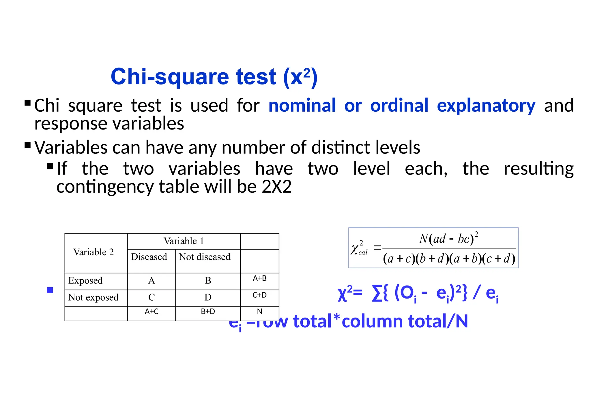
Chi square test is used for nominal or ordinal explanatory and
response variables
Variables can have any number of distinct levels
If the two variables have two level each, the resulting
contingency table will be 2X2
 χ2
= ∑{ (Oi - ei)2
} / ei
ei =row total*column total/N
Variable 2
Variable 1
Diseased Not diseased
Exposed A B A+B
Not exposed C D C+D
A+C B+D N
)
)(
)(
)(
(
)
(
d
c
b
a
d
b
c
a
bc
ad
N
cal






2
2


4. Chi-square test (x2
)
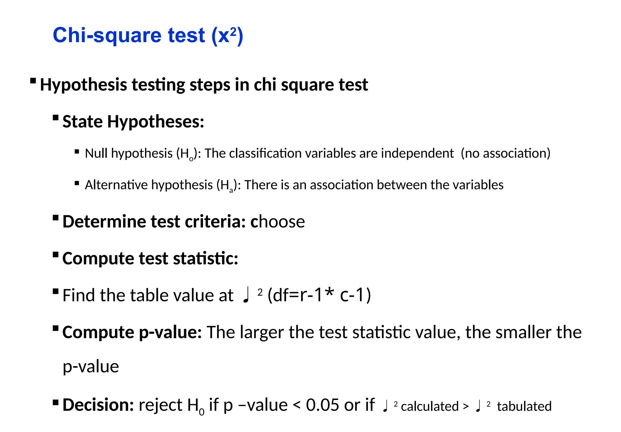
Hypothesis testing steps in chi square test
State Hypotheses:
 Null hypothesis (Ho): The classification variables are independent (no association)
 Alternative hypothesis (Ha): There is an association between the variables
Determine test criteria: choose
Compute test statistic:
Find the table value at 2
(df=r-1* c-1)
Compute p-value: The larger the test statistic value, the smaller the
p-value
Decision: reject H0 if p –value < 0.05 or if 2
calculated > 2
tabulated

5. Chi-square test (x2
)…
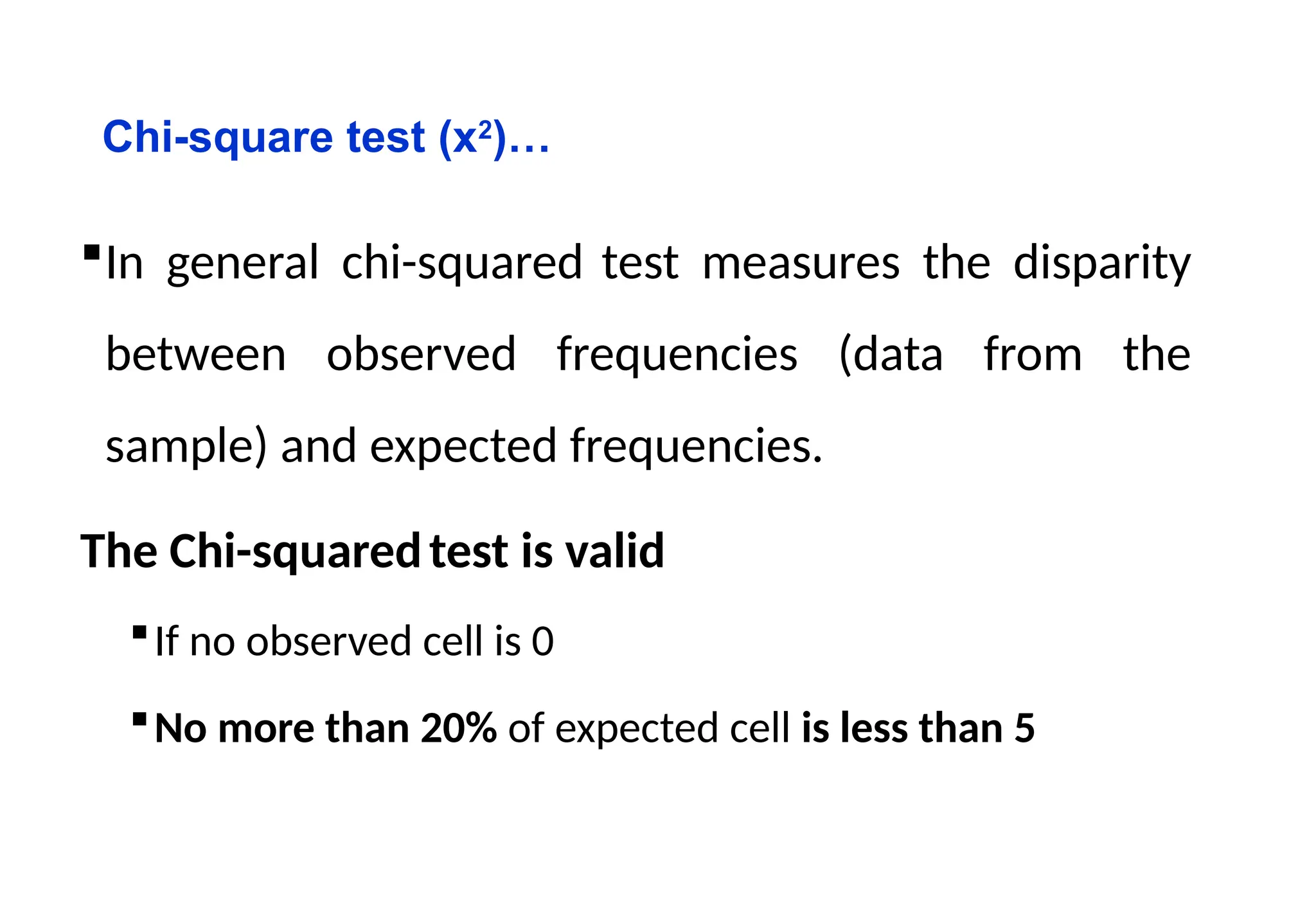
In general chi-squared test measures the disparity
between observed frequencies (data from the
sample) and expected frequencies.
The Chi-squaredtest is valid
If no observed cell is 0
No more than 20% of expected cell is less than 5

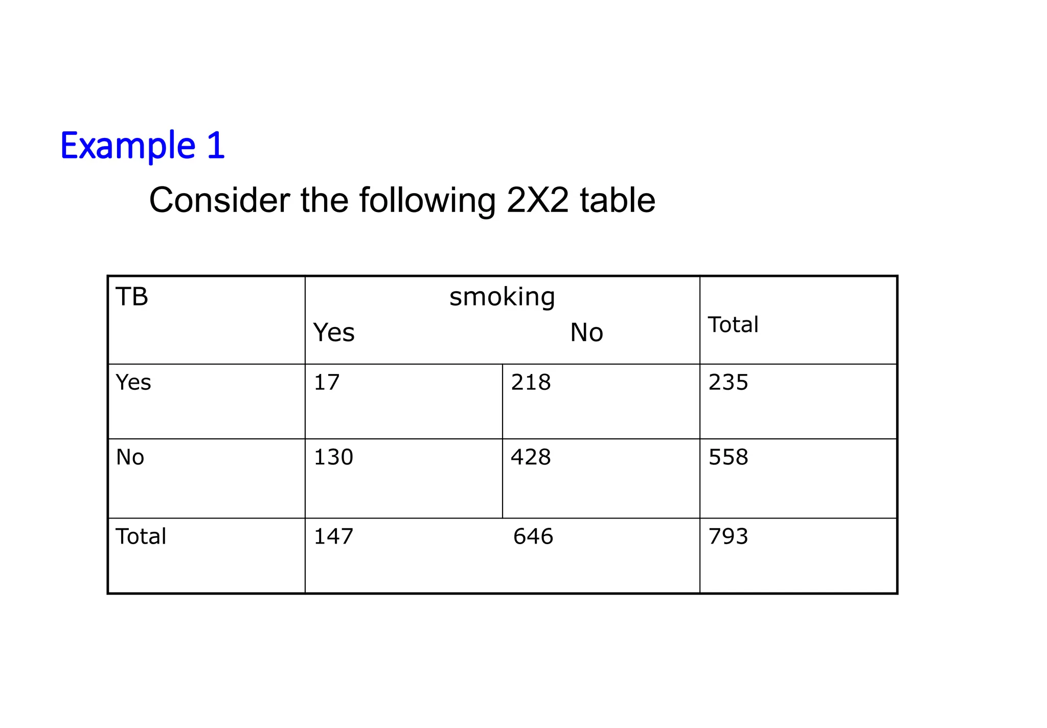
6. Example 1
TB smoking
Yes No Total
Yes 17 218 235
No 130 428 558
Total 147 646 793
Consider the following 2X2 table

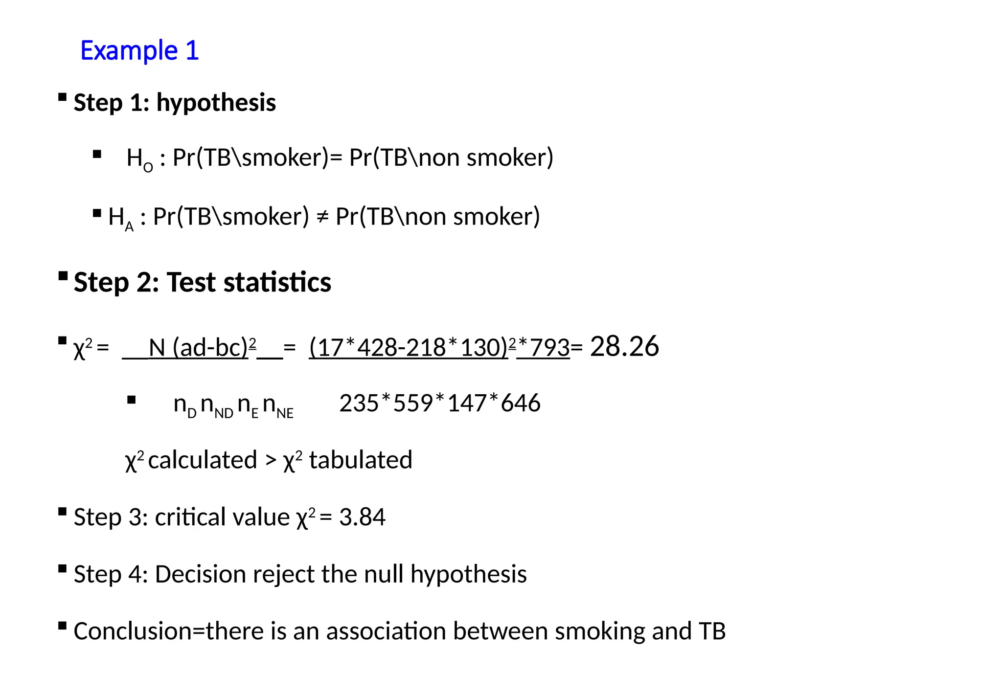
7. Example 1
 Step 1: hypothesis
 HO : Pr(TBsmoker)= Pr(TBnon smoker)
 HA : Pr(TBsmoker) ≠ Pr(TBnon smoker)
Step 2: Test statistics
 χ2
= __N (ad-bc)2
__= (17*428-218*130)2
*793= 28.26
 nD nND nE nNE 235*559*147*646
χ2
calculated > χ2
tabulated
 Step 3: critical value χ2
= 3.84
 Step 4: Decision reject the null hypothesis
 Conclusion=there is an association between smoking and TB

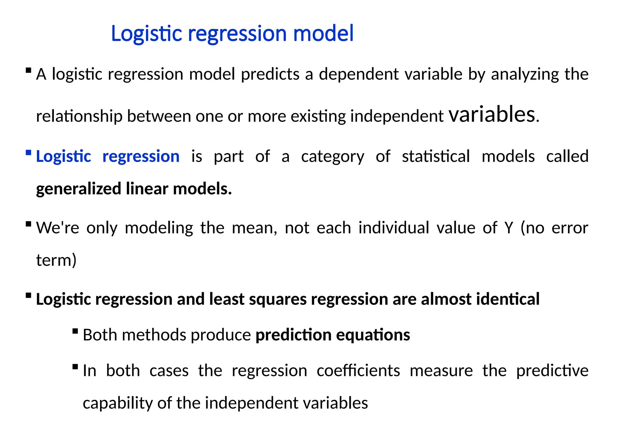
8. Logistic regression model
 A logistic regression model predicts a dependent variable by analyzing the
relationship between one or more existing independent variables.
 Logistic regression is part of a category of statistical models called
generalized linear models.
 We're only modeling the mean, not each individual value of Y (no error
term)
 Logistic regression and least squares regression are almost identical
 Both methods produce prediction equations
 In both cases the regression coefficients measure the predictive
capability of the independent variables

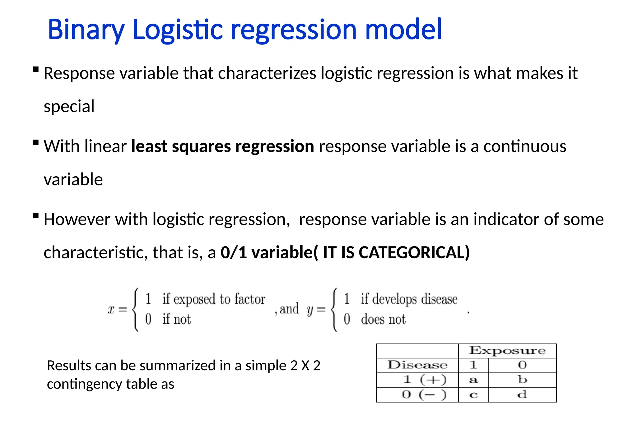
9. Binary Logistic regression model
 Response variable that characterizes logistic regression is what makes it
special
 With linear least squares regression response variable is a continuous
variable
 However with logistic regression, response variable is an indicator of some
characteristic, that is, a 0/1 variable( IT IS CATEGORICAL)
Results can be summarized in a simple 2 X 2
contingency table as

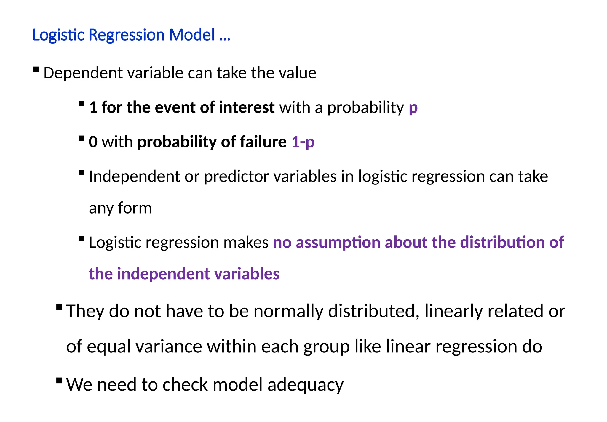
10. Logistic Regression Model …
 Dependent variable can take the value
 1 for the event of interest with a probability p
 0 with probability of failure 1-p
 Independent or predictor variables in logistic regression can take
any form
 Logistic regression makes no assumption about the distribution of
the independent variables
They do not have to be normally distributed, linearly related or
of equal variance within each group like linear regression do
We need to check model adequacy

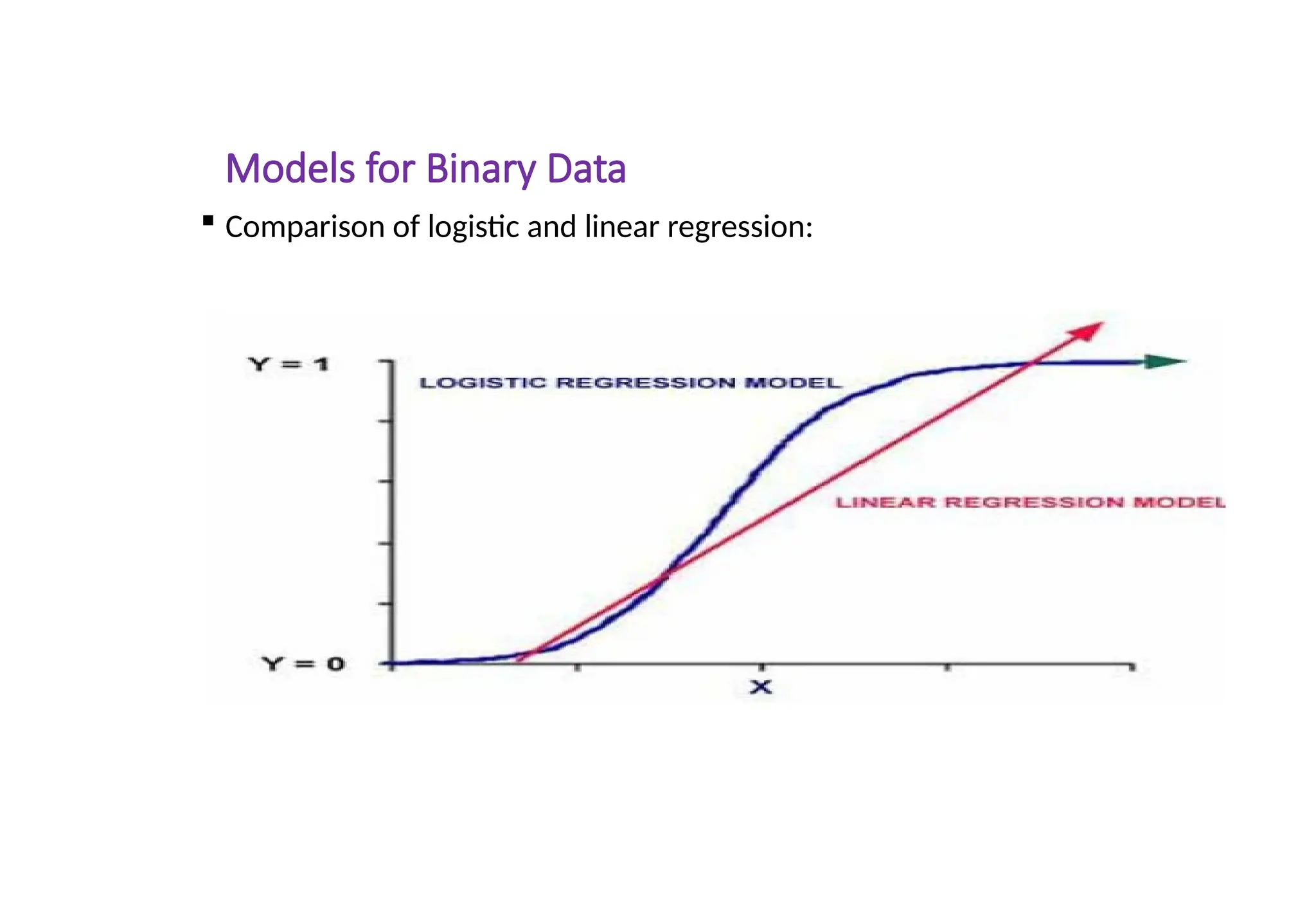
11. Models for Binary Data
 Comparison of logistic and linear regression:

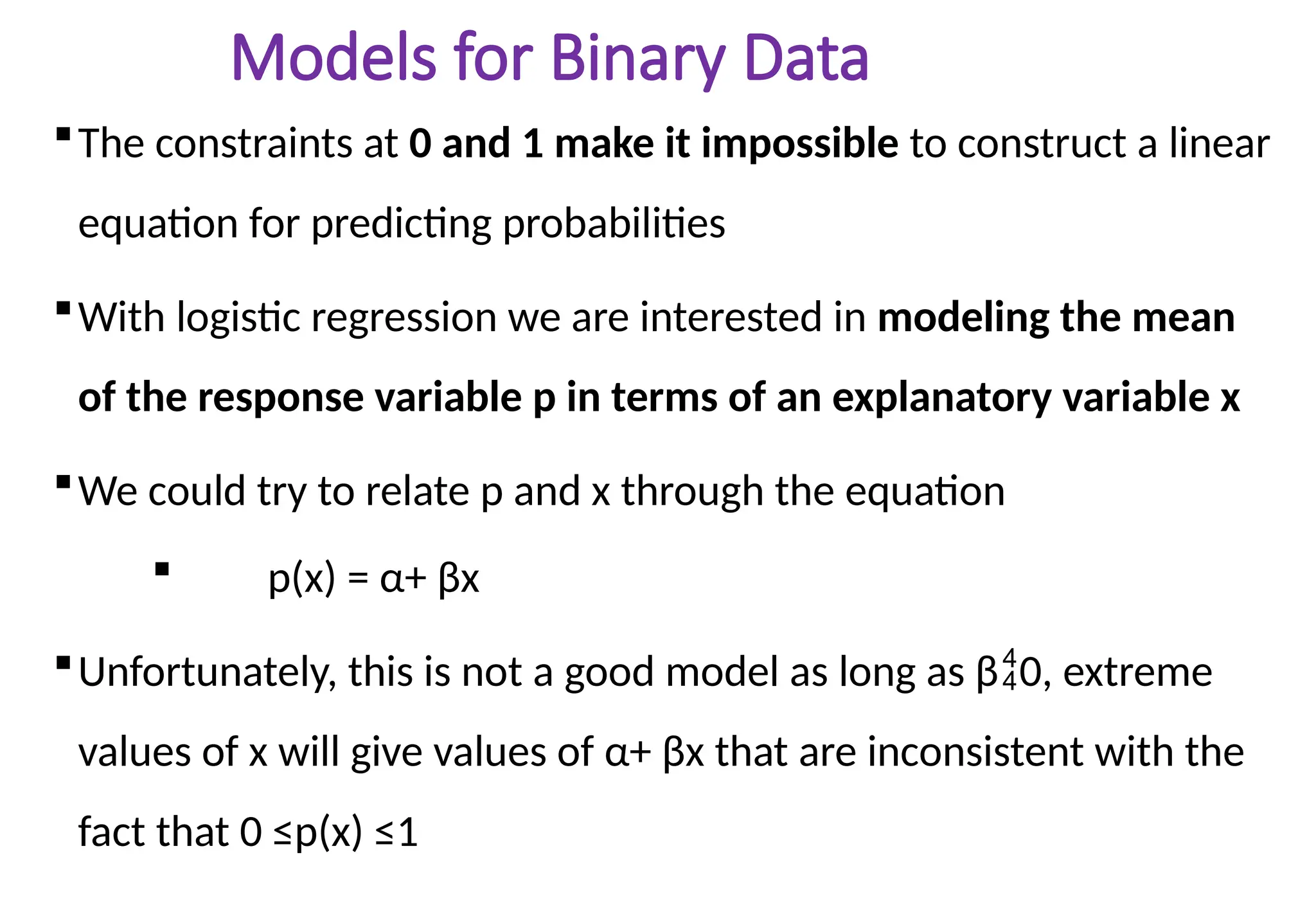
12. Models for Binary Data
The constraints at 0 and 1 make it impossible to construct a linear
equation for predicting probabilities
With logistic regression we are interested in modeling the mean
of the response variable p in terms of an explanatory variable x
We could try to relate p and x through the equation
 p(x) = α+ βx
Unfortunately, this is not a good model as long as β0, extreme
values of x will give values of α+ βx that are inconsistent with the
fact that 0 ≤p(x) ≤1

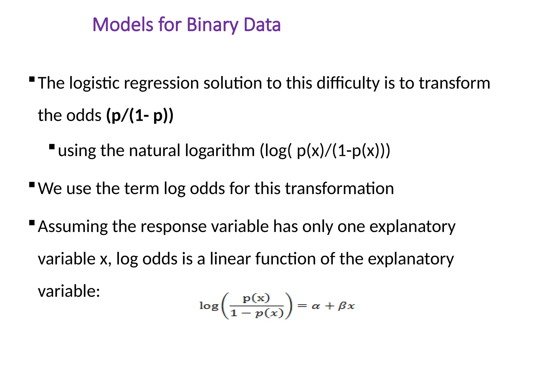
13. Models for Binary Data
The logistic regression solution to this difficulty is to transform
the odds (p/(1- p))
using the natural logarithm (log( p(x)/(1-p(x)))
We use the term log odds for this transformation
Assuming the response variable has only one explanatory
variable x, log odds is a linear function of the explanatory
variable:

14. Models for Binary Data
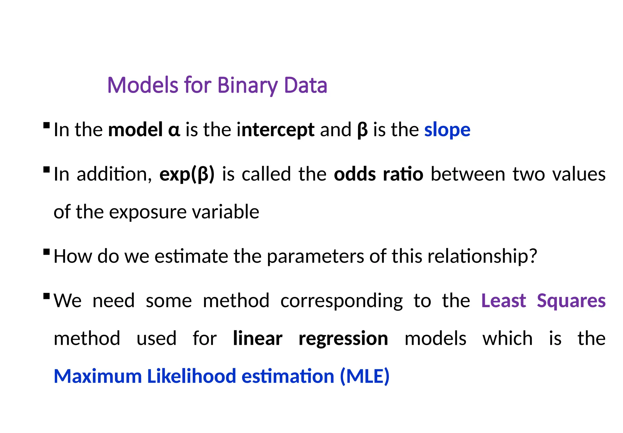
In the model α is the intercept and β is the slope
In addition, exp(β) is called the odds ratio between two values
of the exposure variable
How do we estimate the parameters of this relationship?
We need some method corresponding to the Least Squares
method used for linear regression models which is the
Maximum Likelihood estimation (MLE)

15. Likelihood Function and Maximum Likelihood Estimation
Maximum likelihood estimate of a parameter is the parameter
value for which the probability of the observed data takes its
greatest value
 It is the parameter value at which the likelihood function takes
its maximum

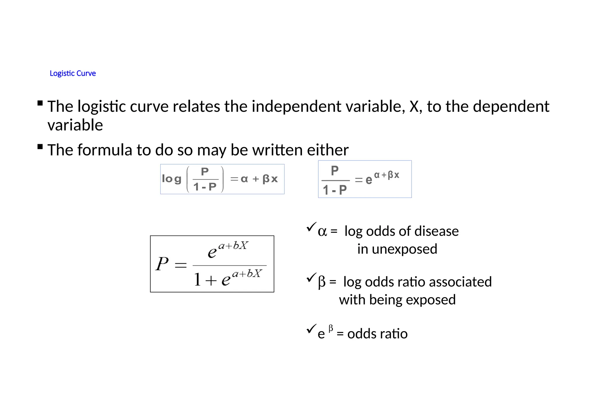
16. Logistic Curve
 The logistic curve relates the independent variable, X, to the dependent
variable
 The formula to do so may be written either
a = log odds of disease
in unexposed
b = log odds ratio associated
with being exposed
e
b
= odds ratio
βx
α
P
-
1
P
log 







e
P
-
1
P βx
α 


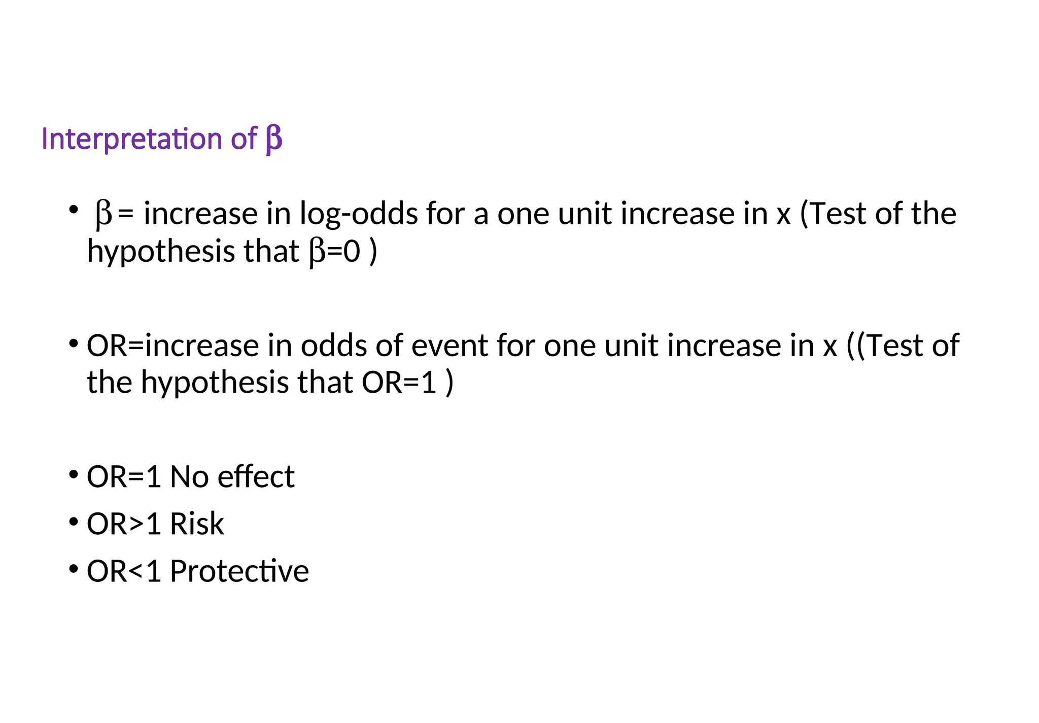
17. Interpretation of b
• b= increase in log-odds for a one unit increase in x (Test of the
hypothesis that b=0 )
• OR=increase in odds of event for one unit increase in x ((Test of
the hypothesis that OR=1 )
• OR=1 No effect
• OR>1 Risk
• OR<1 Protective

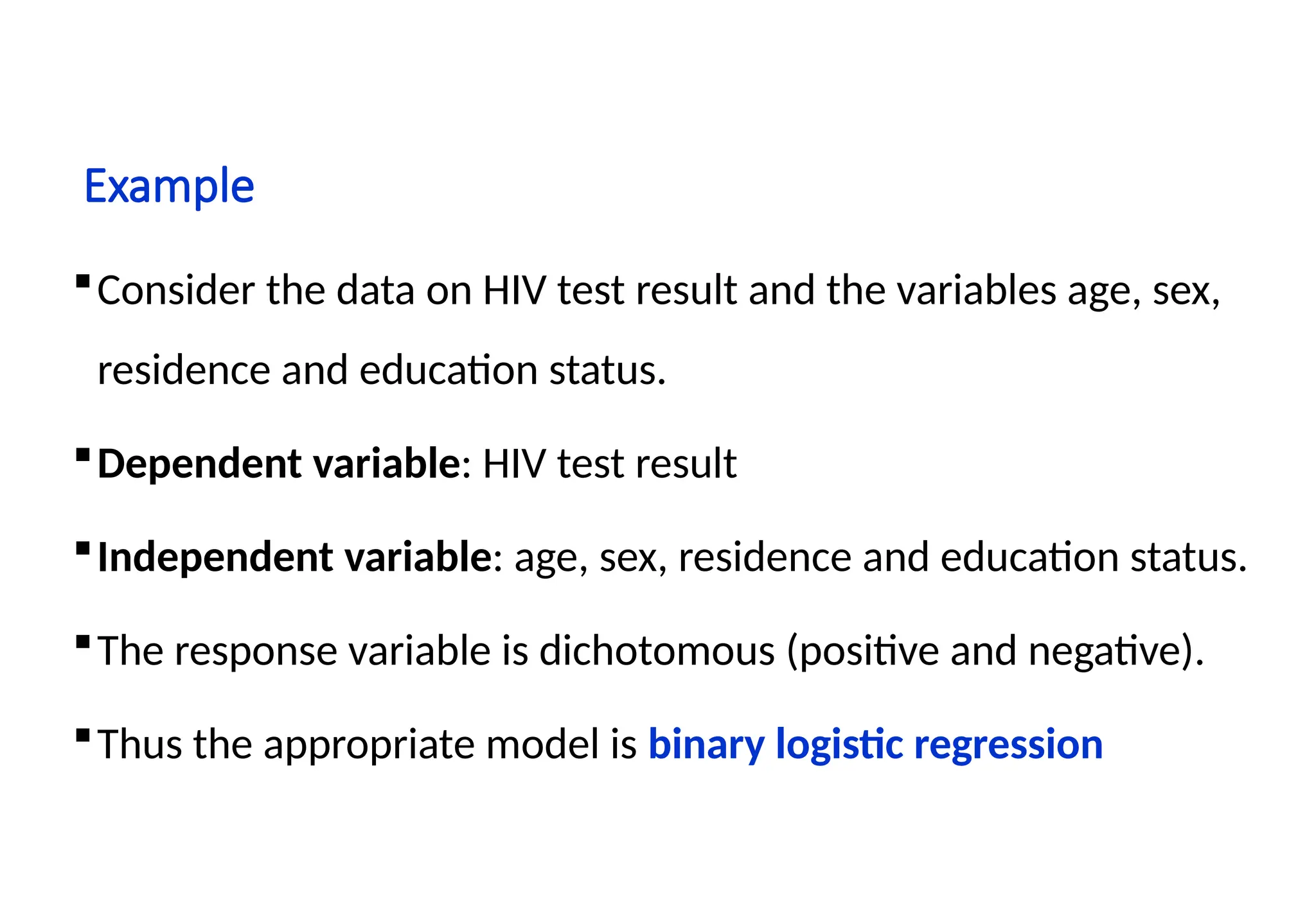
18. Example
Consider the data on HIV test result and the variables age, sex,
residence and education status.
Dependent variable: HIV test result
Independent variable: age, sex, residence and education status.
The response variable is dichotomous (positive and negative).
Thus the appropriate model is binary logistic regression

19. SPSS Application
• Analyze  Regression  binary logistic

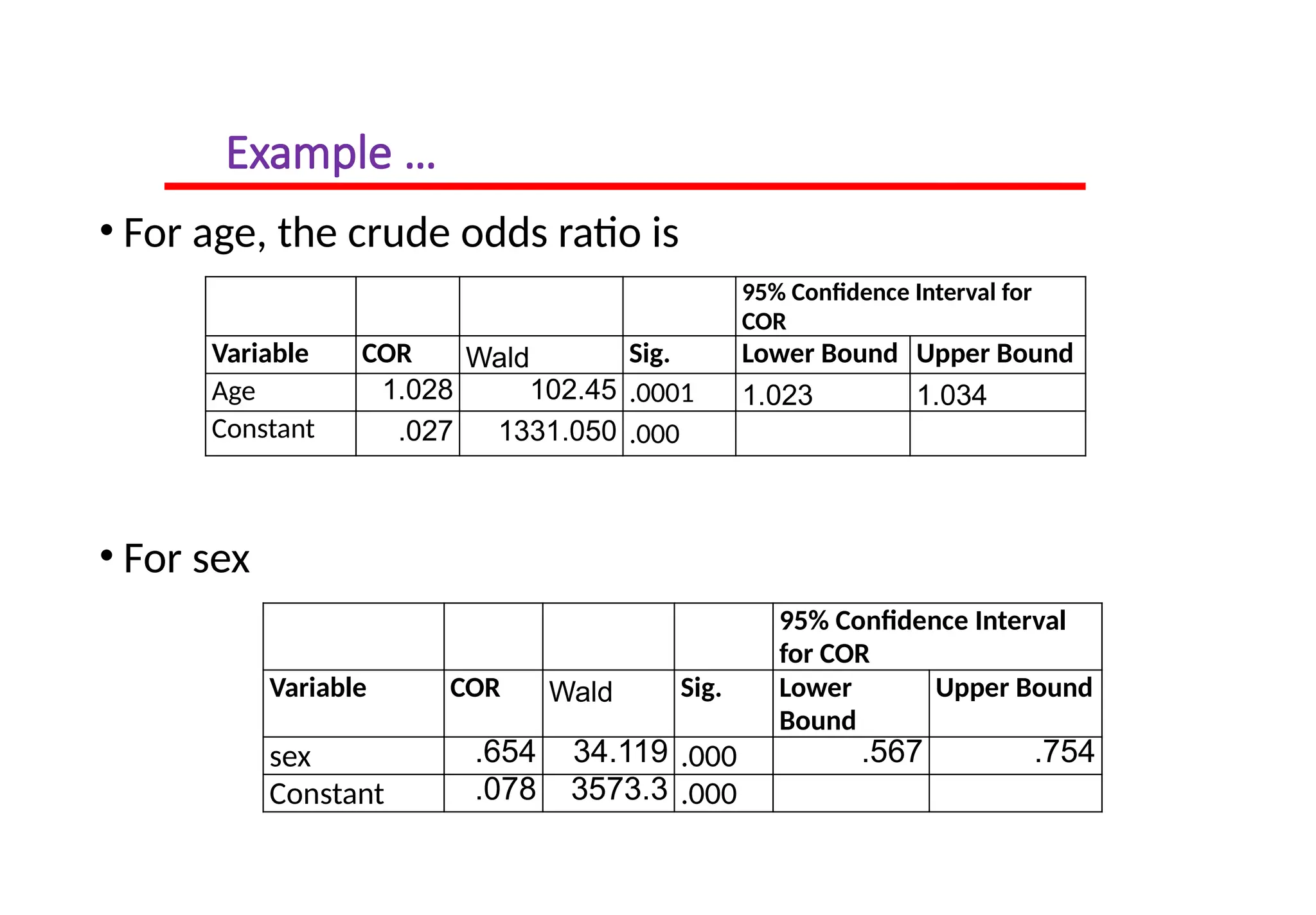
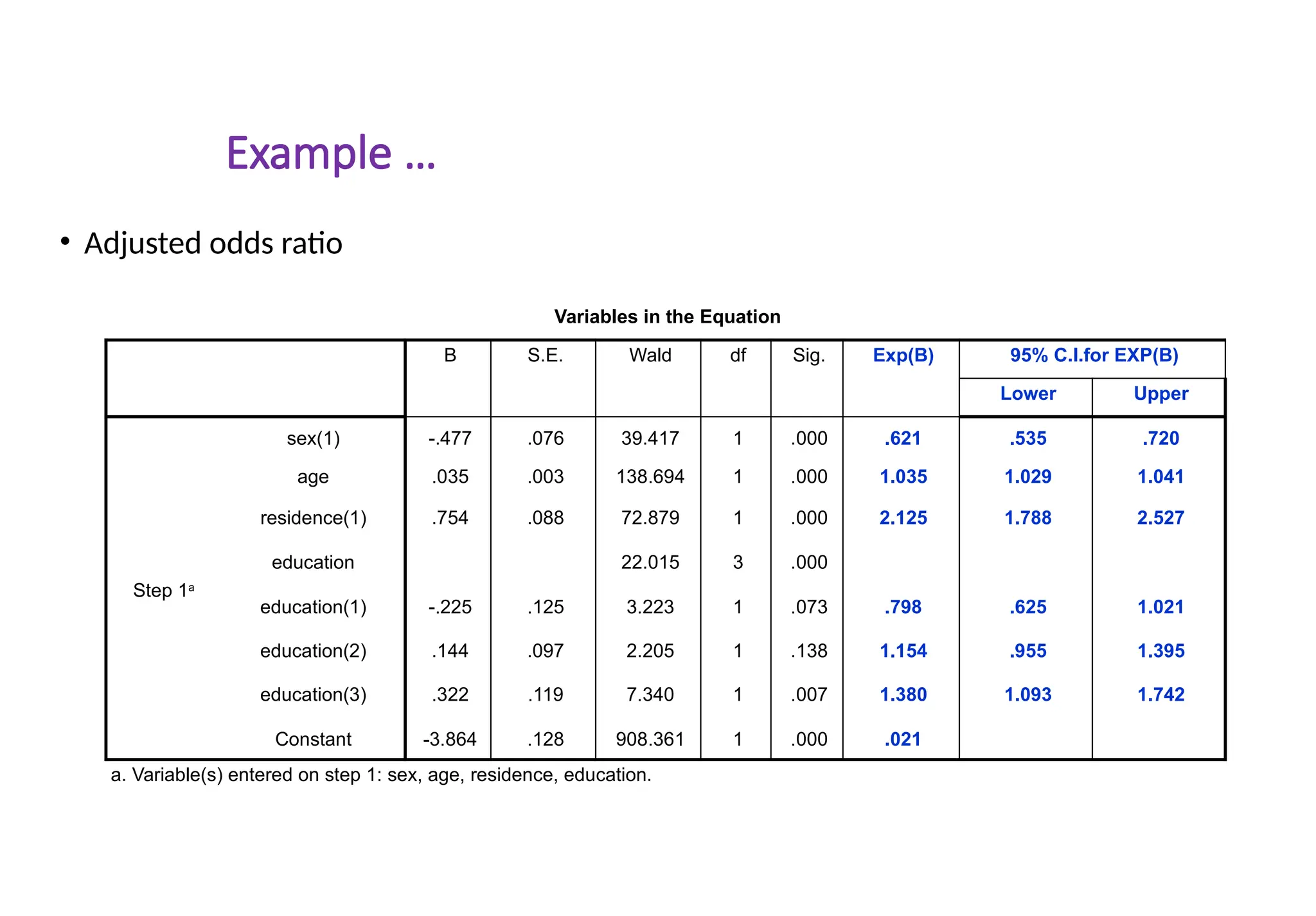
20. Example …
• For age, the crude odds ratio is
• For sex
95% Confidence Interval for
COR
Variable COR Wald Sig. Lower Bound Upper Bound
Age 1.028 102.45 .0001 1.023 1.034
Constant .027 1331.050 .000
95% Confidence Interval
for COR
Variable COR Wald Sig. Lower
Bound
Upper Bound
sex .654 34.119 .000 .567 .754
Constant .078 3573.3 .000

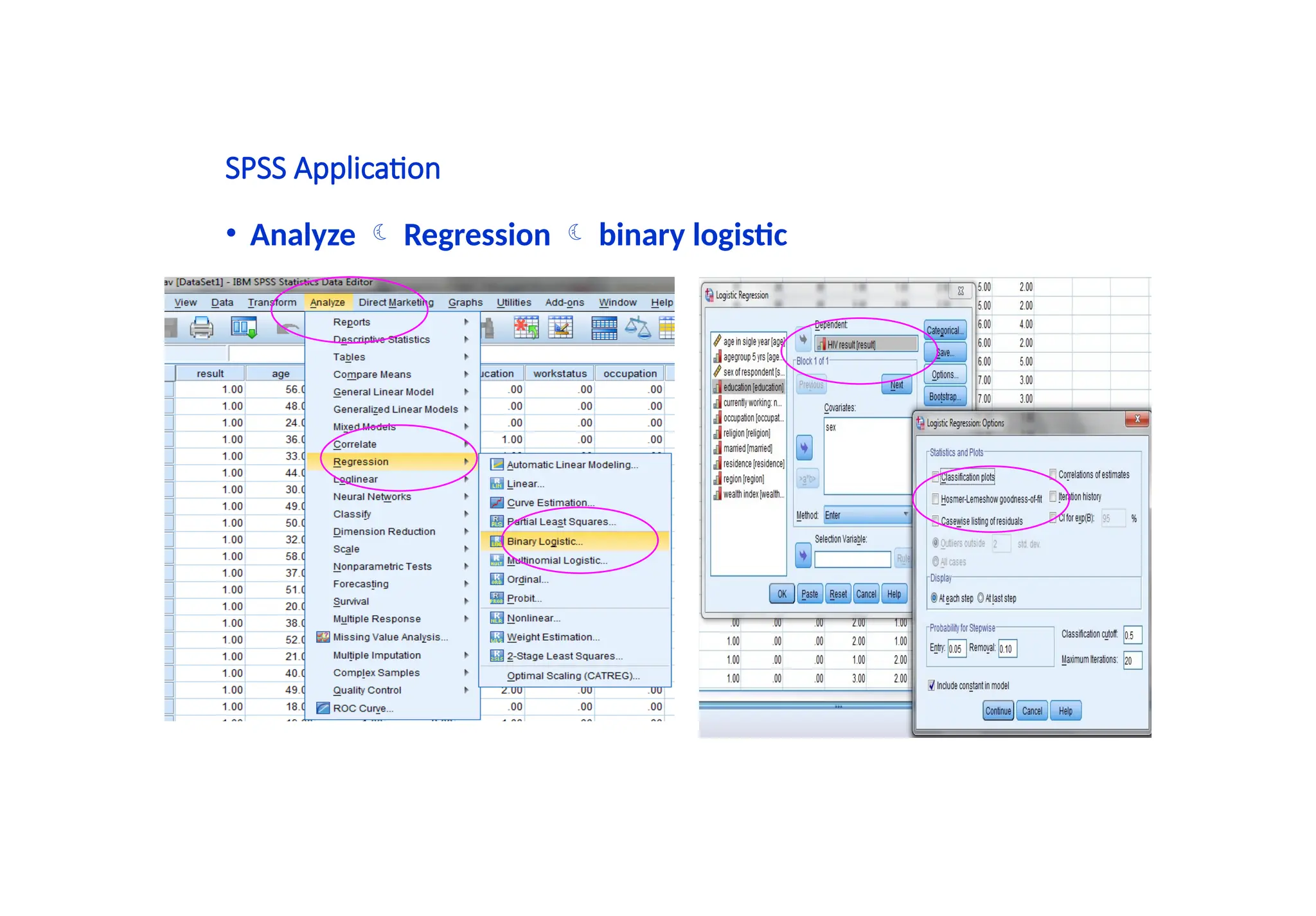
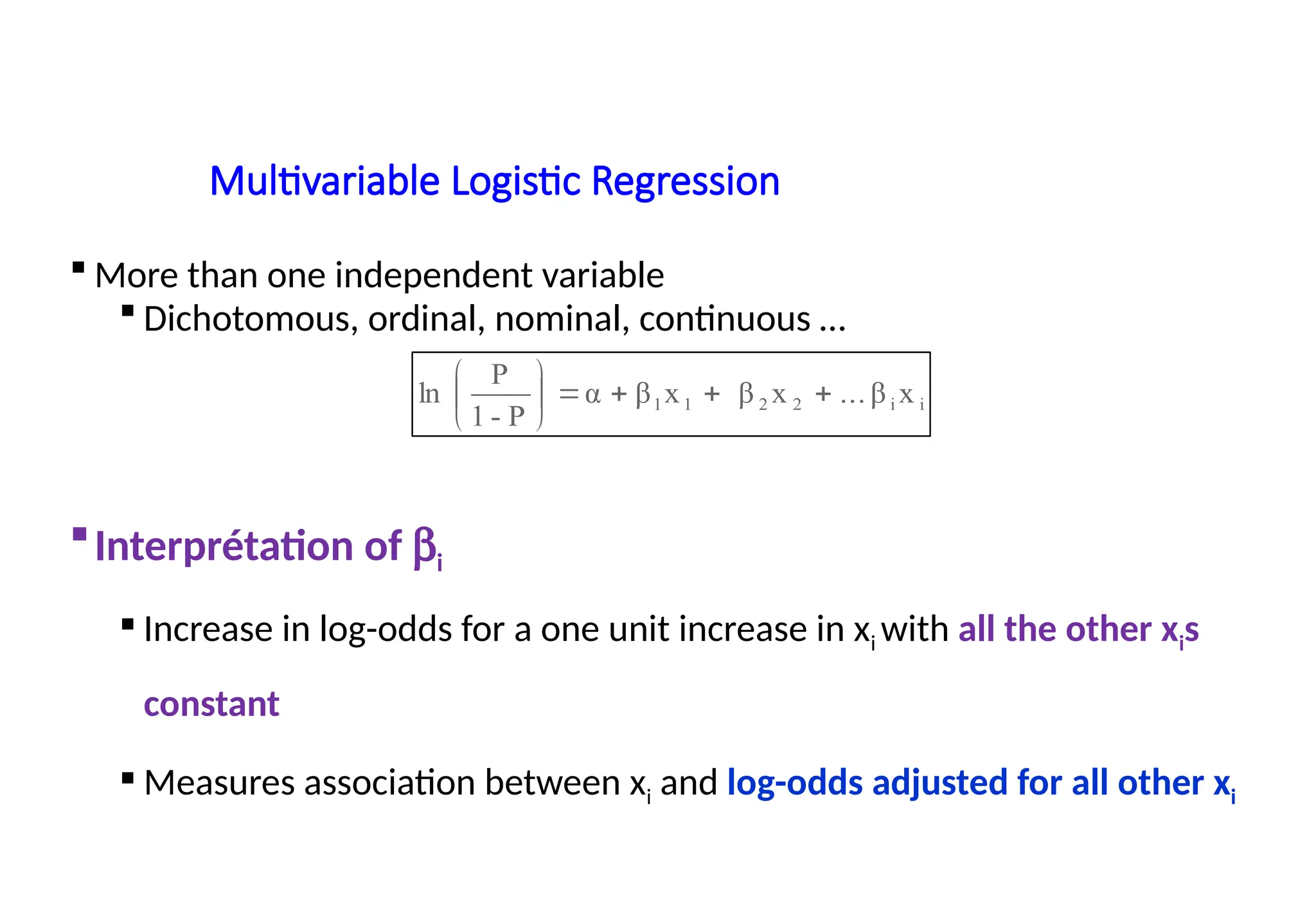
21. Multivariable Logistic Regression
 More than one independent variable
 Dichotomous, ordinal, nominal, continuous …
Interprétation of bi
 Increase in log-odds for a one unit increase in xi with all the other xis
constant
 Measures association between xi and log-odds adjusted for all other xi
i
i
2
2
1
1 x
β
...
x
β
x
β
α
P
-
1
P
ln 










22. Example …
• Adjusted odds ratio
Variables in the Equation
B S.E. Wald df Sig. Exp(B) 95% C.I.for EXP(B)
Lower Upper
Step 1a
sex(1) -.477 .076 39.417 1 .000 .621 .535 .720
age .035 .003 138.694 1 .000 1.035 1.029 1.041
residence(1) .754 .088 72.879 1 .000 2.125 1.788 2.527
education 22.015 3 .000
education(1) -.225 .125 3.223 1 .073 .798 .625 1.021
education(2) .144 .097 2.205 1 .138 1.154 .955 1.395
education(3) .322 .119 7.340 1 .007 1.380 1.093 1.742
Constant -3.864 .128 908.361 1 .000 .021
a. Variable(s) entered on step 1: sex, age, residence, education.

23. Logistic regression is a powerful statistical tool for estimating the
magnitude of the association between an exposure and a binary
outcome after adjusting simultaneously for a number of potential
confounding factors

24. Crude and Adjusted OR
Odds ratios calculated using single independent variable are
sometimes called crude odds ratios
 Adjusted for the presence of other factors in the regression equation
because the odds ratios are obtained simultaneously with all the factors
together
 Adjusted odds ratios are less affected by confounding between the factors
 Confidence intervals and p-value can be derived for odds ratio estimated
from logistic regression
 Interpretation of these is the same as in the case of the crude odds ratios

25. Hosmer and Lemeshow Test
 Hosmer -Lemeshow goodness- of - fit statistic
Used to assess whether the necessary assumptions for the
application of multivariable logistic regression are fulfilled
Computed as the Pearson chi-square from the contingency
table of observed frequencies and expected frequencies
 A good fit as measured by Hosmer and Lemeshow's test will
yield a large p-value (>0.05)

26. NEXT IS →PRACTICAL SESSION