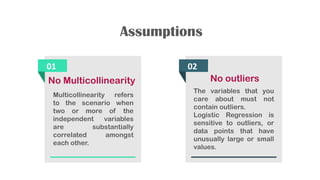
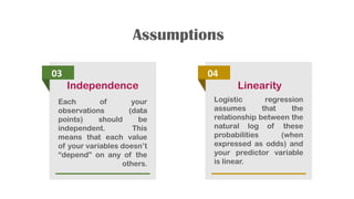
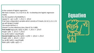
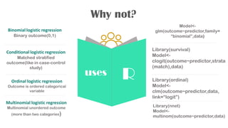
Multinomial logistic regression is an extension of binary logistic regression for outcomes with more than two unordered categories. It models the probabilities of the different categories using maximum likelihood estimation. Some examples of multinomial outcomes include blood type or candidate choice. The assumptions include no multicollinearity, no outliers, independence of observations, and linearity of relationships. The results are k-1 logistic regression models, where k is the number of categories. Interpretation includes pseudo R-square, p-values, and odds ratios. Resources for practicing on different datasets were also provided.

1. Multinomial logistic
regression
Presented
by:
Amira Badr
Aya Essam
Merit Adel
Eman Abbas
Hajer Bilal

2. Outlines
What is it?& When
to use it?
Assumptions
Data & codes
Interpretation
Why not ?
Equation

3. What is it?
when to use?
?
?
It is an extension to binary logistic
regression for multinomial responses,
where the outcome categories are
more than two and unordered.
Like binary logistic regression,
multinomial logistic regression uses
maximum likelihood estimation to
evaluate the probability of categorical
membership.

4. Multinomial Outcome examples
01
02
03
Which blood type does a
person have, given the
results of various diagnostic
tests?
Which candidate will a
person vote for, given
particular demographic
characteristics?
Entering high school
students make program
choices among general
program, Their choice might
be modeled using their
writing score and their
social economic status.

5. Assumptions
01
No Multicollinearity
Multicollinearity refers
to the scenario when
two or more of the
independent variables
are substantially
correlated amongst
each other.
02
No outliers
The variables that you
care about must not
contain outliers.
Logistic Regression is
sensitive to outliers, or
data points that have
unusually large or small
values.

6. Assumptions
03
Independence
Each of your
observations (data
points) should be
independent. This
means that each value
of your variables doesn’t
“depend” on any of the
others.
04
Linearity
Logistic regression
assumes that the
relationship between the
natural log of these
probabilities (when
expressed as odds) and
your predictor variable
is linear.

7. In the context of logistic regression:
We have 2 classes: 1 vs. 0 (or A vs. B) – to develop one logistic regression
model,
So, the equation of probability is
Log (p/ (1 – p)) = e 𝛽0 + 𝛽1𝑥1 + 𝛽2𝑥2
If we have a dependent variable which consists of 3 levels; (A, B, C,), (1, 2, 3)
we will design K model
The results will be k-1
Choose C as the reference class, then (C Vs. A &B)
First model log (p (A) / p(C)) =e 𝛽01 + 𝛽1𝑥1 + 𝛽3𝑥3
PropA = 𝛽01 + 𝛽1𝑥1 + 𝛽3𝑥3
So, (p (A) / p(C)) = exp (PropA)
Second model log (p (B) / p(C)) = e 𝛽02 + 𝛽2𝑥2 + 𝛽3𝑥3
PropB = 𝛽02 + 𝛽2𝑥2 + 𝛽3𝑥3
So, (p (B) / p(C)) = exp (PropB)
Note: p(A) + p(B) + p(C) = 1
Equation

8. our data
Covidthreat_ph
1
4
2
5
It is the dependent
Variable.
Coded as:
0=covid is not a threat.
1=covid is a minor threat.
2=covid is major threat.
Gender
agecat covidMadeUp
3
Educationlev
Independent
Variable.
Coded as:
0=male.
1=female.
Independent
Variable.
Coded as:
0=18-29.
1=30-49
2=50-64
3=65+
Independent
Variable.
Coded as:
1=less than high school
2=high school graduate
3=some college, no degree.
4=associate’s degree
5=college graduate/some
post grad.
6=postgraduate
Independent
Variable.
Coded as:
0=not at all
1=not much
2=some
3=alot

9. Simple linear regression
Outcome is a continuous
variable and one
predictor.
Multiple linear regression
Outcome is a continuous
variable and more than one
predictor.
Poisson regression
outcome variable is a count
variable.
Why not?
Model<-lm(outcome~predictor)
Model<-
glm(outcome~predictor,data,
family=“poisson”)
uses R
Model<-model<-
lm(outcome~predictor1+predictor
2+……)

10. Binomial logistic regression
Binary outcome(0,1)
Conditional logistic regression
Matched stratified
outcome(like in case-control
study)
Ordinal logistic regression
Outcome is ordered categorical
variable
Multinomial logistic regression
Multinomial unordered outcome
(more than two categories)
Why not?
Model<-
glm(outcome~predictor,family=
“binomial”,data)
Library(survival)
Model<-
clogit(outcome~predictor,strata
(match),data)
Library(nnet)
Model<-
multinom(outcome~predictor,data)
Library(ordinal)
Model<-
clm(outcome~predictor,data,
link=“logit”)
uses R

11. INTERPRETATION
pseudo R square
P values
Odds ratio

12. DATASETS FOR PRACTICING REGRESSION
https://www.kaggle.com/code/rtatman/datasets-for-regression-
analysis/notebook
https://www.r-bloggers.com/2020/05/multinomial-logistic-regression-with-r/
https://www.youtube.com/watch?v=csqgBOgVgJ4
Other datasets:
Dataset used in the lecture:

13. Thank you