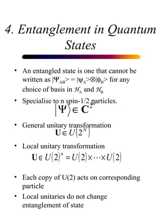
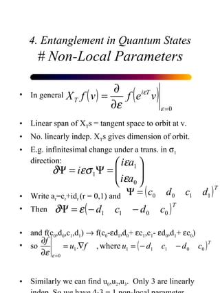
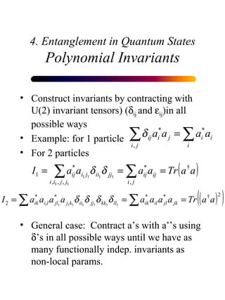
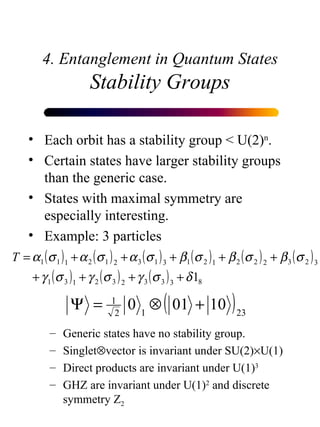
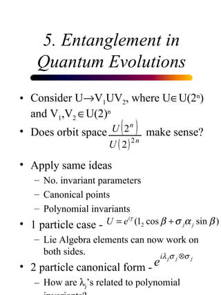
Multi-particle Entanglement in Quantum States and Evolutions Matthew Leifer - 1st Year Ph.D., Maths Dept., University of Bristol Supervisor - Dr. Noah Linden 1. Background and Motivation 2. Physical Meaning of Entanglement 3. Quantum Mechanics 4. Entanglement in Quantum States 5. Entanglement in Quantum Evolutions 6. Further Investigations
1. Background and Motivation Quantum Mechanics is weird!  role of probability  measurement problem (“collapse of wave-function”) non-local correlations (entanglement)   Quantum Mechanics is Successful! Atomic Physics and Chemistry Solid State Physics (semiconductors) Quantum Field Theory (Particle Physics) Anomalous magnetic moment of electron We do not have full control of the quantum degrees of freedom in these applications.
What happens if we can control quantum systems? Quantum Computers Feynman (1982) Holy Grails of Information Theory Polynomial time prime factorisation - Shor (1994) Perfectly secure key distribution in cryptography Other discoveries Teleportation - Bennett et al (1992) Quantum error correction - Shor (1995) These procedures use entangled states! Peter Shor Richard Feynman
3. Quantum Mechanics Measurement Quantum states, |  >, are vectors (rays) in a Hilbert space Usually we normalise s.t. <   |  > = 1  Observables are represented by Hermitian operators (i.e Q s.t. Q †  = Q) If we construct an orthonormal eigenbasis{|  i >} of Q s.t. Q|  i > =   i  |  i > then |  > =   a i  |  i > with   |a i | 2  = 1 and  a i  = <  i |  >  The possible results of measurements of Q are its eigenvalues   i The result of a measurement will be   i  with probability |a i | 2 After obtaining a value   i , the state will become |  i >
3. Quantum Mechanics Quantum Dynamics States can also evolve between measurements |  >    U |  >  Conservation of probability => states must remain normalised: <  |U † U|  > = <  |  > => U † U = 1 Quantum evolutions are unitary! Can also see this from Schrödinger eqn. In theory, can implement any unitary transformation by correct choice of H.
3. Quantum Mechanics Systems and Subsystems If we have 2 systems A and B, with Hilbert spaces  H A  and  H B  then the quantum state of the combined system is a vector in  H A  H B Example - 2 dimensional subsystems (spin-1/2 particles) H A  has basis {|0> A , |1> A } H B  has basis {|0> B , |1> B } H A  H B  has basis {|0> A  |0> B , |0> A  |1> B , |1> A  |0> B , |1> A  |1> B } or {|00>, |01>, |10>, |11>} An example vector
4. Entanglement in Quantum States An entangled state is one that cannot be written as |  AB > = |  A >  |  B > for any choice of basis in  H A  and  H B   Specialise to n spin-1/2 particles. General unitary transformation Local unitary transformation Each copy of U(2) acts on corresponding particle Local unitaries do not change entanglement of state
4. Entanglement in Quantum States # Non-Local Parameters In general Linear span of X T s = tangent space to orbit at v. No. linearly indep. X T s gives dimension of orbit. E.g. infinitesimal change under a trans. in   1  direction: Write a r =c r +id r  (r = 0,1) and  Then and f(c 0 ,d 0 ,c 1 ,d 1 )    f(c 0 -  d 1 ,d 0 +   c 1 ,c 1 -   d 0 ,d 1 +   c 0 ) so Similarly we can find u 0 ,u 2 ,u 3 .  Only 3 are linearly indep. So we have 4-3 = 1 non-local parameter
4. Entanglement in Quantum States Polynomial Invariants Construct invariants by contracting with U(2) invariant tensors) (  ij  and   ij )in all possible ways Example: for 1 particle  For 2 particles  General case:  Contract a’s with a * ’s using   ’s in all possible ways until we have as many functionally indep. invariants as non-local params.
4. Entanglement in Quantum States Stability Groups Each orbit has a stability group < U(2) n . Certain states have larger stability groups than the generic case. States with maximal symmetry are especially interesting. Example: 3 particles Generic states have no stability group. Singlet  vector is invariant under SU(2)  U(1) Direct products are invariant under U(1) 3 GHZ are invariant under U(1) 2  and discrete symmetry Z 2
5. Entanglement in Quantum Evolutions Consider U  V 1 UV 2 , where U  U(2 n ) and V 1 ,V 2   U(2) n Does orbit space    make sense? Apply same ideas No. invariant parameters Canonical points Polynomial invariants 1 particle case - Lie Algebra elements can now work on both sides. 2 particle canonical form - How are   j ’s related to polynomial invariants?
6. Future Work Density matrix formalism -  Linden, Popescu and Sudberry 1998 Find canonical forms, polynomial invariants and special orbits for n particle unitaries. Determine relation between non-locality in states and evolutions. Allow measurements.  What is the significance of  Carteret, Linden, Popescu and Sudberry (1998)

Multi-particle Entanglement in Quantum States and Evolutions

  • 1.
    Multi-particle Entanglement inQuantum States and Evolutions Matthew Leifer - 1st Year Ph.D., Maths Dept., University of Bristol Supervisor - Dr. Noah Linden 1. Background and Motivation 2. Physical Meaning of Entanglement 3. Quantum Mechanics 4. Entanglement in Quantum States 5. Entanglement in Quantum Evolutions 6. Further Investigations
  • 2.
    1. Background andMotivation Quantum Mechanics is weird! role of probability measurement problem (“collapse of wave-function”) non-local correlations (entanglement) Quantum Mechanics is Successful! Atomic Physics and Chemistry Solid State Physics (semiconductors) Quantum Field Theory (Particle Physics) Anomalous magnetic moment of electron We do not have full control of the quantum degrees of freedom in these applications.
  • 3.
    What happens ifwe can control quantum systems? Quantum Computers Feynman (1982) Holy Grails of Information Theory Polynomial time prime factorisation - Shor (1994) Perfectly secure key distribution in cryptography Other discoveries Teleportation - Bennett et al (1992) Quantum error correction - Shor (1995) These procedures use entangled states! Peter Shor Richard Feynman
  • 4.
    3. Quantum MechanicsMeasurement Quantum states, |  >, are vectors (rays) in a Hilbert space Usually we normalise s.t. <  |  > = 1 Observables are represented by Hermitian operators (i.e Q s.t. Q † = Q) If we construct an orthonormal eigenbasis{|  i >} of Q s.t. Q|  i > =  i |  i > then |  > =  a i |  i > with  |a i | 2 = 1 and a i = <  i |  > The possible results of measurements of Q are its eigenvalues  i The result of a measurement will be  i with probability |a i | 2 After obtaining a value  i , the state will become |  i >
  • 5.
    3. Quantum MechanicsQuantum Dynamics States can also evolve between measurements |  >  U |  > Conservation of probability => states must remain normalised: <  |U † U|  > = <  |  > => U † U = 1 Quantum evolutions are unitary! Can also see this from Schrödinger eqn. In theory, can implement any unitary transformation by correct choice of H.
  • 6.
    3. Quantum MechanicsSystems and Subsystems If we have 2 systems A and B, with Hilbert spaces H A and H B then the quantum state of the combined system is a vector in H A  H B Example - 2 dimensional subsystems (spin-1/2 particles) H A has basis {|0> A , |1> A } H B has basis {|0> B , |1> B } H A  H B has basis {|0> A  |0> B , |0> A  |1> B , |1> A  |0> B , |1> A  |1> B } or {|00>, |01>, |10>, |11>} An example vector
  • 7.
    4. Entanglement inQuantum States An entangled state is one that cannot be written as |  AB > = |  A >  |  B > for any choice of basis in H A and H B Specialise to n spin-1/2 particles. General unitary transformation Local unitary transformation Each copy of U(2) acts on corresponding particle Local unitaries do not change entanglement of state
  • 8.
    4. Entanglement inQuantum States # Non-Local Parameters In general Linear span of X T s = tangent space to orbit at v. No. linearly indep. X T s gives dimension of orbit. E.g. infinitesimal change under a trans. in  1 direction: Write a r =c r +id r (r = 0,1) and Then and f(c 0 ,d 0 ,c 1 ,d 1 )  f(c 0 -  d 1 ,d 0 +  c 1 ,c 1 -  d 0 ,d 1 +  c 0 ) so Similarly we can find u 0 ,u 2 ,u 3 . Only 3 are linearly indep. So we have 4-3 = 1 non-local parameter
  • 9.
    4. Entanglement inQuantum States Polynomial Invariants Construct invariants by contracting with U(2) invariant tensors) (  ij and  ij )in all possible ways Example: for 1 particle For 2 particles General case: Contract a’s with a * ’s using  ’s in all possible ways until we have as many functionally indep. invariants as non-local params.
  • 10.
    4. Entanglement inQuantum States Stability Groups Each orbit has a stability group < U(2) n . Certain states have larger stability groups than the generic case. States with maximal symmetry are especially interesting. Example: 3 particles Generic states have no stability group. Singlet  vector is invariant under SU(2)  U(1) Direct products are invariant under U(1) 3 GHZ are invariant under U(1) 2 and discrete symmetry Z 2
  • 11.
    5. Entanglement inQuantum Evolutions Consider U  V 1 UV 2 , where U  U(2 n ) and V 1 ,V 2  U(2) n Does orbit space make sense? Apply same ideas No. invariant parameters Canonical points Polynomial invariants 1 particle case - Lie Algebra elements can now work on both sides. 2 particle canonical form - How are  j ’s related to polynomial invariants?
  • 12.
    6. Future WorkDensity matrix formalism - Linden, Popescu and Sudberry 1998 Find canonical forms, polynomial invariants and special orbits for n particle unitaries. Determine relation between non-locality in states and evolutions. Allow measurements. What is the significance of Carteret, Linden, Popescu and Sudberry (1998)