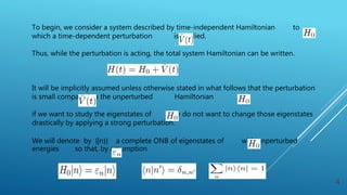
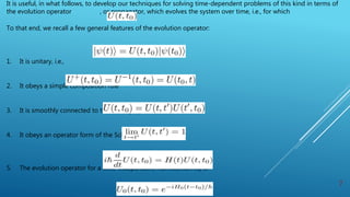
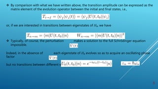
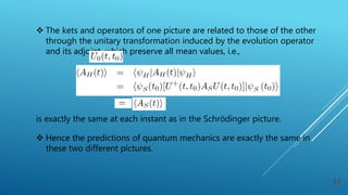
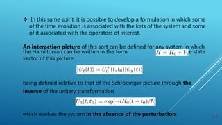
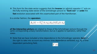
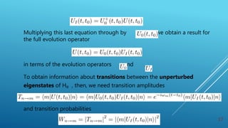
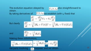
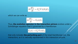
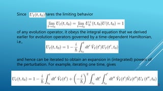
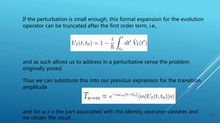
TIME-DEPENDENT PERTURBATION
BY
Zahid Mehmood
Govt. S.E. College Bahawalpur
Lecture No.2
 The methods of time-independent perturbation theory have as their goal expressions for the exact
energy eigenstates of a system in terms of those of a closely related system to which a constant
perturbation has been applied.
 We consider now a related problem, namely, that of determining the rate at which transitions occur
between energy eigenstates of a quantum system of interest as a result of a time-dependent, usually
externally applied, perturbation.
 Indeed, it is often the case that the only way of experimentally determining the structure of the energy
eigenstates of a quantum mechanical system is by perturbing it in some way.
 We know, e.g., that if a system is in an eigenstate of the Hamiltonian, then it will remain in that state for
all time. But by applying perturbations, one can induce transitions between different eigenstates of the
unperturbed Hamiltonian.
 By probing the rate at which such transitions occur, and the energies absorbed or emitted by the
system in the process, we can infer information about the states involved.
 This topic thus addresses the calculation of transition rates for such situations, as well as a number of
related problems involving time dependent perturbations.
2
 But by applying perturbations, one can induce transitions between different eigenstates of the
unperturbed Hamiltonian.
 By probing the rate at which such transitions occur, and the energies absorbed or emitted by the system
in the process, we can infer information about the states involved.
 This topic thus addresses the calculation of transition rates for such situations, as well as a number of
related problems involving time dependent perturbations.
 But by applying perturbations, one can induce transitions between different eigenstates of the
unperturbed Hamiltonian.
 By probing the rate at which such transitions occur, and the energies absorbed or emitted by the system
in the process, we can infer information about the states involved.
 This topic, therefore addresses the calculation of transition rates for such situations, as well as a number
of related problems involving time dependent perturbations.
To begin, we consider a system described by time-independent Hamiltonian to
which a time-dependent perturbation is applied.
Thus, while the perturbation is acting, the total system Hamiltonian can be written.
It will be implicitly assumed unless otherwise stated in what follows that the perturbation
is small compared to the unperturbed Hamiltonian
if we want to study the eigenstates of we do not want to change those eigenstates
drastically by applying a strong perturbation.
We will denote by {|n〉} a complete ONB of eigenstates of with unperturbed
energies so that, by assumption
4
Our general goal: is to calculate the amplitude (or probability) to find
the system in a given final state at time t if it was known to be in a state
at some initial time t₀.
Implicit in this statement is the idea that we are going to let the system evolve from
until time t and then make a measurement of some observable of which is an
eigenstate.
A little less generally, if the system was initially in the unperturbed eigenstate of
H₀ at t₀, we wish to find the amplitude that it will be left in (or will be found
have made a transition to) the unperturbed eigenstate at time
t > t₀, where now the measurement will be that of the unperturbed Hamiltonian itself.
5
 We note in passing that if we could solve the full Schrödinger equation
In the presence of the perturbation, for the initial condition of interest,
the solution to the general problem would be solved.
The corresponding transition amplitude would then just be the inner product
 and the transition probability would be the squared magnitude of the transition
amplitude.
It is useful, in what follows, to develop our techniques for solving time-dependent problems of this kind in terms of
the evolution operator , or propagator, which evolves the system over time, i.e., for which
To that end, we recall a few general features of the evolution operator:
1. It is unitary, i.e.,
2. It obeys a simple composition rule
3. It is smoothly connected to the identity operator
4. It obeys an operator form of the Schrödinger equation
5. The evolution operator for a time-independent Hamiltonian H₀ is
7
 By comparison with what we have written above, the transition amplitude can be expressed as the
matrix element of the evolution operator between the initial and final states, i.e.,
or, if we are interested in transitions between eigenstates of H₀, we have
 Typically, of course, the perturbation makes a solution to the full Schrödinger equation
impossible.
Indeed, in the absence of each eigenstate of H₀ evolves so as to acquire an oscillating phase
factor
but no transitions between different eigenstates occur.
8
 It is the perturbation that allows the system to evolve into a mixture of
unperturbed states, an evolution that is viewed as inducing transitions between
them.
 Our goal, then, is to develop a general expansion for the full evolution operator
in powers of the perturbation.
 To this end, it is useful to observe that the "fast" unperturbed part of the evolution
of the system is not of any real interest, involving as it does all of the unperturbed
Eigen energies and oscillating phase factors of the system.
 It would be convenient, therefore, to transform to a set of variables that evolve, in a
certain sense, along with the unperturbed system, so that we can focus on the
relatively slow part of the evolution induced by the weak externally applied
perturbation, without worrying about all the rapid oscillation of the phase factors
associated with the part of the evolution arising from H₀.
9
 The idea here is similar to transforming to a rotating coordinate system
to ease the solution of simple mechanical problems.
 As it turns out, we can formally eliminate the fast evolution generated by
H₀ by working in the something called the interaction picture.
 As it turns out, we developed our postulates of quantum mechanics
working implicitly in what is called the Schrödinger picture in which
the state of the system evolves in time

 while fundamental observables of the system are usually associated
with time-independent Hermitian operators [except for
explicitly time-dependent perturbations like V(t), which are constructed
out of time-independent observables)
10
 In the Schrödinger picture mean values of even time-independent
observables can evolve in time
due to the evolution of the state itself.
 But we can always express these in terms of expectation values taken
with respect to the initial state by expressing the state at time t to the
initial state using the evolution operator.
11
 By contrast, it is possible to develop a different formulation of quantum
mechanics, referred to as the Heisenberg picture, in which the
Heisenberg state of the system
remains fixed in time, and equal to its initial value, which is the same as in
the Schrödinger picture.
 But in the Heisenberg picture fundamental observables are now
associated with Heisenberg operators that evolve in time, and which
are defined in terms of the corresponding Schrödinger operators
through the relation
.
12
 The kets and operators of one picture are related to those of the other
through the unitary transformation induced by the evolution operator
and its adjoint, which preserve all mean values, i.e.,
is exactly the same at each instant as in the Schrödinger picture.
 Hence the predictions of quantum mechanics are exactly the same in
these two different pictures.
13
 In this same spirit, it is possible to develop a formulation in which some
of the time evolution is associated with the kets of the system and some
of it associated with the operators of interest.
An interaction picture of this sort can be defined for any system in which
the Hamiltonian can be written in the form with the state
vector of this picture
being defined relative to that of the Schrödinger picture through the
inverse of the unitary transformation
which evolves the system in the absence of the perturbation. 14
 This form for the state vector suggests that the inverse (or adjoint) operator U⁺ acts on
the fully-evolving state vector of the Schrödinger picture to "back out" or undo the
fast evolution associated with the unperturbed part of the Hamiltonian.
In a similar fashion, the operators
of the interaction picture are related to those of the Schrödinger picture through the
same corresponding unitary transformation, but as it applies to operators, rather than
states.
 Note that we have included a time dependence in the Schrodinger operator As(t) on
the right to take into account any intrinsic time dependence exhibited, e.g., by a time
dependent perturbing field.
15
Naturally, we can define an evolution operator for the interaction picture
that evolves the state vector in time, according to the relation
where is the same as since .
Using the definitions given above we deduce that since
which makes it clear that
16
Multiplying this last equation through by we obtain a result for
the full evolution operator
in terms of the evolution operators and .
To obtain information about transitions between the unperturbed
eigenstates of H₀ , then, we need transition amplitudes
and transition probabilities
17
The evolution equation obeyed by is also straightforward to
obtain.
By taking derivatives of we establish (with t₀ fixed) that
But clearly
and
Making these substitutions,
the parts involving disappear, and we obtain . . . 18
which we can write as
Thus, the evolution operator in the interaction picture evolves under a
Schrödinger equation that is governed by a Hamiltonian
that only includes the perturbing part of the total Hamiltonian (i.e., the
interaction), as it is naturally represented in this interaction picture.
19
Since s hares the limiting behavior
of any evolution operator, it obeys the integral equation that we derived
earlier for evolution operators governed by a time-dependent Hamiltonian,
i.e.,
and hence can be iterated to obtain an expansion in (integrated) powers of
the perturbation. For example, iterating one time, gives
20
If the perturbation is small enough, this formal expansion for the evolution
operator can be truncated after the first order term, i.e.,
and as such allows us to address in a perturbative sense the problem
originally posed.
Thus we can substitute this into our previous expression for the transition
amplitude
and for m ≠ n the part associated with the identity operator vanishes and
we obtain the result . . .
21
where is the Bohr frequency associated with the
transition between levels n and m.
22
Taking the squared magnitude of this gives the basic result of time
dependent perturbation theory, namely the transition probability
between unperturbed eigenstates of , correct to lowest non-trivial
order in the perturbation.
In the next segment, we apply this formula to a so-called pulsed
perturbation that vanishes at times in the past, and times in the future,
but is non-zero over some time interval, during which it induces transitions
in the system of interest.
23

Time dependent perturbations

  • 1.
    TIME-DEPENDENT PERTURBATION BY Zahid Mehmood Govt.S.E. College Bahawalpur Lecture No.2
  • 2.
     The methodsof time-independent perturbation theory have as their goal expressions for the exact energy eigenstates of a system in terms of those of a closely related system to which a constant perturbation has been applied.  We consider now a related problem, namely, that of determining the rate at which transitions occur between energy eigenstates of a quantum system of interest as a result of a time-dependent, usually externally applied, perturbation.  Indeed, it is often the case that the only way of experimentally determining the structure of the energy eigenstates of a quantum mechanical system is by perturbing it in some way.  We know, e.g., that if a system is in an eigenstate of the Hamiltonian, then it will remain in that state for all time. But by applying perturbations, one can induce transitions between different eigenstates of the unperturbed Hamiltonian.  By probing the rate at which such transitions occur, and the energies absorbed or emitted by the system in the process, we can infer information about the states involved.  This topic thus addresses the calculation of transition rates for such situations, as well as a number of related problems involving time dependent perturbations. 2
  • 3.
     But byapplying perturbations, one can induce transitions between different eigenstates of the unperturbed Hamiltonian.  By probing the rate at which such transitions occur, and the energies absorbed or emitted by the system in the process, we can infer information about the states involved.  This topic thus addresses the calculation of transition rates for such situations, as well as a number of related problems involving time dependent perturbations.  But by applying perturbations, one can induce transitions between different eigenstates of the unperturbed Hamiltonian.  By probing the rate at which such transitions occur, and the energies absorbed or emitted by the system in the process, we can infer information about the states involved.  This topic, therefore addresses the calculation of transition rates for such situations, as well as a number of related problems involving time dependent perturbations.
  • 4.
    To begin, weconsider a system described by time-independent Hamiltonian to which a time-dependent perturbation is applied. Thus, while the perturbation is acting, the total system Hamiltonian can be written. It will be implicitly assumed unless otherwise stated in what follows that the perturbation is small compared to the unperturbed Hamiltonian if we want to study the eigenstates of we do not want to change those eigenstates drastically by applying a strong perturbation. We will denote by {|n〉} a complete ONB of eigenstates of with unperturbed energies so that, by assumption 4
  • 5.
    Our general goal:is to calculate the amplitude (or probability) to find the system in a given final state at time t if it was known to be in a state at some initial time t₀. Implicit in this statement is the idea that we are going to let the system evolve from until time t and then make a measurement of some observable of which is an eigenstate. A little less generally, if the system was initially in the unperturbed eigenstate of H₀ at t₀, we wish to find the amplitude that it will be left in (or will be found have made a transition to) the unperturbed eigenstate at time t > t₀, where now the measurement will be that of the unperturbed Hamiltonian itself. 5
  • 6.
     We notein passing that if we could solve the full Schrödinger equation In the presence of the perturbation, for the initial condition of interest, the solution to the general problem would be solved. The corresponding transition amplitude would then just be the inner product  and the transition probability would be the squared magnitude of the transition amplitude.
  • 7.
    It is useful,in what follows, to develop our techniques for solving time-dependent problems of this kind in terms of the evolution operator , or propagator, which evolves the system over time, i.e., for which To that end, we recall a few general features of the evolution operator: 1. It is unitary, i.e., 2. It obeys a simple composition rule 3. It is smoothly connected to the identity operator 4. It obeys an operator form of the Schrödinger equation 5. The evolution operator for a time-independent Hamiltonian H₀ is 7
  • 8.
     By comparisonwith what we have written above, the transition amplitude can be expressed as the matrix element of the evolution operator between the initial and final states, i.e., or, if we are interested in transitions between eigenstates of H₀, we have  Typically, of course, the perturbation makes a solution to the full Schrödinger equation impossible. Indeed, in the absence of each eigenstate of H₀ evolves so as to acquire an oscillating phase factor but no transitions between different eigenstates occur. 8
  • 9.
     It isthe perturbation that allows the system to evolve into a mixture of unperturbed states, an evolution that is viewed as inducing transitions between them.  Our goal, then, is to develop a general expansion for the full evolution operator in powers of the perturbation.  To this end, it is useful to observe that the "fast" unperturbed part of the evolution of the system is not of any real interest, involving as it does all of the unperturbed Eigen energies and oscillating phase factors of the system.  It would be convenient, therefore, to transform to a set of variables that evolve, in a certain sense, along with the unperturbed system, so that we can focus on the relatively slow part of the evolution induced by the weak externally applied perturbation, without worrying about all the rapid oscillation of the phase factors associated with the part of the evolution arising from H₀. 9
  • 10.
     The ideahere is similar to transforming to a rotating coordinate system to ease the solution of simple mechanical problems.  As it turns out, we can formally eliminate the fast evolution generated by H₀ by working in the something called the interaction picture.  As it turns out, we developed our postulates of quantum mechanics working implicitly in what is called the Schrödinger picture in which the state of the system evolves in time   while fundamental observables of the system are usually associated with time-independent Hermitian operators [except for explicitly time-dependent perturbations like V(t), which are constructed out of time-independent observables) 10
  • 11.
     In theSchrödinger picture mean values of even time-independent observables can evolve in time due to the evolution of the state itself.  But we can always express these in terms of expectation values taken with respect to the initial state by expressing the state at time t to the initial state using the evolution operator. 11
  • 12.
     By contrast,it is possible to develop a different formulation of quantum mechanics, referred to as the Heisenberg picture, in which the Heisenberg state of the system remains fixed in time, and equal to its initial value, which is the same as in the Schrödinger picture.  But in the Heisenberg picture fundamental observables are now associated with Heisenberg operators that evolve in time, and which are defined in terms of the corresponding Schrödinger operators through the relation . 12
  • 13.
     The ketsand operators of one picture are related to those of the other through the unitary transformation induced by the evolution operator and its adjoint, which preserve all mean values, i.e., is exactly the same at each instant as in the Schrödinger picture.  Hence the predictions of quantum mechanics are exactly the same in these two different pictures. 13
  • 14.
     In thissame spirit, it is possible to develop a formulation in which some of the time evolution is associated with the kets of the system and some of it associated with the operators of interest. An interaction picture of this sort can be defined for any system in which the Hamiltonian can be written in the form with the state vector of this picture being defined relative to that of the Schrödinger picture through the inverse of the unitary transformation which evolves the system in the absence of the perturbation. 14
  • 15.
     This formfor the state vector suggests that the inverse (or adjoint) operator U⁺ acts on the fully-evolving state vector of the Schrödinger picture to "back out" or undo the fast evolution associated with the unperturbed part of the Hamiltonian. In a similar fashion, the operators of the interaction picture are related to those of the Schrödinger picture through the same corresponding unitary transformation, but as it applies to operators, rather than states.  Note that we have included a time dependence in the Schrodinger operator As(t) on the right to take into account any intrinsic time dependence exhibited, e.g., by a time dependent perturbing field. 15
  • 16.
    Naturally, we candefine an evolution operator for the interaction picture that evolves the state vector in time, according to the relation where is the same as since . Using the definitions given above we deduce that since which makes it clear that 16
  • 17.
    Multiplying this lastequation through by we obtain a result for the full evolution operator in terms of the evolution operators and . To obtain information about transitions between the unperturbed eigenstates of H₀ , then, we need transition amplitudes and transition probabilities 17
  • 18.
    The evolution equationobeyed by is also straightforward to obtain. By taking derivatives of we establish (with t₀ fixed) that But clearly and Making these substitutions, the parts involving disappear, and we obtain . . . 18
  • 19.
    which we canwrite as Thus, the evolution operator in the interaction picture evolves under a Schrödinger equation that is governed by a Hamiltonian that only includes the perturbing part of the total Hamiltonian (i.e., the interaction), as it is naturally represented in this interaction picture. 19
  • 20.
    Since s haresthe limiting behavior of any evolution operator, it obeys the integral equation that we derived earlier for evolution operators governed by a time-dependent Hamiltonian, i.e., and hence can be iterated to obtain an expansion in (integrated) powers of the perturbation. For example, iterating one time, gives 20
  • 21.
    If the perturbationis small enough, this formal expansion for the evolution operator can be truncated after the first order term, i.e., and as such allows us to address in a perturbative sense the problem originally posed. Thus we can substitute this into our previous expression for the transition amplitude and for m ≠ n the part associated with the identity operator vanishes and we obtain the result . . . 21
  • 22.
    where is theBohr frequency associated with the transition between levels n and m. 22
  • 23.
    Taking the squaredmagnitude of this gives the basic result of time dependent perturbation theory, namely the transition probability between unperturbed eigenstates of , correct to lowest non-trivial order in the perturbation. In the next segment, we apply this formula to a so-called pulsed perturbation that vanishes at times in the past, and times in the future, but is non-zero over some time interval, during which it induces transitions in the system of interest. 23