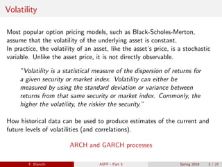
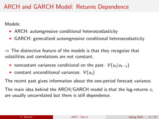
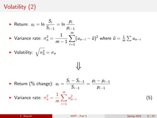
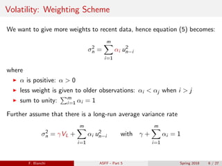
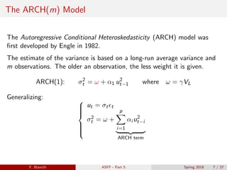
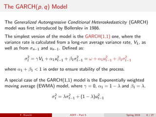
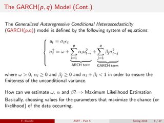
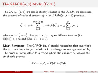
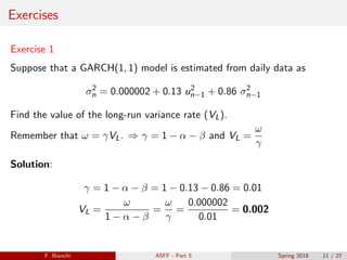
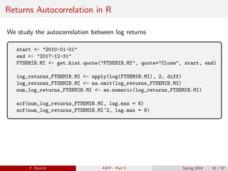
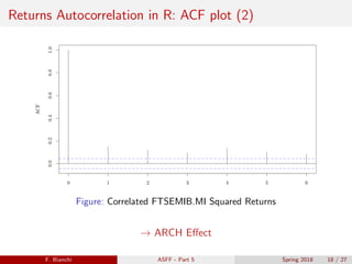
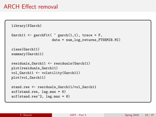
Definition of Co-integration .
Different Approaches of Co-integration.
Johansen and Juselius (J.J) Co-integration.
Error Correction Model (ECM).
Interpretation of ECM term.
Long – Run Co-integration Equation.
Definition of Co-integration .
Different Approaches of Co-integration.
Johansen and Juselius (J.J) Co-integration.
Error Correction Model (ECM).
Interpretation of ECM term.
Long – Run Co-integration Equation.
Time Series basic concepts and ARIMA family of models. There is an associated video session along with code in github: https://github.com/bhaskatripathi/timeseries-autoregressive-models
https://drive.google.com/file/d/1yXffXQlL6i4ufQLSpFFrJgymhHNXL1Mf/view?usp=sharing
Unit Root Test
1: What is unit root?
2: How to check unit root?
3: Types of unit root test
4: Dickey fuller
5: Augmented dickey fuller
6: Phillip perron
7: Testing Unit Root on E-views
Banque de France's Workshop on Granularity: Basile Grassi's slides, June 2016 Soledad Zignago
Large Firm Dynamics and the Business Cycle, slides by Basile Grassi (University of Oxford & Nuffield College), joint work with Vasco Carvalho (University of Cambridge & CREI, University Pompeu Fabra GSE & CEPR), at the Banque de France and Sciences Po joint workshop on Granularity of Macroeconomics Fluctuations, 24 June 2016. Slides of presentations & discussions are available online: https://www.banque-france.fr/en/economics-statistics/research/seminars-and-symposiums/research-workshop-on-the-granularity-of-macroeconomic-fluctuations-where-do-we-stand.html
Analyzing high-frequency time series is increasingly useful with the current explosion in the availability of these data in several application areas, including but not limited to, climate, finance, health analytics, transportation, etc. This talk will give an overview of two statistical frameworks that could be useful for analyzing high-frequency financial time series leading to quantification of financial risk. These include a distribution free approach using penalized estimating functions for modeling inter-event durations and an approximate Bayesian approach for modeling counts of events in regular intervals. A few other potentially useful lines of research in this area will also be introduced.
Pricing average price advertising options when underlying spot market prices ...Bowei Chen
Advertising options have been recently studied as a special type of guaranteed contracts in online advertising, which are an alternative sales mechanism to real-time auctions. An advertising option is a contract which gives its buyer a right but not obligation to enter into transactions to purchase page views or link clicks at one or multiple pre-specified prices in a specific future period. Different from typical guaranteed contracts, the option buyer pays a lower upfront fee but can have greater flexibility and more control of advertising. Many studies on advertising options so far have been restricted to the situations where the option payoff is determined by the underlying spot market price at a specific time point and the price evolution over time is assumed to be continuous. The former leads to a biased calculation of option payoff and the latter is invalid empirically for many online advertising slots. This paper addresses these two limitations by proposing a new advertising option pricing framework. First, the option payoff is calculated based on an average price over a specific future period. Therefore, the option becomes path-dependent. The average price is measured by the power mean, which contains several existing option payoff functions as its special cases. Second, jump-diffusion stochastic models are used to describe the movement of the underlying spot market price, which incorporate several important statistical properties including jumps and spikes, non-normality, and absence of autocorrelations. A general option pricing algorithm is obtained based on Monte Carlo simulation. In addition, an explicit pricing formula is derived for the case when the option payoff is based on the geometric mean. This pricing formula is also a generalized version of several other option pricing models discussed in related studies.
"Correlated Volatility Shocks" by Dr. Xiao Qiao, Researcher at SummerHaven In...Quantopian
Commonality in idiosyncratic volatility cannot be completely explained by time-varying volatility. After removing the effects of time-varying volatility, idiosyncratic volatility innovations are still positively correlated. This result suggests correlated volatility shocks contribute to the comovement in idiosyncratic volatility.
Motivated by this fact, we propose the Dynamic Factor Correlation (DFC) model, which fits the data well and captures the cross-sectional correlations in idiosyncratic volatility innovations. We decompose the common factor in idiosyncratic volatility (CIV) of Herskovic et al. (2016) into the volatility innovation factor (VIN) and time-varying volatility factor (TVV). Whereas VIN is associated with strong variation in average returns, TVV is only weakly priced in the cross section
A strategy that takes a long position in the portfolio with the lowest VIN and TVV betas, and a short position in the portfolio with the highest VIN and TVV betas earns average returns of 8.0% per year.
how to sell pi coins on Bitmart crypto exchangeDOT TECH
Yes. Pi network coins can be exchanged but not on bitmart exchange. Because pi network is still in the enclosed mainnet. The only way pioneers are able to trade pi coins is by reselling the pi coins to pi verified merchants.
A verified merchant is someone who buys pi network coins and resell it to exchanges looking forward to hold till mainnet launch.
I will leave the telegram contact of my personal pi merchant to trade with.
@Pi_vendor_247
how can i use my minded pi coins I need some funds.DOT TECH
If you are interested in selling your pi coins, i have a verified pi merchant, who buys pi coins and resell them to exchanges looking forward to hold till mainnet launch.
Because the core team has announced that pi network will not be doing any pre-sale. The only way exchanges like huobi, bitmart and hotbit can get pi is by buying from miners.
Now a merchant stands in between these exchanges and the miners. As a link to make transactions smooth. Because right now in the enclosed mainnet you can't sell pi coins your self. You need the help of a merchant,
i will leave the telegram contact of my personal pi merchant below. 👇 I and my friends has traded more than 3000pi coins with him successfully.
@Pi_vendor_247
If you are looking for a pi coin investor. Then look no further because I have the right one he is a pi vendor (he buy and resell to whales in China). I met him on a crypto conference and ever since I and my friends have sold more than 10k pi coins to him And he bought all and still want more. I will drop his telegram handle below just send him a message.
@Pi_vendor_247
What price will pi network be listed on exchangesDOT TECH
The rate at which pi will be listed is practically unknown. But due to speculations surrounding it the predicted rate is tends to be from 30$ — 50$.
So if you are interested in selling your pi network coins at a high rate tho. Or you can't wait till the mainnet launch in 2026. You can easily trade your pi coins with a merchant.
A merchant is someone who buys pi coins from miners and resell them to Investors looking forward to hold massive quantities till mainnet launch.
I will leave the telegram contact of my personal pi vendor to trade with.
@Pi_vendor_247
when will pi network coin be available on crypto exchange.DOT TECH
There is no set date for when Pi coins will enter the market.
However, the developers are working hard to get them released as soon as possible.
Once they are available, users will be able to exchange other cryptocurrencies for Pi coins on designated exchanges.
But for now the only way to sell your pi coins is through verified pi vendor.
Here is the telegram contact of my personal pi vendor
@Pi_vendor_247
What website can I sell pi coins securely.DOT TECH
Currently there are no website or exchange that allow buying or selling of pi coins..
But you can still easily sell pi coins, by reselling it to exchanges/crypto whales interested in holding thousands of pi coins before the mainnet launch.
Who is a pi merchant?
A pi merchant is someone who buys pi coins from miners and resell to these crypto whales and holders of pi..
This is because pi network is not doing any pre-sale. The only way exchanges can get pi is by buying from miners and pi merchants stands in between the miners and the exchanges.
How can I sell my pi coins?
Selling pi coins is really easy, but first you need to migrate to mainnet wallet before you can do that. I will leave the telegram contact of my personal pi merchant to trade with.
Tele-gram.
@Pi_vendor_247
how to sell pi coins in South Korea profitably.DOT TECH
Yes. You can sell your pi network coins in South Korea or any other country, by finding a verified pi merchant
What is a verified pi merchant?
Since pi network is not launched yet on any exchange, the only way you can sell pi coins is by selling to a verified pi merchant, and this is because pi network is not launched yet on any exchange and no pre-sale or ico offerings Is done on pi.
Since there is no pre-sale, the only way exchanges can get pi is by buying from miners. So a pi merchant facilitates these transactions by acting as a bridge for both transactions.
How can i find a pi vendor/merchant?
Well for those who haven't traded with a pi merchant or who don't already have one. I will leave the telegram id of my personal pi merchant who i trade pi with.
Tele gram: @Pi_vendor_247
#pi #sell #nigeria #pinetwork #picoins #sellpi #Nigerian #tradepi #pinetworkcoins #sellmypi
Lecture slide titled Fraud Risk Mitigation, Webinar Lecture Delivered at the Society for West African Internal Audit Practitioners (SWAIAP) on Wednesday, November 8, 2023.
how to sell pi coins effectively (from 50 - 100k pi)DOT TECH
Anywhere in the world, including Africa, America, and Europe, you can sell Pi Network Coins online and receive cash through online payment options.
Pi has not yet been launched on any exchange because we are currently using the confined Mainnet. The planned launch date for Pi is June 28, 2026.
Reselling to investors who want to hold until the mainnet launch in 2026 is currently the sole way to sell.
Consequently, right now. All you need to do is select the right pi network provider.
Who is a pi merchant?
An individual who buys coins from miners on the pi network and resells them to investors hoping to hang onto them until the mainnet is launched is known as a pi merchant.
debuts.
I'll provide you the Telegram username
@Pi_vendor_247
BYD SWOT Analysis and In-Depth Insights 2024.pptxmikemetalprod
Indepth analysis of the BYD 2024
BYD (Build Your Dreams) is a Chinese automaker and battery manufacturer that has snowballed over the past two decades to become a significant player in electric vehicles and global clean energy technology.
This SWOT analysis examines BYD's strengths, weaknesses, opportunities, and threats as it competes in the fast-changing automotive and energy storage industries.
Founded in 1995 and headquartered in Shenzhen, BYD started as a battery company before expanding into automobiles in the early 2000s.
Initially manufacturing gasoline-powered vehicles, BYD focused on plug-in hybrid and fully electric vehicles, leveraging its expertise in battery technology.
Today, BYD is the world’s largest electric vehicle manufacturer, delivering over 1.2 million electric cars globally. The company also produces electric buses, trucks, forklifts, and rail transit.
On the energy side, BYD is a major supplier of rechargeable batteries for cell phones, laptops, electric vehicles, and energy storage systems.
The Evolution of Non-Banking Financial Companies (NBFCs) in India: Challenges...beulahfernandes8
Role in Financial System
NBFCs are critical in bridging the financial inclusion gap.
They provide specialized financial services that cater to segments often neglected by traditional banks.
Economic Impact
NBFCs contribute significantly to India's GDP.
They support sectors like micro, small, and medium enterprises (MSMEs), housing finance, and personal loans.
Seminar: Gender Board Diversity through Ownership NetworksGRAPE
Seminar on gender diversity spillovers through ownership networks at FAME|GRAPE. Presenting novel research. Studies in economics and management using econometrics methods.
Turin Startup Ecosystem 2024 - Ricerca sulle Startup e il Sistema dell'Innov...Quotidiano Piemontese
Turin Startup Ecosystem 2024
Una ricerca de il Club degli Investitori, in collaborazione con ToTeM Torino Tech Map e con il supporto della ESCP Business School e di Growth Capital
how to sell pi coins in all Africa Countries.DOT TECH
Yes. You can sell your pi network for other cryptocurrencies like Bitcoin, usdt , Ethereum and other currencies And this is done easily with the help from a pi merchant.
What is a pi merchant ?
Since pi is not launched yet in any exchange. The only way you can sell right now is through merchants.
A verified Pi merchant is someone who buys pi network coins from miners and resell them to investors looking forward to hold massive quantities of pi coins before mainnet launch in 2026.
I will leave the telegram contact of my personal pi merchant to trade with.
@Pi_vendor_247
1. Part 5: Advanced Topics
Applied Statistics for Finance
Professor Asmerilda Hitaj
asmerilda.hitaj1@unimib.it
April 10, 2018
A. Hitaj ASFF - Part 5 Spring 2018 1 / 27
2. ARCH Processes
Applied Statistics for Finance
Francesco Bianchi
francesco.bianchi04@icatt.it
April 10, 2018
F. Bianchi ASFF - Part 5 Spring 2018 2 / 27
3. Volatility
Most popular option pricing models, such as Black-Scholes-Merton,
assume that the volatility of the underlying asset is constant.
In practice, the volatility of an asset, like the asset’s price, is a stochastic
variable. Unlike the asset price, it is not directly observable.
”Volatility is a statistical measure of the dispersion of returns for
a given security or market index. Volatility can either be
measured by using the standard deviation or variance between
returns from that same security or market index. Commonly, the
higher the volatility, the riskier the security.”
How historical data can be used to produce estimates of the current and
future levels of volatilities (and correlations).
ARCH and GARCH processes
F. Bianchi ASFF - Part 5 Spring 2018 3 / 27
4. ARCH and GARCH Model: Returns Dependence
Models:
ARCH: autoregressive conditional heteroscedasticity
GARCH: generalized autoregressive conditional heteroscedasticity
⇒ The distinctive feature of the models is that they recognize that
volatilities and correlations are not constant.
noncostant variances conditional on the past: V (ut|ut−1)
constant unconditional variances: V (ut)
The recent past gives information about the one-period forecast variance.
The main idea behind the ARCH/GARCH model is that the log-returns rt
are usually uncorrelated but there is still dependence.
F. Bianchi ASFF - Part 5 Spring 2018 4 / 27
5. Volatility (2)
Return: ui = ln
Si
Si−1
= ln
pi
pi−1
Variance rate: σ2
n =
1
m − 1
m
i=1
(un−i − ¯u)2
where ¯u = 1
m un−i
Volatility: σ2
n = σn
⇓
Return (% change): ui =
Si − Si−1
Si−1
=
pi − pi−1
pi−1
Variance rate: σ2
n =
1
m
m
i=1
u2
n−i (5)
F. Bianchi ASFF - Part 5 Spring 2018 5 / 27
6. Volatility: Weighting Scheme
We want to give more weights to recent data, hence equation (5) becomes:
σ2
n =
m
i=1
αi u2
n−i
where
α is positive: α > 0
less weight is given to older observations: αi < αj when i > j
sum to unity: m
i=1 αi = 1
Further assume that there is a long-run average variance rate
σ2
n = γVL +
m
i=1
αi u2
n−i with γ +
m
i=1
αi = 1
F. Bianchi ASFF - Part 5 Spring 2018 6 / 27
7. The ARCH(m) Model
The Autoregressive Conditional Heteroskedasticity (ARCH) model was
first developed by Engle in 1982.
The estimate of the variance is based on a long-run average variance and
m observations. The older an observation, the less weight it is given.
ARCH(1): σ2
t = ω + α1 u2
t−1 where ω = γVL
Generalizing:
ut = σt t
σ2
t = ω +
p
i=1
αi u2
t−i
ARCH term
F. Bianchi ASFF - Part 5 Spring 2018 7 / 27
8. The GARCH(p, q) Model
The Generalized Autoregressive Conditional Heteroskedasticity (GARCH)
model was first introduced by Bollerslev in 1986.
The simplest version of the model is the GARCH(1,1) one, where the
variance rate is calculated from a long-run average variance rate, VL, as
well as from σn−1 and un−1. Defined as:
σ2
t = γVL + α1u2
t−1 + β1σ2
t−1 = ω + α1u2
t−1 + β1σ2
t−1
where α1 + β1 < 1 in order to ensure stability of the process.
A special case of the GARCH(1,1) model is the Exponentially weighted
moving average (EWMA) model, where γ = 0, α1 = 1 − λ and β1 = λ.
σ2
t = λσ2
t−1 + (1 − λ)u2
t−1
F. Bianchi ASFF - Part 5 Spring 2018 8 / 27
9. The GARCH(p, q) Model (Cont.)
The Generalized Autoregressive Conditional Heteroscedasticity
(GARCH(p,q)) model is defined by the following system of equations:
ut = σt t
σ2
t = ω +
p
i=1
αi u2
t−i
ARCH term
+
q
j=1
βj σ2
t−j
GARCH term
where ω > 0, αi ≥ 0 and βj ≥ 0 and αi + βi < 1 in order to ensure the
finiteness of the unconditional variance.
How can we estimate ω, α and β? ⇒ Maximum Likelihood Estimation
Basically, choosing values for the parameters that maximize the chance (or
likelihood) of the data occurring.
F. Bianchi ASFF - Part 5 Spring 2018 9 / 27
10. The GARCH(p, q) Model (Cont.)
The GARCH(p, q) process is strictly related to the ARMA process since
the squared of residual process u2
t is an ARMA(q, p − 1) process:
u2
t = α0 +
max (p,q)
i=1
(αi + βi )u2
t−i + ηt
q
j=1
βj ηt−j
where ηt = u2
t − σ2
t . The ηt is a martingale difference series (i.e.
E(|ηt|) < +∞ and E(ηt|Ft−1) = 0).
Mean Reversion: The GARCH (p, q) model recognizes that over time
the variance tends to get pulled back to a long-run average level of VL.
The process is equivalent to a model where the variance V follows the
stochastic process
dV = α(VL − V )dt + ξV dz
F. Bianchi ASFF - Part 5 Spring 2018 10 / 27
11. Exercises
Exercise 1
Suppose that a GARCH(1, 1) model is estimated from daily data as
σ2
n = 0.000002 + 0.13 u2
n−1 + 0.86 σ2
n−1
Find the value of the long-run variance rate (VL).
Remember that ω = γVL. ⇒ γ = 1 − α − β and VL =
ω
γ
Solution:
γ = 1 − α − β = 1 − 0.13 − 0.86 = 0.01
VL =
ω
1 − α − β
=
ω
γ
=
0.000002
0.01
= 0.002
F. Bianchi ASFF - Part 5 Spring 2018 11 / 27
12. FTSEMIB.MI (2010-2017)
2010 2012 2014 2016 2018
12000140001600018000200002200024000
FTSEMIB.MI
F. Bianchi ASFF - Part 5 Spring 2018 12 / 27
13. FTSEMIB.MI: Log Returns
2010 2012 2014 2016 2018
-0.10-0.050.000.050.10
FTSEMIB.MILogReturns
F. Bianchi ASFF - Part 5 Spring 2018 13 / 27
14. FTSEMIB.MI: R Code
install.packages("tseries")
library(tseries)
library(PerformanceAnalytics)
start <- "2010-01-01"
end <- "2017-12-31"
FTSEMIB.MI <- get.hist.quote("FTSEMIB.MI", quote="Close", start, end)
View(FTSEMIB.MI)
log_returns_FTSEMIB.MI <- apply(log(FTSEMIB.MI), 2, diff)
plot(FTSEMIB.MI, main="The level series")
plot(log_returns_FTSEMIB.MI, main="The return series", type="l")
F. Bianchi ASFF - Part 5 Spring 2018 14 / 27
15. Autocorrelation in Returns
There is usually a certain form of heteroskedasticity in a series of
returns.
High volatility today can lead to high volatility tomorrow.
Variances today and tomorrow are somehow related.
This form of heteroskedasticity implies that there will be
autocorrelation in squared returns. → ARCH Effect
To check the ARCH effect we use the R package FinTS. Two tests are
available in the package: Ljung-Box test and Lagrange Multiplier test.
Further packages can be used to implement this tests: stats and fGarch.
F. Bianchi ASFF - Part 5 Spring 2018 15 / 27
16. Returns Autocorrelation in R
We study the autocorrelation between log returns
start <- "2010-01-01"
end <- "2017-12-31"
FTSEMIB.MI <- get.hist.quote("FTSEMIB.MI", quote="Close", start, end)
log_returns_FTSEMIB.MI <- apply(log(FTSEMIB.MI), 2, diff)
log_returns_FTSEMIB.MI <- na.omit(log_returns_FTSEMIB.MI)
num_log_returns_FTSEMIB.MI <- as.numeric(log_returns_FTSEMIB.MI)
acf(num_log_returns_FTSEMIB.MI, lag.max = 6)
acf(num_log_returns_FTSEMIB.MI^2, lag.max = 6)
F. Bianchi ASFF - Part 5 Spring 2018 16 / 27
17. Returns Autocorrelation in R: ACF plot
0 1 2 3 4 5 6
0.00.20.40.60.81.0
ACF
Figure: Uncorrelated FTSEMIB.MI Returns
F. Bianchi ASFF - Part 5 Spring 2018 17 / 27
18. Returns Autocorrelation in R: ACF plot (2)
0 1 2 3 4 5 6
0.00.20.40.60.81.0
ACF
Figure: Correlated FTSEMIB.MI Squared Returns
→ ARCH Effect
F. Bianchi ASFF - Part 5 Spring 2018 18 / 27
23. fGarch Package: Results
The results obtained from the analysis can be used to:
Risk quantification: VaR and ES
Correlations play a key role in the calculation of VaR
covn = ω + α xn−1 yn−1 + β covn−1
Portfolio Selection: multivariate GARCH
Option Pricing: need to identify an equivalent Martingale measure
(see Duan (1997))
F. Bianchi ASFF - Part 5 Spring 2018 23 / 27
24. The COGARCH Model
A further implementation of the GARCH Model is the Continuos GARCH
Model (COGARCH) firstly introduced by Kl¨uppelberg in 2004.
Let Lt be a pure jump L´evy process with finite variation. We define Gt as
a COGARCH(p, q) process with q ≥ p if it satisfies the following system
of stochastic differential equations:
dGt =
√
VtdLt withG0 = 0
Vt = a0 + a Yt−
dYt = BYt−dt + a0 + a Yt− d [L, L]
(d)
t
Where (Vt)t≥0 is a CARMA(q, p − 1) process driven by the discrete part
of the quadratic variation of the L´evy process (Lt)t≥0.
F. Bianchi ASFF - Part 5 Spring 2018 24 / 27
25. COGARCH Model Key Features
Why choosing a continuous GARCH model?
As in GARCH models:
ARCH Effect
Heavy tails
Moreover:
High frequency and irregularly spaced data management
No missing values approximation
F. Bianchi ASFF - Part 5 Spring 2018 25 / 27
27. References
[1] Engle R. (1982) ”Autoregressive Conditional Heteroskedasticity with
Estimates of the Variance of UK Inflation”. Econometrica, 50: 987:1008.
[2] Bollerslev T. (1986). ”Generalized Autoregressive Condtional
Heteroskedasticity”. Journal of Econometrics, 31: 307:327.
[3] Duan, J. (1997). ”Augmented GARCH (p,q) process and its diffusion limit”.
Journal of Econometrics, 79, issue 1, p. 97-127.
[4] Kl¨uppelberg C., Maller R. and Lindner A. (2004). ”A continuous time garch
process driven by a L´evy process: stationarity and second-order behaviour.
Journal of Applied Probability.”
[5] Bianchi F., Mercuri L. and Rroji E. (2016). ”Measuring Risk with
Continuous Time Generalized Autoregressive Conditional Heteroscedasticity
models”. SSRN.
[6] Bianchi F., Mercuri L. and Rroji, E. (2017). COGARCH.rm: Portfolio
selection with Multivariate COGARCH(p,q) models. R package version 0.1.0.
F. Bianchi ASFF - Part 5 Spring 2018 27 / 27