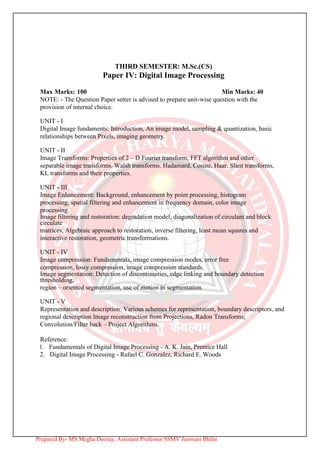
The document provides an overview of a course on digital image processing. It is divided into 5 units that cover topics such as digital image fundamentals, image transforms, image enhancement, image filtering and restoration, image compression, image segmentation, and image representation and description. The course will examine concepts like sampling and quantization, image transforms including Fourier transforms, image enhancement techniques, image compression standards, and image segmentation methods. Students will learn about various image processing schemes and how to reconstruct images from projections using transforms like the Radon transform. The document provides context and outlines the scope of content to be covered in the digital image processing course.
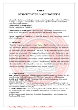
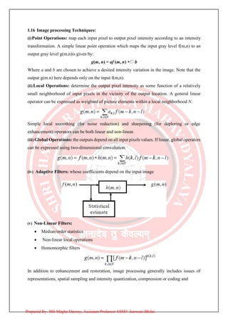
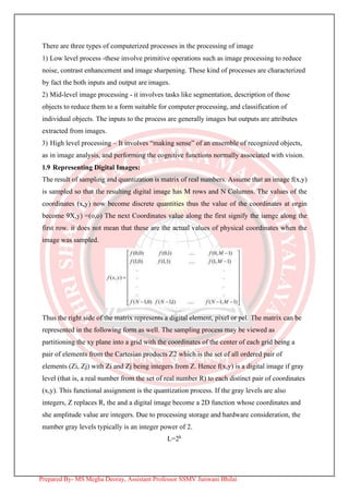
![The functions combine as a product to form f(x,y). We call the intensity of a monochrome
image at any coordinates (x,y) the gray level (l) of the image at that point l= f (x, y.)
L min ≤ l ≤ Lmax
Lmin is to be positive and Lmax must be finite
Lmin = imin rmin
Lmax = imax rmax
The interval [Lmin, Lmax] is called gray scale. Common practice is to shift this interval
numerically to the interval [0, L-l] where l=0 is considered black and l= L-1 is considered white
on the gray scale. All intermediate values are shades of gray of gray varying from black to
white.
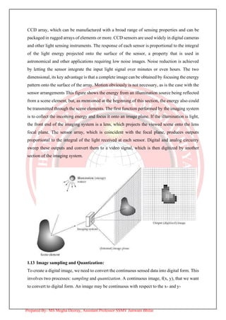
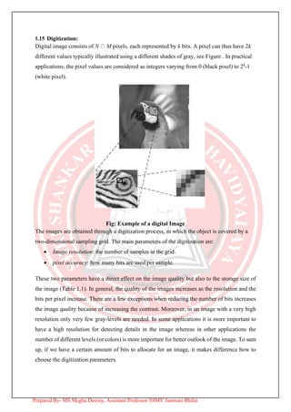
1.7 Image Sampling And Quantization:
To create a digital image, we need to convert the continuous sensed data into digital from. This
involves two processes – sampling and quantization. An image may be continuous with respect
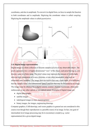
to the x and y coordinates and also in amplitude. To convert it into digital form we have to
sample the function in both coordinates and in amplitudes.
Digitalizing the coordinate values is called sampling.
Digitalizing the amplitude values is called quantization.
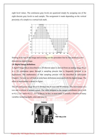
There is a continuous the image along the line segment AB.
To simple this function, we take equally spaced samples along line AB. The location of each
samples is given by a vertical tick back (mark) in the bottom part. The samples are shown as
block squares superimposed on function the set of these discrete locations gives the sampled
function.
In order to form a digital, the gray level values must also be converted (quantized) into
discrete quantities. So we divide the gray level scale into eight discrete levels ranging from
Prepared By- MS Megha Deoray, Assistant Professor SSMV Junwani Bhilai](https://image.slidesharecdn.com/m-201128111308/85/M-sc-iii-sem-digital-image-processing-unit-i-12-320.jpg)
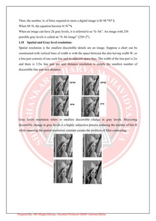
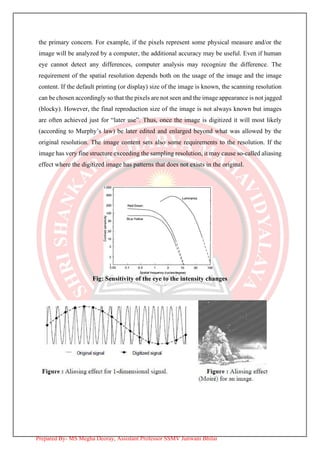
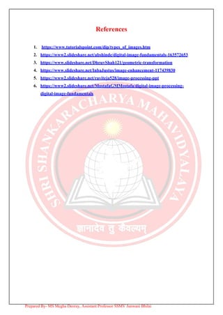
![It is caused by the use of an insufficient number of gray levels on the smooth areas of the digital
image . It is called so because the rides resemble top graphics contours in a map. It is generally
quite visible in image displayed using 16 or less uniformly spaced gray levels.
1.11 Relationship between pixels:
(i) Neighbor of a pixel:
A pixel p at coordinate (x,y) has four horizontal and vertical neighbor whose coordinate can be
given by
(x+1, y) (X-1,y) (X ,y + 1) (X, y-1)
This set of pixel called the 4-neighbours of p is denoted by n4(p) ,Each pixel is a unit distance
from (x,y) and some of the neighbors of P lie outside the digital image of (x,y) is on the border
if the image . The four diagonal neighbor of P have coordinated
(x+1,y+1),(x+1,y+1),(x-1,y+1),(x-1,y-1)
And are deported by nd (p) .these points, together with the 4-neighbours are called 8 –
neighbors of P denoted by ns(p).
(ii) Adjacency:
Let v be the set of gray –level values used to define adjacency, in a binary image, v={1} if
we are reference to adjacency of pixel with value. Three types of adjacency
4- Adjacency – two pixel P and Q with value from V are 4 –adjacency if A is in the set n4(P)
8- Adjacency – two pixel P and Q with value from V are 8 –adjacency if A is in the set n8(P)
M-adjacency –two pixel P and Q with value from V are m – adjacency if
(i) Q is in n4 (p)or
(ii) Q is in nd (q) and the set N4(p) U N4(q) has no pixel whose values are fromV
(iii) Distance measures:
For pixel p,q and z with coordinate (x.y) ,(s,t) and (v,w) respectively D is a distance function
or metric if
D [p.q] ≥ O {D[p.q] = O iff p=q}
D [p.q] = D [p.q] and
D [p.q] ≥ O {D[p.q]+D(q,z)
The Education Distance between p and is defined as
De (p,q) = Iy – t I
The D4 Education Distance between p and is definedas
De (p,q) = Iy – tI
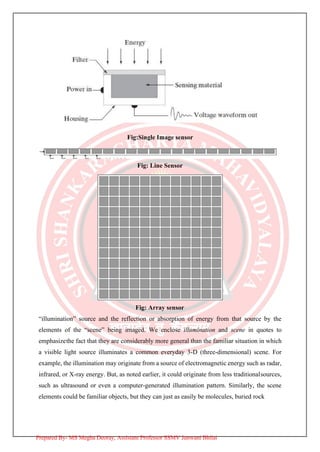
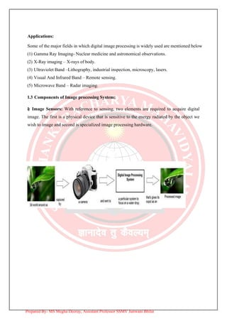
1.12 Image sensing and Acquisition:
The types of images in which we are interested are generated by the combination of an
Prepared By- MS Megha Deoray, Assistant Professor SSMV Junwani Bhilai](https://image.slidesharecdn.com/m-201128111308/85/M-sc-iii-sem-digital-image-processing-unit-i-16-320.jpg)