image processing lectures

1. UNIT-I
INTRODUCTION
Digital image processing is the manipulation of digital images by mean of a computer. It has two main
applications:
 Improvement of pictorial information for human interpretation
 Processing of image data for storage, transmission and representation for autonomous machine
perception.
An image contains descriptive information about the object that it represents. It can be defined
mathematically as a 2-dimensional function or signal f(x,y) where x and y are the spatial coordinates,
and f is called the intensity or gray-level of the image at a point.
A digital image has all the three parameters x, y and f as finite and discrete quantities. It has a finite
number of elements, each of which has a particular location and value. These elements are called
picture elements, image elements, pels or pixels.
Humans are limited to the visual band of the Electromagnetic spectrum (EM). But, imaging machines
cover almost the entire EM spectrum, ranging from gamma to radio waves. Such machines can operate
on images generated by sources including ultrasound, electron microscopy and computer generated
images.
Digital Image Processing encompasses processes whose inputs and outputs are images, and also the
processes that extract attributes from images.
Uses of Digital Image Processing
1. Digital Image Processing techniques are used to enhance the contrast or code the intensity
levels into colors for easier interpretation of X-rays and other images used in industry, medicine,
etc.
2. Geographers use similar techniques to study pollution patterns from aerial and satellite imagery.
3. Image enhancement and restoration procedures are used to process degraded images of
unrecoverable objects or of experimental results that are too expensive to duplicate.
4. In archeology, Digital Image Processing techniques are used to restore blurred pictures that
were the only available records of rare artifacts.
5. Applications of Digital Image Processing for machine perception include automatic character
recognition, industrial machine vision for product assembly and inspection, automatic
processing of fingerprints, screening of X-rays and blood samples, machine processing of aerial
and satellite imagery for weather prediction and environmental assessment.
Fundamental steps in Digital Image Processing
1. Image Acquisition . This step involves acquiring an image in digital form and preprocessing such
as scaling.
2. Image Enhancement – it is the process of manipulating an image so that the result is more
suitable than the original for a specific application. For e.g. filtering, sharpening, smoothing, etc.

2. 3. Image Restoration – these techniques also deal with improving the appearance of an image.
But, as opposed to image enhancement which is based on human subjective preferences
regarding what constitutes a good enhancement result, image restoration is based on
mathematical or probabilistic models of image degradation.
4. Color Image Processing – Color processing in digital domain is used as the basis for extracting
features of interest in an image.
5. Wavelets – they are used to represent images in various degrees of resolution.
6. Image compression – they deal with techniques for reducing the storage required to save an
image, or the bandwidth required to transmit it.
7. Image Segmentation – these procedures partition an image into its constituent parts or objects.
This gives raw pixel data, constituting either the boundary of a region or all the points in the
region itself.
Components of an Image Processing system
1. Image Sensors – two elements are required to acquire a digital image:
a. A physical device that is sensitive to the energy radiated by the object we wish to image.
And,
b. A digitizer for converting the output of the sensor into digital form.
2. Specialized Image Processing Hardware – It must perform primitive operations like arithmetic
and logic operations in parallel on the entire image. Its most distinguishing characteristic is
speed, which the typical computer cannot perform.
3. Computer – This is required for primitive operations and can be a general purpose PC.
4. Software – it consists of specialized modules that perform specific tasks.
5. Mass Storage – short term storage is used during processing, online storage is used for relatively
fast recall, and archival storage is used for infrequent access.
6. Image Displays – These are monitors used to view the result of a processing task.
7. Networking – It is required to transmit images.
ELEMENTS OF VISUAL PERCEPTION
Human intuition and analysis play a central role in the choice of image processing techniques, based on
subjective and visual judgments. So, it is necessary to understand how human and electronic imaging
devices compare in terms of resolution and ability to adapt to changes in illumination.

3. Structure of human eye
The eye is nearly a sphere, with an average diameter of approximately 20mm. three membranes enclose
the eye: the cornea and sclera outer cover, the choroid, and the retina. The innermost membrane of
the eye is the retina, which lines the inside of the wall’s entire posterior portion. When the eye is
properly focused, light from an object outside the eye is imaged on the retina. Discrete light receptors
are distributed over the surface of retina. They are of two types: cones and rods.
Cones are located primarily in the central portion of the retina, called the fovea. They are highly
sensitive to color. Each one is connected to its own nerve end. This helps a person in resolving fine
details. Muscles controlling the eye rotate the eyeball until the image of an object falls on fovea. Cone
vision is called photopic or bright – light vision.
Rods are distributed over the retinal surface. Several rods are connected to a single nerve end. This fact
along with the larger area of distribution reduce the amount of detail discernible by these receptors.
Rods give a general, overall picture of the field of view. They are not involved in color vision and are
sensitive to low levels of illumination. Rod vision is called scotopic or dim – light vision.
Image formation in the eye
In the human eye, the distance between the lens and the retina (imaging region) is fixed, as opposed to
an ordinary photographic camera (where the distance between the lens and film (imaging region) is
varied). The focal length needed to achieve proper focus is obtained by varying the shape of the lens,
with the help of fibers in the ciliary body. The distance between the center of the lens and the retina
along the visual axis is approximately 17mm, and the range of focal lengths is approximately 14mm to
17mm. The retinal image is focused primarily on the region of the fovea. Perception then takes place by

4. the relative excitation of light receptors, which transform radiant energy into electrical impulses that
ultimately are decoded by the brain.
Brightness adaptation and discrimination
The range of light intensity levels to which the human visual system can adapt is enormous – on the
order of 1010
– from scotopic threshold to the glare limit. Subjective brightness (intensity as perceived by
human visual system) is a logarithmic function of the light intensity incident on the eye.
The human visual system cannot operate over the range simultaneously. Rather, it accomplishes this
large variation by changing its overall sensitivity. This is known as brightness adaptation. The total range
of distinct intensity levels the eye can discriminate simultaneously is rather small when compared with
the total adaptation range. For any given set of conditions, the current sensitivity level of the visual
system is called the brightness adaptation level. Brightness discrimination is poor at low levels of
illumination, and it improves significantly as background illumination increases. At low levels of
illumination, vision is carried out by the rods, whereas at high levels, vision is carried out by the cones.

5. Light and Electromagnetic (EM) spectrum.
The EM spectrum ranges from gamma to radio waves. The visible part of the EM spectrum ranges from
violet to red. The part of the spectrum before violet end is called Ultraviolet, and that after red end is
called the Infrared.
Light that is void of color is called monochromatic or achromatic light. Its only attribute is its intensity.
Intensity specifies the amount of light.
Since the intensity of monochromatic light is perceived to vary from black to gray shades and finally to
white, the monochromatic intensity is called Gray level.
The range of measured values of monochromatic light from black to white is called the Gray scale, and
the monochromatic images are called gray scale images.
Chro ati light spa s the EM spe tru fro . μ iolet e d to .79μ red e d .
The quantities that describe the quality of a chromatic light source are
1. Frequency
2. Radiance – it is the amount of energy that flows from the light source and is measured in watts.
3. Luminance – it is the amount of energy that an observer perceives and is measured in lumens.
4. Brightness – it is similar to intensity in achromatic notion, and cannot be measured.

6. Image sensing and acquisition
Images are generated by the combination of an illumination source and the reflection/absorption of
energy from that source by the elements of the scene being imaged. The principal sensor arrangements
used to transform illumination energy into digital images are
1. Single imaging sensor
2. Line sensor
3. Array sensor
The incoming energy is transformed into a voltage by the combination of input electrical power and
sensor material that is responsive to the particular type of energy being detected. The output voltage is
the response of the sensors, and a digital quantity is obtained from each sensor by digitizing its
response.
1. Single imageing sensor This can be a photodiode which is constructed with silicon material and
its output voltage is proportional to the amount of light falling on it. The use of filter in front of
the sensor improves selectivity. For e.g. a green filter results in a stronger sensor output for
green light than other components of the visible spectrum. In order to generate a 2-D image
using a single imaging sensor, there has to be relative displacement in both x- and y- directions
between the sensor and the area to be imaged.
2. Line sensor It consists of an in-line arrangement of sensors in the form of a sensor strip, which
provides imaging elements in one direction. Movement perpendicular to the strip provides
imaging in the other direction. This arrangement is used in most flat-bed scanners. Sensing
devices with 4000 or more in-line sensors are possible. Applications of line sensors include
airborne imaging of geographical areas, medical and industrial imaging to obtain 3-D images of
objects, etc.

7. 3. Array sensor Here the single imaging sensors are arranged in the form of a 2-D array. As the
sensor array is 2-dimensional, a complete image can be obtained by focusing the energy pattern
onto the surface of the array, and hence movement in any direction is not necessary. This
arrangement is found in digital cameras which has CCD sensors packed in arrays of 4000 X 4000
elements or more.
Image Acquisition
The response of each sensor is proportional to the integral of light energy projected onto the surface of
the sensor. The sensor integrates this energy over minutes or hours to reduce the noise.
Acquisition process
 The energy from an illumination source is reflected from the scene element being imaged (or
the energy may be transmitted through the scene element, depending on the nature of its
surface).
 The imaging system collects this reflected/transmitted energy and focuses it onto the image
plane.
 The front end of the imaging system projects the viewed scene onto the lens focal plane.
 The sensor array which is coincidental with the focal plane produces outputs proportional to the
integral of the light received at each sensor, which are then digitized resulting in a digital output
image.
Image Sampling and Quantization
The output of the sensors is a continuous voltage that has to be digitized. This involves two processes –
sampling and quantization.

8. Sampling
It is the process of digitizing the spatial coordinate values. It may be viewed as partitioning the X-Y plane
into a grid of M rows and N columns with the coordinates of the center of each cell in the grid being a
pair from the Cartesian product Ƶ2
. So f(x,y) is a digital image if x,y ϵ Ƶ2
. Each cell is called a picture
element or pixel.
Quantization
It is the process of digitizing the amplitude or intensity values.
Let f(s,t) represent a continuous image function of two continuous variables s and t. to convert it to a
digital image,
1.Sampling – we sample the continuous image into a 2-D array f(x,y) containing M rows and N columns,
where (x,y) are discrete coordinates taking up integer values x= , , ……, M- a d = , ,….., N-1. So
f(0,1) indicates the second sample along the first row. Here, 0 and 1 are not the values of physical
coordinates when the image was sampled.
2. Quantization – the values of the above samples that span a continuous range of intensity values,
must be converted to discrete quantities. This is done by dividing the entire continuous intensity scale
into L discrete intervals, ranging from black to white, where black is represented by a value 0 and white
by L-1. Depending on the proximity of a sample to one of these L levels, the continuous intensity levels
are quantized. In addition to the number of discrete levels used, the accuracy achieved in quantization is
highly dependent on the noise content of the sampled signal.
The digitization process requires that decisions be made regarding values for M, N and L. M and N must
only be positive integers. Due to internal storage and quantizing hardware considerations, the number
of intensity levels typically is an integer power of 2 .i.e., L = 2K
, and the image is referred to as a K-bit
image. For e.g. an image with 256 intensity levels is called an 8-bit image. The number of bits required to
store a digitized k-bit image is b=MNK.

9. Digital Image Fundamentals
1. Dynamic Range - It is the ratio of maximum measurable intensity to the minimum detectable
intensity level in the imaging system. It establishes the lowest and highest intensity levels that
an image can have.
 The upper limit is determined by Saturation. It is the highest value beyond which all
intensity levels are clipped. In an image, the entire saturated area has a high constant
intensity level.
 The lower limit is determined by noise. Especially in the darker regions of an image, the
noise masks the lowest detectable true intensity level.
2. Contrast – It is the difference in intensity between the highest and lowest intensity levels in an
image. For example, a low contrast image would have a dull washed out gray look.
3. Spatial resolution – it is a measure of the smallest detectable detail in an image. It is measured
as line pairs per unit distance, or dots or pixels per unit distance (Dots per Inch or DPI). For
example, newspapers are printed with a resolution of 75DPI, whereas textbooks are printed
with a resolution of 2400 DPI.
4. Intensity Resolution – It is a measure of the smallest detectable change in intensity level. It
refers to the number of bits used to quantize intensity. For example, an image whose intensity is
quantized into 256 levels is said to have 8-bits of intensity resolution.
Basic Relationships between pixels
1. Neighbor of a pixel – we consider the following subset of pixels of an image
L A M
C P D
N B O
Let the position of pixel P be the coordinates (x,y). Then it has two horizontal neighbors and two vertical
neighbors:
Horizontal neighbors : C : (x,y-1)
D : (x,y+1)
Vertical Neighbors : A : (x-1,y)
B : (x+1,y)
These horizontal and vertical neighbors are called the 4-nighbors of P and the set is denoted by
N4(P) = {A, B, C, D} = {(x-1,y), (x+1,y), (x,y-1), (x,y+1)}
If P is on the border of the image, some of the neighbors may not exist.

10. P also has four diagonal neighbors:
L : (x-1,y-1)
M : (x-1,y+1)
N : (x+1,y-1)
O : (x+1,y+1)
This set is denoted by ND(P) ={L, M, N, O}.
All the above are together called the 8-neighbors of P, and are denoted by N8(P). So
N8(P) = N4(P) U ND(P)
2. Adjacency – let V be the set of intensity values used to define adjacency. For example, if we
consider a binary image which has only two intensity values : 0 (representing black) and 1
(representing white), then V can be chosen as V = {1}.
Let V={1} for the following definitions. Consider the following arrangement of pixels (binary image).
0 0 0 0 0
0 0 1(B) 1(C) 0
1(D) 0 1(A) 0 0
1(E) 0 0 0 0
0 1(F) 1(G) 0 0
 4-Adjacency – two pixels p and q with values from set V are said to be 4-adjacent if q is in set
N4(p). For example, in the adjoining figure, A and B are 4-adjacent, since they are 4-neighbors of
each other. But, A and C are not 4-adjaacent.
 8-adjacency - Two pixels p and q with values from set V are 8-adjacent if q is in N8(p).i.e., if p
and q are either horizontal, vertical or diagonal neighbors. For example, in the above figure, (A
and B), (A and C) and (B and C) are 8-adjacent.
 m-adjacency – Two pixels p and q with intensity values from V are m-adjacent if either of the
following two conditions are satisfied:
o q is in N4(p), or
o q is in ND(p), and the set N4(p) N4(q) has no pixels with values from V.
For example, in the above figure, (A and B), (B and C), (D and E) and (F and G) are m-adjacent
since they satisfy the first condition. (E and F) are also m-adjacent since they satisfy the second
condition, although they violate the first condition. (A and C) are not m-adjacent since they
violate both conditions.
3. Path - a path from pixel p with coordinates (x,y) to pixel q with coordinates (s,t) is a sequence of
distinct pixels with coordinates (x0, y0), (x1, y1 , … n, yn) where pixels (xi , yi) and (xi-1 , yi-1) are

11. adja e t for ≤ i ≤ , a d here 0, y0) =(x,y) and (xn , yn) = (s,t).
 Here, n is the length of the path.
 If (x0 , y0) and (xn , yn) are the same, then the path is a closed path.
 Depending on the type of adjacency, we can have 4-path, 8-path or m-path.
0 1(A) 1(B)
0 1(C) 0
0 0 1(D)
For example, in the above arrangement of pixels, the paths are as follows:
4-path : B A C
8-paths: (i) B A C, (ii) B A C D, (iii)B C D
m-path: B A C D
4. Connectivity – let S represent a subset of pixels in an image. Then, two pixels p and q are said to
be connected in S, if there exists a path between them consisting entirely of pixels in S. For
example, in the previous figure, if all the 9 pixels form the subset S, then B and C (or B and D in
case of 8 and m-paths) are said to be connected to each other. On the other hand, if S consists
of pixels of rightmost column, then B and D are not connected to each other.
 For any pixel p in S, the set of pixels that are connected to it in S is called a connected
component of S. for example, if all the 9 pixels in the above figure form S, the pixels A, B, C and
D form a connected component.
 If the subset S has only one connected component, then the set S is called a connected set. For
example,
(i) The following is a connected set
0 0 0 0 0
0 0 1 1 0
0 0 1 0 0
0 0 0 1 0
0 0 0 0 0
(ii) The following subset is not a connected set, since it has two connected components.
0 0 0 0 0
0 0 1 1 0
0 0 1 0 0
0 0 0 1 0
0 0 0 0 0
0 0 1 1 0
0 0 0 1 0
0 0 0 0 0
5. Region – let R be a subset of pixels of an image. R is called a region of the image, if R is a
connected set.

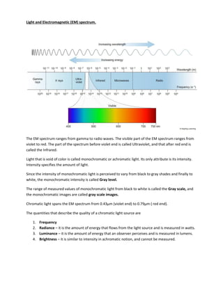
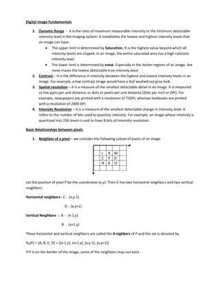
12.  Two regions Ri and Rj are said to be adjacent if their union forms a connected set.
Regions that are not adjacent are said to be disjoint. We consider 4 and 8-adjacency
only when referring to regions. For example, considering two regions Ri and Rj as
follows:
1 1 1
1 0 1
0 1(A) 0
0 0 1(B)
1 1 1
1 1 1
Pixels A and B are 8-adjacent but not 4-adjacent. Union of Ri and Rj will form a connected set if 8-
adjacency is used, and then Ri and Rj will be adjacent regions. If 4-adjacency is used, they will be
disjoint regions.
6. Boundary – let an image contain K disjoint regions. Let RU denote the pixels in the connected
components of the union of all these K regions, and let RU
C
denote its complement. Then RU is
called the foreground and RU
C
is called the background of the image. The inner
border/boundary of a region R is the set of pixels in the region that have atleast one
background neighbor (adjacency must be specified).
7. Distance Measures – consider pixels p and q with coordinates (x,y) and (s,t) respectively.
 Euclidean distance – it is defined as 𝑒 , = √[ − + − ]. All the pixels
that have Euclidean distance less than or equal to a value r from pixel p(x,y) are
contained in a disk of radius r centered at (x,y).
 D4 distance (City-block distance) – it is defined as 4 , = | − | + | − |. All the
pixels having D4 distance less than or equal to a value r are contained in a diamond
centered at (x,y). Also, all the pixels with D4 =1 are the 4-neighbors of (x,y).
 D8 distance ( Chessboard distance) – it is defined as 8 , = | − | , | − | .
All the pixels with D8 distance less than or equal to some value r from (x,y) are contained
in a square centered at (x,y). All pixels with D8 =1 are the 8-neigbors of (x,y).
 De , D4 and D8 distances are independent of any paths that may exist between p and q.
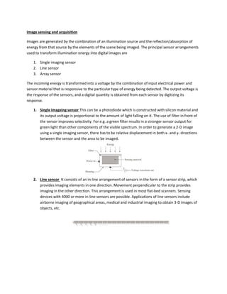
 Dm distance – it is defined as the shortest m-path between p and q. So, the Dm distance
between two pixels will depend on the values of the pixels along the path, as well as on
the values of their neighbors. For example, consider the following subset of pixels
P8 P3 P4
P1 P2 P6
P P5 P7
Ri
Rj

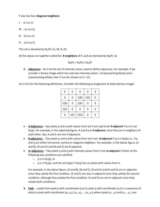
13. For adjacency, let V={1}. Let P, P2 and P4 =1
i) If P1, P3, P5, P6, P7, and P8 = 0. Then the Dm distance between P and P4 is 2
(only one m-path exists: P – P2 – P4)
0 0 1
0 1 0
1 0 0
ii) If P, P1 , P2 and P4 =1, and rest are zero, then the Dm distance is 3 (P – P1 –
P2 – P4)
0 0 1
1 1 0
1 0 0
Mathematical Tools used in Digital Image Processing
1. Array versus Matrix operations – Array operations in images are carried out on a pixel – by –
pixel basis. For example, raising an image to a power means that each individual pixel is raised
to that power. There are also situations in which operations between images are carried out
using matrix theory.
2. Linear versus Nonlinear operations – considering a general operator H that when applied on an
input image f(x,y) gives an output image g(x,y) .i.e.,
[ , ] = ,
Then, H is said to be a linear operator if
[ , + , ] = , + ,
Where, a and b are arbitrary constants. f1(x,y) and f2(x,y) are input images, and g1(x,y) and
g2(x,y) are the corresponding output images.
That is, if H satisfies the properties of additivity and homogeneity, then it is a linear operator.
3. Arithmetic operations – these operations are array operations and are denoted by
S(x,y) = f(x,y) + g(x,y)
D(x,y) = f(x,y) – g(x,y)
P(x,y) = f(x,y) * g(x,y)
V(x,y) = f(x,y) ÷ g(x,y)
These operations are performed between corresponding pixel pairs i f a d g for = , , , …
M- a d = , , , …, N-1, where all the images are of size M X N.
For example,
 if we consider a set of K noisy images of a particular scene {gi(x,y)}, then, in order to obtain an
image with less noise, averaging operation can be done as follows:
̅ , =
𝐾
∑ ,
𝐾
=
This averaging operation can be used in the field of astronomy where imaging under very low
light levels frequently causes sensor noise to render single images virtually useless for analysis.
 Image Subtraction – this operation can be used to find small minute differences between
images that are indistinguishable to the naked eye.

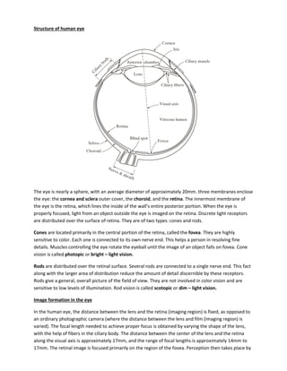
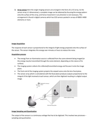
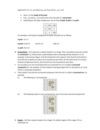
14.  Image Multiplication – this operation can be used in masking where some regions of interest
need to be extracted from a given image. The process consists of multiplying a given image with
a mask image that has 1s in the region of interest and 0s elsewhere.
 In practice, for an n-bit image, the intensities are in the range [0 , K] where K = 2n
– 1. When
arithmetic operations are performed on an image, the intensities may go out of this range. For
example, image subtraction may lead to images with intensities in the range [ - 255 , 255]. In
order to bring this to the original range [0, K], the following two operations can be performed. If
f(x,y) is the result of the arithmetic operation, then
o We perform , = , − [ , ]. This creates an image whose minimum
value is zero.
o Then, we perform
, = 𝐾 [
,
[ , ]
]
This results in an image fS (x,y) whose intensities are in the range [ 0 , K ].
 While performing image division, a small number must be added to the pixels of divisor image to
avoid division by zero.
4. Set Operations – for gray scale images, set operations are array operations. The union and
intersection operations between two images are defined as the maximum and minimum of
corresponding pixel pairs respectively. The complement operation on an image is defined as the
pairwise differences between a constant and the intensity of every pixel in the image.
Let set A represent a gray scale image whose elements are the triplets (x, y, z) where (x,y) is the
location of the pixel and z is its intensity. Then,
Union :
= {max , | ∈ , ∈ }
Intersection:
= {min , | ∈ , ∈ }
Complement:
= { , , 𝐾 − | , , ∈ }
5. Logical Operations – when dealing with binary images, the 1 – valued pixels can be thought of
as foreground and 0 – valued pixels as background. Now, considering two regions A and B
composed of foreground pixels,
The OR operation of these two sets is the set of coordinates belonging either to A or to B or to
both.
The AND operation is the set of elements that are common to both A and B.
The NOT operation on set A is the set of elements not in A.
The logical operations are performed on two regions of same image, which can be irregular and
of different sizes.
The set operations involve complete images.

15. IMAGE TRANSFORMS
Need for Transforms
Transform is the process of representing data in a different domain that is different from the raw
domain. This is done because some image processing tasks are best formulated by transforming the
input images, carrying the specified task in the transform domain, and applying the inverse transform to
return back to spatial domain. If ̅ is an N – by – 1 vector and ̅ is an N – by – N matrix, then ̅ = ̅ ̅ is a
linear transformation of vector ̅. It is called forward transformation. ̅ is called the kernel matrix. The
inverse transformation is given by ̅ = ̅−
̅. To make the transformation invertible, ̅ must be non –
singular.
The inner product of any row of ̅ with itself is 1, and with any other row it is 0. So, the rows of ̅ are a
set of orthonormal vectors, and form an orthonormal basis for the N – dimensional vector space of all N
– by – 1 vectors.
The forward transformation is the process of analysis, breaking the signal vector down into its
elemental components.
The inverse transformation is the process of synthesis, reassembling the original vector from its
components.
The discrete image transforms are classified into three categories:
1. Sinusoidal Transforms – they use sinusoidal basis functions. For example, Discrete Sine
Transform (DST), Discrete Cosine Transform (DCT), Discrete Fourier Transform (DFT), etc.
2. Rectangular wave Transforms – They use basis functions that are variations of a square wave.
They are fast to compute since many of the multiplications become trivial. For example, Haar,
Walsh, Hadamard transforms, etc.
3. Eigenvector based transforms – they use basis functions that are derived from eigenanalysis.
For example, KL transform, Singular Value Decomposition, etc.
I. Sinusoidal Transforms
A. Discrete Fourier Transform
Fourier Transform is an important image processing tool which is used to decompose an image
into its frequency components. It serves as an important tool in image analysis, image filtering,
image reconstruction, image compression, etc. the 2-dimensional Fourier Transform of an image
f (s,t) is given by
, = ∫ ∫ , − +
∞
−∞
∞
−∞
Where are called the spatial frequencies.
For digital images, we consider the 2 – D DFT. This DFT is the sampled version of the previous
equation. So, the 2 – D DFT does not contain all the frequencies forming the image. The image in
the spatial and frequency domain are of the same size.
if f (x,y) is an M X N digital image, then its 2-D DFT F (u,v) is given by

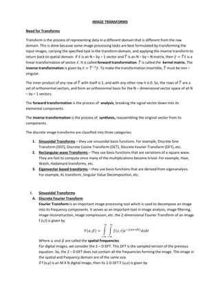
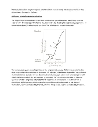
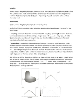
16. F u, v = ∑ ∑ f x, y e
−j π
e
−j π
−
=
−
=
= , , , … , −
= , , , … , −
Each point in the DFT gives the value of the image at a particular frequency. For example, F(0 , 0)
represents the DC – component of the image and gives the average brightness of the image. Similarly,
F(N-1 , N-1) represents the highest frequency (sharp edges).
Since F(u , v) is seperable, it can be written as
, = ∑ 𝑃 , − 𝜋 /
−
=
where
𝑃 , = ∑ , − 𝜋 /
−
=
So, the 2 – D DFT of an image can be obtained by first applying the second equation above on the image,
which is applying a 1 – Dimensional N – point DFT on the rows of the image to get an intermediate
image. Then the first equation above is applied on the intermediate image, which is applying 1- D DFT on
the columns of the intermediate image.
Applying a 1 – D DFT has N2
complexity. This can be reduced to log using the Fast Fourier
Transform.
The 2-D inverse DFT is given by
f x, y =
MN
[∑ ∑ F u, v e
j π
e
j π
−
=
−
=
]
= , , , … , −
= , , , … , −
The DFT pair can also be expressed in the matrix form. If ̅ is the image matrix, ̅ is the spectrum matrix,
and ̅ is the kernel matrix, then the DFT or spectrum can be obtained by
̅ = ̅ ̅ ̅ where
̅ = [
, , , −
, , ⋱
− , −
]
Where
, =
√
− 𝜋
All the matrices are of size N X N.

17. Properties of 2-D DFT
1. Relation between spatial intervals and frequency intervals
In 1-dimension, if f(n) consists of M sa ples of a fu tio f t take ΔT u its apart sa pli g
period), then
= = ∆
Then, its 1-D Discrete Fourier Transform is given by
= ∑ − 𝜋 /
And its Discrete Time Fourier Transform (DTFT) is given by
( 𝜔
) = ∑ − 𝜔 ∆
= ∑ − 𝜋 ∆
u =cyclic frequency
to o ert DTFT to DFT, e dis retize i ω at 𝜔 =
𝜋
∆
or at =
∆
∵ 𝜔 = 𝜋
from above, it can be found that the spacing between the frequencies is
∆ =
∆
In 2-D case, f(t,z) is a continuous image which is sampled to obtain digital image f(x,y) consisting of M
samples in t-direction and N samples in z-dire tio . Let ΔT a d ΔZ e the spatial i ter als i t a d z-
directions. Then, the frequency intervals are given by
∆ =
∆
, ∆ =
∆
The frequency spacing is inversely proportional to both the spatial spacing and to the number of
samples in that direction.
2. Translation property
This property states that if f(x, y) has a 2-D DFT given by F (u, v), then
,
𝜋 0 + 0 − 𝐹
↔ − , −
And
− , −
− 𝐹
↔ ,
− 𝜋 0 + 0
i.e., a translation or shift in one domain results in a phase shift in other domain.
If u0 = M/2 and v0 = N/2, then from above relation,
, − +
− 𝐹
↔ − , −
i.e., the spectrum of an image can be shifted to the center of the grid, by multiplying the
intensity of every pixel in the image in spatial domain by − +
(where (x,y) is the location of the
pixel).

18. 3. Rotation Property
This property can be obtained by expressing the independent variables in polar form instead of
Cartesian coordinates, as follows:
Spatial coordinates: =r osθ , =rsi θ
Frequency variables: u=ω osφ , = ωsi φ
Image in spatial domain in polar form : f r, θ
Image in transform domain (DFT of the image) in polar form : F ω , φ)
Then, it can be shown that the 2-D DFT relation can be expressed as
F ω, ∅ = ∑ ∑ f r, θ e
−j π
ω co θ−∅
−
=
−
=
No , a ordi g to rotatio propert , if the i age is rotated a a gle θ0, its DFT (in polar
form) is given by
, 𝜃 + 𝜃
− 𝐹
↔ 𝜔, ∅ + 𝜃
4. Periodicity
This property states that the 2-D DFT is periodic in both variables u and v, with period M or N or
both. i.e.,
+ 𝐾 , = , + 𝐾 = + 𝐾 , + 𝐾 = ,
5. Symmetry Properties
Any image f(x,y) can be expressed as a sum of an even and an odd function as follows
, = 𝑒 , + ,
Where
𝑒 , ≜
, + − , −
, ≜
, − − , −
Even function is a symmetric function .i.e., 𝑒 , = 𝑒 − , −
And, odd function is antisymmetric .i.e., , = − − , −
Since all the indices in the DFT or IDFT are positive, the symmetry or antisymmetry is defined
about the center point of the sequence. The indices to the right of center are considered
positive, and those to the left are considered negative. So, the even and odd functions are
redefined as follows:
Even function : 𝑒 , = 𝑒 − , −
And, odd function : , = − − , −

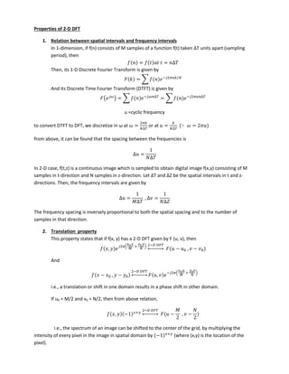
19. B. 2-D Discrete Sine Transform
For an N X N image g ( i , k ), its 2-D Discrete Sine Transform, GS (m,n) is given by
, =
+
∑ ∑ , sin [
𝜋 + +
+
] sin [
𝜋 + +
+
]
−
=
−
=
And, the inverse Discrete Sine Transform is given by
, =
+
∑ ∑ , sin[
𝜋 + +
+
] sin [
𝜋 + +
+
]
−
=
−
=
In matrix notation, the kernel matrix ̅ has elements of ith
row and kth
column given by
, = √
+
[
𝜋 + +
+
]
Discrete Sine Transform is most conveniently computed for matrix sizes N=2P
– 1 where P is an
integer.
C. 2-D Discrete Cosine Transform
For an N X N image g ( i , k ), its 2-D Discrete Cosine Transform, GC (m,n) is given by
, = ∑ ∑ , cos[
𝜋 +
] cos[
𝜋 +
]
−
=
−
=
And, the inverse Discrete Cosine Transform is given by
, = ∑ ∑ , cos [
𝜋 +
] cos [
𝜋 +
]
−
=
−
=
Where
= √ , = √ , ≤ ≤
In matrix notation, the kernel matrix ̅ has elements of ith
row and mth
column given by
, = [
𝜋 +
]
II. Rectangular Wave Based Transforms
A. Haar Transform
Haar functions are recursively defined by the equations
≡ ≤ <
≡ {
≤ < /
− ≤ <
𝑝+ ≡
{
√ ≤ <
+ .
−√
+ .
≤ <
+
ℎ

20. Where
= , , ,
= , , , −
In order to apply Haar transform on an image, it is required to create the image kernel matrix.
This matrix is created from the above Haar function as follows:
 First, the independent variable t is scaled by the size of the matrix.
 Then, the values of the function at integer values of t are considered.
 These HK(t) values are then written in matrix form where K is the row number and the integer
alues of t are the olu u ers. i.e., K= , , … , N- , a d t = , , … , N-1.
 Finally, the matrix is normalized by multiplying with
√
to obtain orthonormal basis vectors.
B. Walsh Transform
The Walsh kernel matrix is also formed in the same way as the Haar kernel matrix, where the Walsh
functions are given by
+ = −
+
{ + − +
− }
Where
=
= , , ,
= {
≤ <
, ℎ
is the highest integer less than .
C. Hadamard Transform
It exists for matrix sizes of N = 2n
, where n is an integer. For a 2 X 2 image, the transform matrix is
given by
= [
−
]
And for an N X N image for N >2, the transform matrix is obtained recursively as follows
= [
/ /
/ − /
]
D. Slant Transform
For a 2 X 2 image, the transform matrix is given by
= [
−
]
For an N X N image for N > 2, the transform matrix can be obtained as follows

21. =
[
𝟎
̅
−
𝟎
̅
𝟎
̅ 𝑰
̅ 𝟎
̅ 𝑰
̅
−
𝟎
̅
−
𝟎
̅
𝟎
̅ 𝑰
̅ 𝟎
̅ − 𝑰
̅ ]
[
𝑺𝑵/𝟐
̅̅̅̅̅̅ 𝟎
̅
𝟎
̅ 𝑺𝑵/𝟐
̅̅̅̅̅̅
]
𝑰
̅ 𝟎
̅ are the Identity and zero matrices respectively of order −
And,
= √
−
= √
−
−
III. Eigenvector based Transforms
A. Singular Value Decomposition (SVD Transform)
Any N X N matrix ̅ can be expressed as
̅ = ̅𝑃
̅ ̅
Here, 𝑃
̅ is the N X N diagonal matrix, where the diagonal elements are the singular values of ̅. Columns
of ̅ and ̅ are the eigenvectors of ̅ ̅ and ̅ ̅ respectively. The above relation is the inverse
transform. The forward SVD transform is given by
𝑃
̅ = ̅ ̅ ̅
If ̅ is a symmetric matrix, ̅ = ̅ . and, in this SVD transform, the kernel matrices ̅ and ̅
depend on the image ̅ being transformed.
B. KL Transform
In order to obtain the KL transform of an image, the rows corresponding to the image are
arranged in the form of column vectors.
 Let ̅ , ̅ , … e the olu e tors orrespo di g to the st
, 2nd
, 3rd
, … ro s of a i age.
 Then the image is represented as ̅ = [
̅
̅ ]. The mean vector of this is obtained. i.e., ̅ = [ ̅].
 Now, the covariance matrix is given by ̅ = [ ̅ − ̅ ̅ − ̅ ] , here E[•] is the
expectation / mean. Simplifying this, we obtain, ̅ = [ ̅ ̅ ] − [ ̅ ̅ ]
 A matrix ̅ is formed by arranging the eigenvectors of ̅ as the rows of ̅ .
 The average ( ) of each column is subtracted from each element of ̅.
 Then, each vector ̅ is transformed by using the following expression
̅ = ̅ ̅ −

22.  This transformation results in a transformed vector ̅ , whose covariance matrix ̅ is a diagonal
matrix, which implies that each pixel in the transformed vector is uncorrelated with every other
pixel.
FACULTY
ECE-1 & 2: B.V.S.RENUKA DEVI