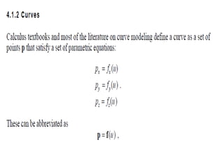
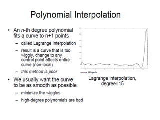
Download to read offline

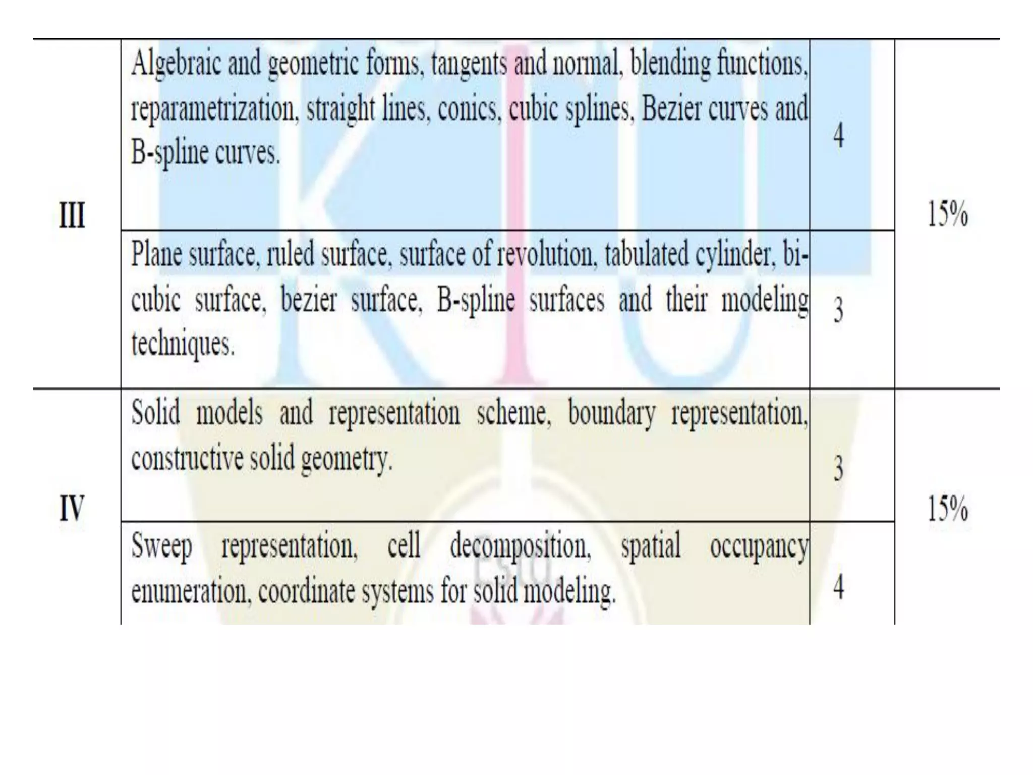
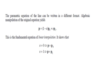
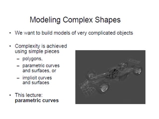
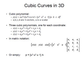
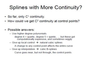
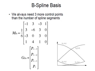
![Composite Bezier Surface
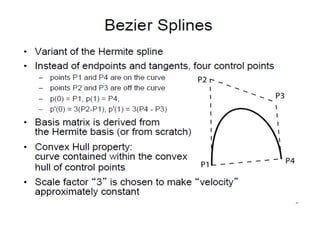
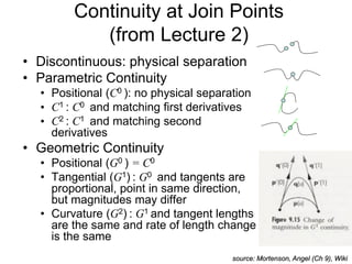
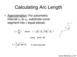
• Bezier surface patches can
provide G1 continuity at patch
boundary curves.
• For common boundary curve
defined by control points p14,
p24, p34, p44, need collinearity
of:
• Two adjacent patches are Cr
across their common boundary
iff all rows of control net
vertices are interpretable as
polygons of Cr piecewise
Bezier curves.
source: Mortenson, Farin
]
4
:
1
[
},
,
,
{ 5
,
4
,
3
,
i
i
i
i p
p
p
•Cubic B-splines can provide C2 continuity at surface patch boundary curves.](https://image.slidesharecdn.com/module3-221008151041-19008608/85/Module-3-pdf-59-320.jpg)
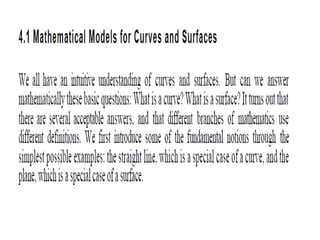
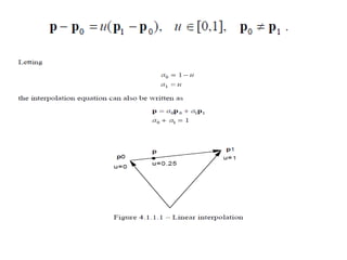
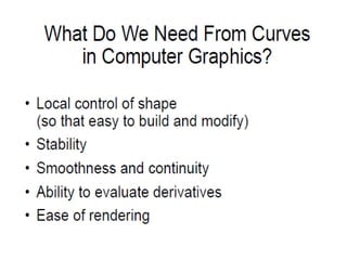
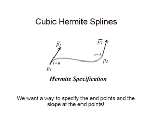
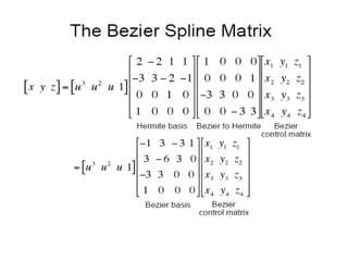
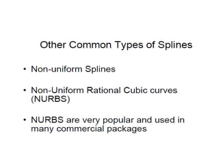
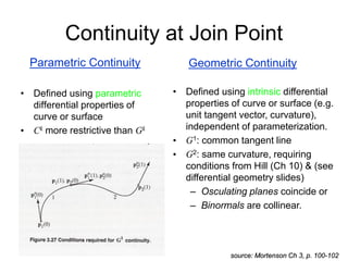
![Continuity within a
(Single) Curve Segment
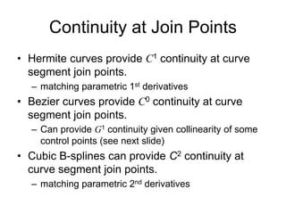
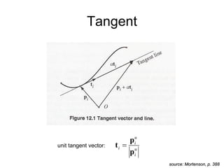
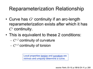
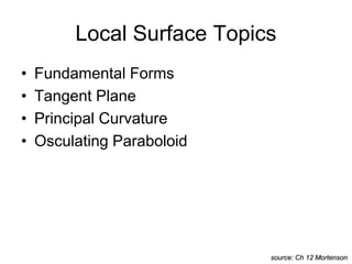
• Parametric Ck Continuity:
– Refers to the parametric curve representation and parametric
derivatives
– Smoothness of motion along the parametric curve
– “A curve P(t) has kth-order parametric continuity everywhere in the
t-interval [a,b] if all derivatives of the curve, up to the kth, exist and
are continuous at all points inside [a,b].”
– A curve with continuous parametric velocity and acceleration has
2nd-order parametric continuity.
cos
)
( b
Ke
x
source: Hill, Ch 10
sin
)
( b
Ke
y
)
)(
)(
(cos
)
sin
)(
(
)
(
'
b
b
b
be
Ke
Ke
x
)
)(
)(
(sin
)
)(cos
(
)
(
'
b
b
b
be
Ke
Ke
y
apply product rule
1st derivatives of parametric expression are
continuous, so spiral has 1st-order (C1) parametric
continuity.
Note that Ck continuity implies Ci
continuity for i < k.
Example](https://image.slidesharecdn.com/module3-221008151041-19008608/85/Module-3-pdf-60-320.jpg)
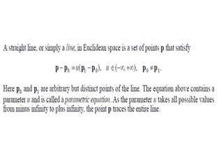
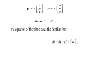
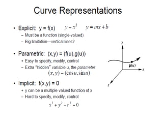
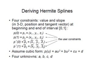
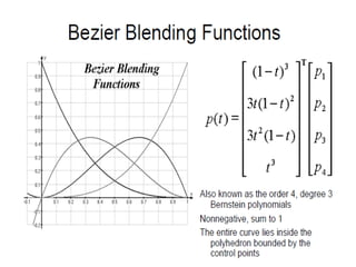
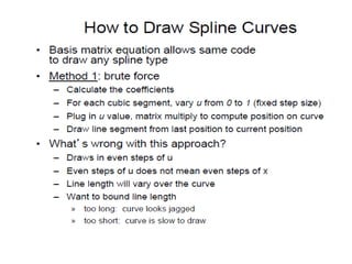
![Continuity within a
(Single) Curve Segment (continued)
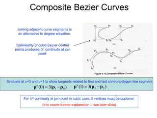
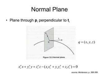
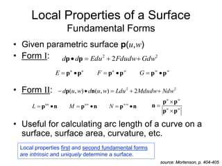
• Geometric Gk Continuity in interval [a,b] (assume P is curve):
– “Geometric continuity requires that various derivative vectors have
a continuous direction even though they might have discontinuity in
speed.”
– G0 = C0
– G1: P’(c-) = k P’(c+) for some constant k for every c in [a,b] .
• Velocity vector may jump in size, but its direction is continuous.
– G2: P’(c-) = k P’(c+) for some constant k and P’’(c-) = m
P’’(c+) for some constants k and m for every c in [a,b] .
• Both 1st and 2nd derivative directions are continuous.
Note that, for these definitions, Gk continuity implies Gi continuity for i < k.
source: Hill, Ch 10
These definitions suffice for that textbook’s treatment, but there is more to the story…](https://image.slidesharecdn.com/module3-221008151041-19008608/85/Module-3-pdf-61-320.jpg)
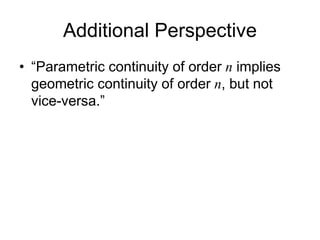
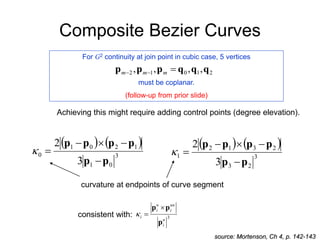
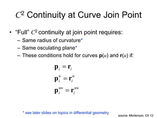
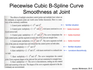
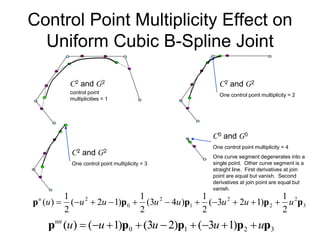
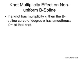
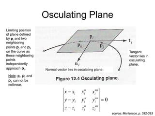
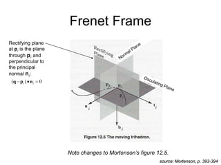
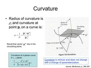
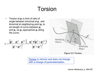
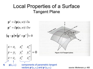
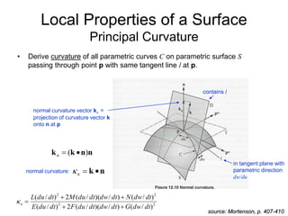
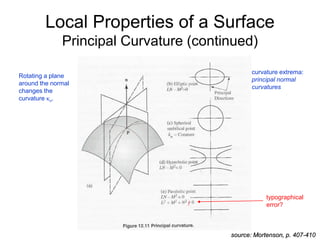
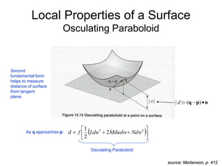
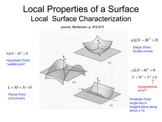

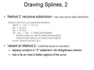
The document discusses various types of continuity for curves and surfaces at join points. It defines positional (C0), tangent (G1), and curvature (G2) continuity geometrically and parametrically. Parametric continuity implies the same level of geometric continuity but not vice versa. Cubic Bézier curves can provide G1 continuity, Hermite curves provide C1 continuity, and cubic B-splines can provide C2 continuity. Knot multiplicity affects continuity for B-splines. The document also introduces concepts from differential geometry related to continuity, such as curvature and torsion.