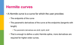
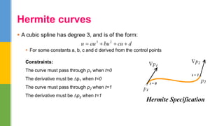
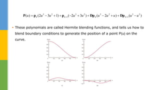
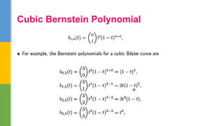
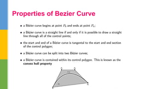
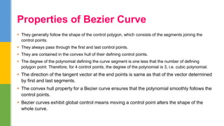
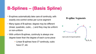
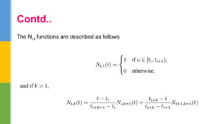
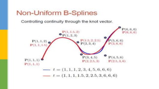
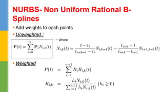
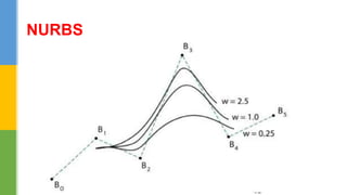
HERMITE CURVES & BEIZER
CURVES
 A Hermite curve is a curve for which the user provides:
 The endpoints of the curve
 The parametric derivatives of the curve at the endpoints (tangents with
length)
 The parametric derivatives are dx/dt, dy/dt, dz/dt
 That is enough to define a cubic Hermite spline, more derivatives are
required for higher order curves.
Hermite curves
 A cubic spline has degree 3, and is of the form:
 For some constants a, b, c and d derived from the control points
Hermite curves
Constraints:
The curve must pass through p1 when t=0
The derivative must be ∆p1 when t=0
The curve must pass through p2 when t=1
The derivative must be ∆p2 when t=1
dcubuauu  23
 Control point positions and first derivatives are given as constraints for each end-point.
 













d
c
b
a
P 1)( 23
uuuu  













d
c
b
a
P 0123)( 2
uuu








































d
c
b
a
Dp
Dp
p
p
0123
0100
1111
1000
1
1
k
k
k
k
→






















































































1
1
1
1
1
1
1
0001
0100
1233
1122
0123
0100
1111
1000
k
k
k
k
H
k
k
k
k
k
k
k
k
Dp
Dp
p
p
M
Dp
Dp
p
p
Dp
Dp
p
p
d
c
b
a
End point constraints for each segment is given as:
,)1(,)0(,)1(,)0( 11   kkkk DpPDpPpPpP
 These polynomials are called Hermite blending functions, and tells us how to
blend boundary conditions to generate the position of a point P(u) on the
curve.
)()2()32()132()( 23
1
2323
1
23
uuuuuuuuuu kkkk   DpDpppP
 More degrees of freedom
 Directly transformable
 Dimension independent
 No infinite slope problems
 Separates dependent and independent variables
 Inherently bounded
 Easy to express in vector and matrix form
 Common form for many curves and surfaces
Advantages of parametric forms
Bezier Curve
Bezier Curve – Parametric Equation
Quadratic Bezier Curve - Derivation
Contd..
De Casteljau’s Algorithm
Cubic Bezier Curve
Design of n Bezier Curve
Binomial Coefficient
Cubic Bernstein Polynomial
Behaviour of Bernstein Polynomial
Matrix Form – Bezier Curves
Properties of Bezier Curve
 They generally follow the shape of the control polygon, which consists of the segments joining the
control points.
 They always pass through the first and last control points.
 They are contained in the convex hull of their defining control points.
 The degree of the polynomial defining the curve segment is one less that the number of defining
polygon point. Therefore, for 4 control points, the degree of the polynomial is 3, i.e. cubic polynomial.
 The direction of the tangent vector at the end points is same as that of the vector determined
by first and last segments.
 The convex hull property for a Bezier curve ensures that the polynomial smoothly follows the
control points.
 Bezier curves exhibit global control means moving a control point alters the shape of the
whole curve.
Properties of Bezier Curve
Examples
 B-splines automatically take care of continuity, with
exactly one control vertex per curve segment
 Many types of B-splines: degree may be different
(linear, quadratic, cubic,…) and they may be uniform
or non-uniform
 With uniform B-splines, continuity is always one
degree lower than the degree of each curve piece
 Linear B-splines have C0 continuity, cubic
have C2, etc
B-Splines – (Basis Spline)
B-Spline – Analytical Definition
normally called the “Knot Sequence”.
Contd..
The Ni,k functions are described as follows
 The sum of the B-spline basis functions for any parameter value is 1.
 Each basis function is positive or zero for all parameter values.
 Each basis function has precisely one maximum value, except for k=1.
 The maximum order of the curve is equal to the number of vertices of
defining polygon.
 The degree of B-spline polynomial is independent on the number of vertices
of defining polygon.
 B-spline allows the local control over the curve surface because each vertex
affects the shape of a curve only over a range of parameter values where its
associated basis function is nonzero.
Properties of B-Spline Curves
Bezier Curve vs B-Spline - Control
The choice of a knot vector directly influences the resulting curve.
Types of Knot vectors
 Uniform (periodic)
 Open-Uniform
 Non-Uniform
Knot Vectors
 Open curves expect that do not passes through the first and last
control points and therefore are not tangent to the first and last
segment of the control polygon.
 Closed curves where the first and last control points curve
connected. Closed curves with the first and last control point
being the same (coincident ).
Open and closed B-spline curves
 When the spacing between knot values is constant, the
resulting curve is called a uniform B-spline.
 The spacing between knot values is not constant and hence
,any values and intervals can be specified for the knot vector
the curve is called a non uniform B-spline .
 Different intervals which can be used to adjust spline shapes .
Uniform and non uniform B-spline curves
 Rational curves is defined as ratio of two polynomials.
 Non rational curves is defined by one polynomials.
 The most widely used rational curves are non uniform rational
B-splines (NURBS)
 NURBS is capable of representing in a single form non –rational
B-splines and Bezier curves as well as linear and quadratic
analytic curves.
Rational Curves
 Add weights to each points
 Unweighted :
 Where
 Weighted
NURBS- Non Uniform Rational B-
Splines
NURBS
 Rational curve can handle both analytical and synthetic curves.
 Rational curve represents a point with homogenous coordinate
system where a 3D coordinate system is expressed as (wi x, wi
y ,wi z,wi).
 Using same control points with different weights ,different
curves can be generated.
 The weight associated with each control point can affect the
curve locally and the curve is pulled towards the control point
with increases valued of its weight wi.
Characteristics of Rational curves
THANK YOU

Hermit curves & beizer curves

  • 1.
    HERMITE CURVES &BEIZER CURVES
  • 2.
     A Hermitecurve is a curve for which the user provides:  The endpoints of the curve  The parametric derivatives of the curve at the endpoints (tangents with length)  The parametric derivatives are dx/dt, dy/dt, dz/dt  That is enough to define a cubic Hermite spline, more derivatives are required for higher order curves. Hermite curves
  • 3.
     A cubicspline has degree 3, and is of the form:  For some constants a, b, c and d derived from the control points Hermite curves Constraints: The curve must pass through p1 when t=0 The derivative must be ∆p1 when t=0 The curve must pass through p2 when t=1 The derivative must be ∆p2 when t=1 dcubuauu  23
  • 4.
     Control pointpositions and first derivatives are given as constraints for each end-point.                d c b a P 1)( 23 uuuu                d c b a P 0123)( 2 uuu                                         d c b a Dp Dp p p 0123 0100 1111 1000 1 1 k k k k →                                                                                       1 1 1 1 1 1 1 0001 0100 1233 1122 0123 0100 1111 1000 k k k k H k k k k k k k k Dp Dp p p M Dp Dp p p Dp Dp p p d c b a End point constraints for each segment is given as: ,)1(,)0(,)1(,)0( 11   kkkk DpPDpPpPpP
  • 5.
     These polynomialsare called Hermite blending functions, and tells us how to blend boundary conditions to generate the position of a point P(u) on the curve. )()2()32()132()( 23 1 2323 1 23 uuuuuuuuuu kkkk   DpDpppP
  • 6.
     More degreesof freedom  Directly transformable  Dimension independent  No infinite slope problems  Separates dependent and independent variables  Inherently bounded  Easy to express in vector and matrix form  Common form for many curves and surfaces Advantages of parametric forms
  • 7.
  • 8.
    Bezier Curve –Parametric Equation
  • 9.
  • 10.
  • 11.
  • 12.
  • 13.
    Design of nBezier Curve
  • 14.
  • 15.
  • 16.
  • 17.
    Matrix Form –Bezier Curves
  • 18.
  • 19.
     They generallyfollow the shape of the control polygon, which consists of the segments joining the control points.  They always pass through the first and last control points.  They are contained in the convex hull of their defining control points.  The degree of the polynomial defining the curve segment is one less that the number of defining polygon point. Therefore, for 4 control points, the degree of the polynomial is 3, i.e. cubic polynomial.  The direction of the tangent vector at the end points is same as that of the vector determined by first and last segments.  The convex hull property for a Bezier curve ensures that the polynomial smoothly follows the control points.  Bezier curves exhibit global control means moving a control point alters the shape of the whole curve. Properties of Bezier Curve
  • 20.
  • 21.
     B-splines automaticallytake care of continuity, with exactly one control vertex per curve segment  Many types of B-splines: degree may be different (linear, quadratic, cubic,…) and they may be uniform or non-uniform  With uniform B-splines, continuity is always one degree lower than the degree of each curve piece  Linear B-splines have C0 continuity, cubic have C2, etc B-Splines – (Basis Spline)
  • 23.
    B-Spline – AnalyticalDefinition normally called the “Knot Sequence”.
  • 24.
    Contd.. The Ni,k functionsare described as follows
  • 25.
     The sumof the B-spline basis functions for any parameter value is 1.  Each basis function is positive or zero for all parameter values.  Each basis function has precisely one maximum value, except for k=1.  The maximum order of the curve is equal to the number of vertices of defining polygon.  The degree of B-spline polynomial is independent on the number of vertices of defining polygon.  B-spline allows the local control over the curve surface because each vertex affects the shape of a curve only over a range of parameter values where its associated basis function is nonzero. Properties of B-Spline Curves
  • 26.
    Bezier Curve vsB-Spline - Control
  • 27.
    The choice ofa knot vector directly influences the resulting curve. Types of Knot vectors  Uniform (periodic)  Open-Uniform  Non-Uniform Knot Vectors
  • 28.
     Open curvesexpect that do not passes through the first and last control points and therefore are not tangent to the first and last segment of the control polygon.  Closed curves where the first and last control points curve connected. Closed curves with the first and last control point being the same (coincident ). Open and closed B-spline curves
  • 29.
     When thespacing between knot values is constant, the resulting curve is called a uniform B-spline.  The spacing between knot values is not constant and hence ,any values and intervals can be specified for the knot vector the curve is called a non uniform B-spline .  Different intervals which can be used to adjust spline shapes . Uniform and non uniform B-spline curves
  • 31.
     Rational curvesis defined as ratio of two polynomials.  Non rational curves is defined by one polynomials.  The most widely used rational curves are non uniform rational B-splines (NURBS)  NURBS is capable of representing in a single form non –rational B-splines and Bezier curves as well as linear and quadratic analytic curves. Rational Curves
  • 32.
     Add weightsto each points  Unweighted :  Where  Weighted NURBS- Non Uniform Rational B- Splines
  • 33.
  • 34.
     Rational curvecan handle both analytical and synthetic curves.  Rational curve represents a point with homogenous coordinate system where a 3D coordinate system is expressed as (wi x, wi y ,wi z,wi).  Using same control points with different weights ,different curves can be generated.  The weight associated with each control point can affect the curve locally and the curve is pulled towards the control point with increases valued of its weight wi. Characteristics of Rational curves
  • 35.