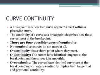
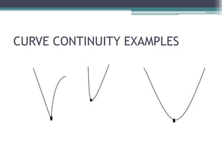
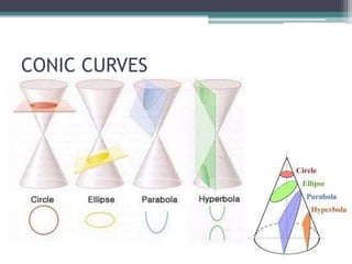
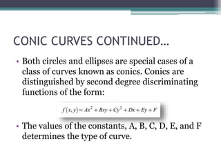
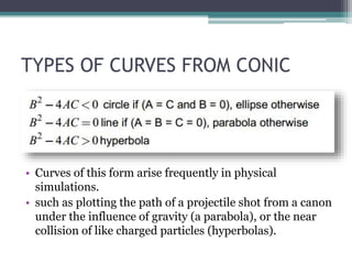
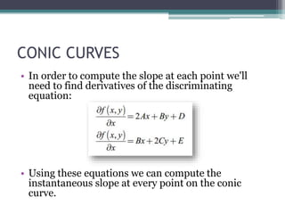
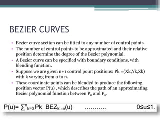
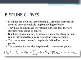
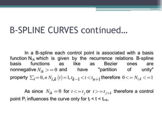
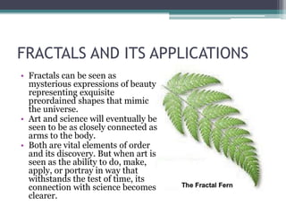
This document provides an introduction to different types of curves used in computer graphics. It discusses curve continuity, conic curves such as parabolas and hyperbolas, piecewise curves, parametric curves, spline curves, Bezier curves, B-spline curves, and applications of fractals. Key points covered include the four types of continuity, how conic curves are defined by discriminant functions, using control points to define piecewise, spline, Bezier and B-spline curves, and properties of Bezier curves such as passing through the first and last control points.

1. INTRODUCTION TO THE CURVES
COMPUTER GRAPHICS
UNIT V
-BY MS. ARTI GAVAS

2. CURVE CONTINUITY
• A breakpoint is where two curve segments meet within a
piecewise curve.
• The continuity of a curve at a breakpoint describes how those
curves meet at the breakpoint.
• There are four possible types of continuity
• No continuity: curves do not meet at all.
• C0continuity : its a sharp point where they meet.
• C1 continuity: The curves have identical tangents at the
breakpoint and the curves join smoothly.
• Cn continuity: The curves have identical curvature at the
breakpoint and curvature continuity implies both tangential
and positional continuity.

3. CURVE CONTINUITY EXAMPLES

4. CONIC CURVES

5. CONIC CURVES CONTINUED…
• Both circles and ellipses are special cases of a
class of curves known as conics. Conics are
distinguished by second degree discriminating
functions of the form:
• The values of the constants, A, B, C, D, E, and F
determines the type of curve.

6. TYPES OF CURVES FROM CONIC
• Curves of this form arise frequently in physical
simulations.
• such as plotting the path of a projectile shot from a canon
under the influence of gravity (a parabola), or the near
collision of like charged particles (hyperbolas).

7. CONIC CURVES
• In order to compute the slope at each point we'll
need to find derivatives of the discriminating
equation:
• Using these equations we can compute the
instantaneous slope at every point on the conic
curve.

8. PIECEWISE CURVE DESIGN
• The order of the curve determines the minimum number of control
points necessary to define the curve.
• We must have at least order control points to define a curve. To
make curves with more than order control points, you can join two
or more curve segments into a piecewise curve

9. PARAMETRIC CURVE DESIGN
• A parametric curve that lies in a plane is defined by two
functions, x(t) and y(t), which use the independent
parameter t.
• x(t) and y(t) are coordinate functions, since their values
represent the coordinates of points on the curve.
• As t varies, the coordinates (x(t), y(t)) sweep out the
curve.
• As an example consider the two functions:
• x(t) = sin(t)
• y(t) = cos(t)
• As t varies from zero to 360, a circle is swept out by (x(t),
y(t)).

10. PARAMETRIC CURVE DESIGN example

11. SPLINE CURVE REPRESENTATION
• A spline curve is a mathematical representation for
which it is easy to build an interface that will allow a user
to design and control the shape of complex curves and
surfaces.
• The general approach is that the user enters a sequence
of points, and a curve is constructed whose shape closely
follows this sequence.
• The points are called control points. A curve that
actually passes through each control point is called an
interpolating curve.
• A curve that passes near to the control points but not
necessarily through them is called an approximating
curve.

12. SPLINE CURVE REPRESENTATION

13. BEZIER CURVES
• Bezier curve section can be fitted to any number of control points.
• The number of control points to be approximated and their relative
position determine the degree of the Bezier polynomial.
• A Bezier curve can be specified with boundary conditions, with
blending function.
• Suppose we are given n+1 control point positions: Pk =(Xk,Yk,Zk)
with k varying from 0 to n.
• These coordinate points can be blended to produce the following
position vector P(u) , which describes the path of an approximating
Bezier polynomial function between P0 and Pn.

14. BEZIER CURVES continued…

15. ADVANTAGEOUS OF BAZIER CURVES
• Easy to implement
• Reasonably powerful in curve design.
• Efficient methods for determining coordinate positions
along a Bezier curve can be set up using recursive
calculations.

16. PROPERTIES OF BAZIER CURVES
• Bezier curves are always passes through the first and last
control points.
• The slope at the beginning of the curve is along the line
joining the first two control points and the slope at the
end of the curve is along the line joining the last two end
points.
• It lies within the convex hull of the control points.

17. B-SPLINE CURVES
• B-splines are not used very often in 2D graphics software but
are used quite extensively in 3D modeling software.
• They have an advantage over Bezier curves in that they are
smoother and easier to control.
• B-splines consist entirely of smooth curves, but sharp corners
can be introduced by joining two spline curve segments.
• The continuous curve of a b-spline is defined by control
points.
• The equation for k-order B-spline with n+1 control points:

18. B-SPLINE CURVES continued…

19. FRACTALS AND ITS APPLICATIONS
• Fractals can be seen as
mysterious expressions of beauty
representing exquisite
preordained shapes that mimic
the universe.
• Art and science will eventually be
seen to be as closely connected as
arms to the body.
• Both are vital elements of order
and its discovery. But when art is
seen as the ability to do, make,
apply, or portray in way that
withstands the test of time, its
connection with science becomes
clearer.

20. APPLICATIONS
• Nature
• Animations & movies
• Bacteria Cultures
• Biological systems