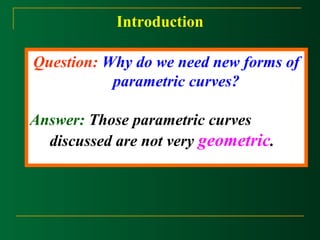
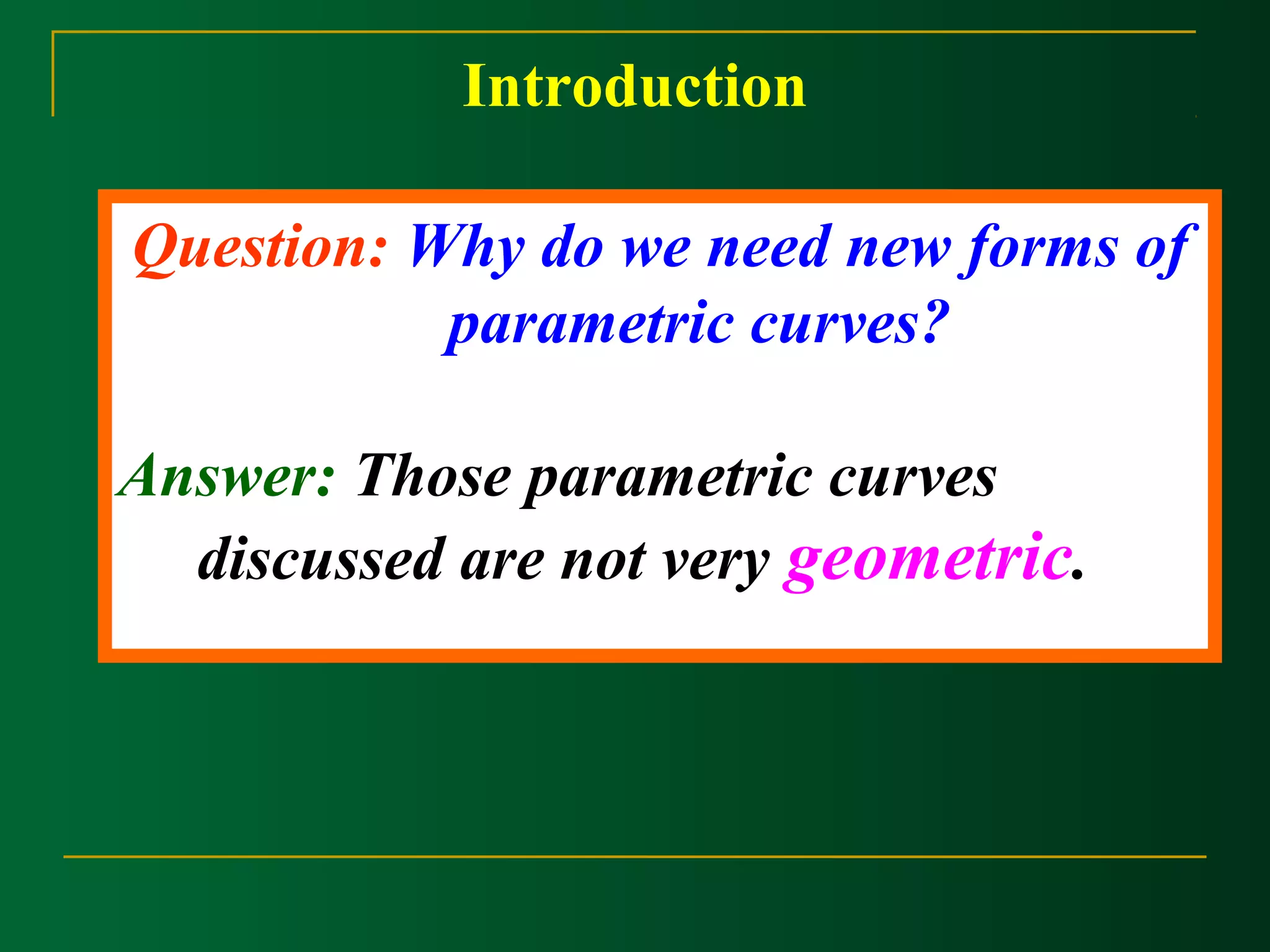
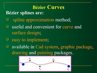
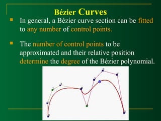
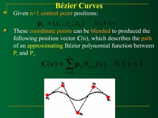
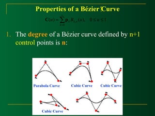
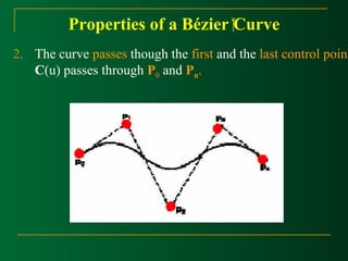
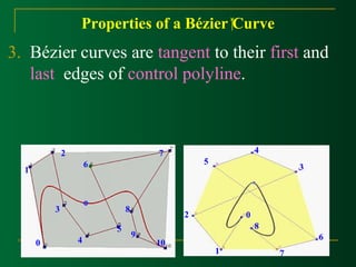
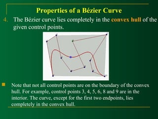
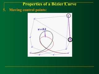
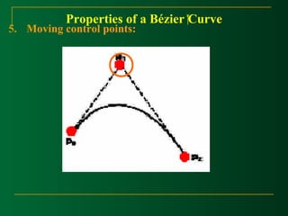
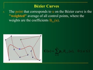
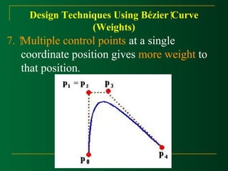
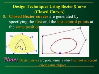
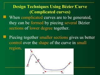
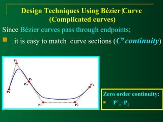
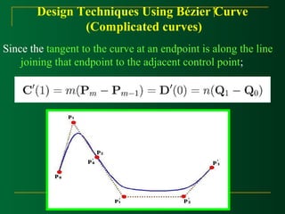
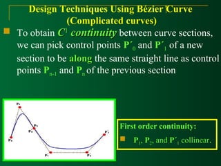
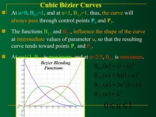
This document discusses Bézier curves and their properties. It begins by stating that traditional parametric curves are not very geometric and do not provide intuitive shape control. It then outlines desirable properties for curve design systems, including being intuitive, flexible, easy to use, providing a unified approach for different curve types, and producing invariant curves under transformations. The document proceeds to discuss Bézier, B-spline and NURBS curves which address these properties by allowing users to manipulate control points to modify curve shapes. Key properties of Bézier curves are described, including their basis functions and the fact that moving control points modifies the curve smoothly. Cubic Bézier curves are discussed in detail as a common parametric curve type, and


![Cubic Bézier Curves
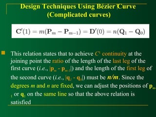
At the end positions of the cubic Bézier curve, The
parametric first and second derivatives are:
(0) 3( 2 ), (1) 3( ) 1 0 3 2 C¢ = p - p C¢ = p - p
(0) 6( 2 ), (1) 6( 2 ) 0 1 2 1 2 3 C¢¢ = p - p + p C¢¢ = p - p + p
With C1 and C2 continuity between sections, and by
expanding the polynomial expressions for the blending
functions: the cubic Bézier point function in the matrix form:
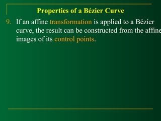
[ ]
ù
ú ú ú ú
û
é
ê ê ê ê
ë
= × ×
0
1
2
3
( ) 3 2 1
p
p
p
p
C MBez u u u u
1 3 3 1
ù
ú ú ú ú
û
é
ê ê ê ê
ë
- -
-
-
=
3 6 3 0
3 3 0 0
1 0 0 0
Bez M](https://image.slidesharecdn.com/curvemodeling-beziercurves-141127024556-conversion-gate01/85/Curve-modeling-bezier-curves-38-320.jpg)


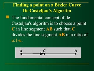
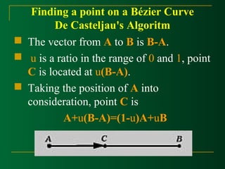
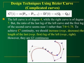
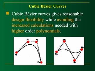
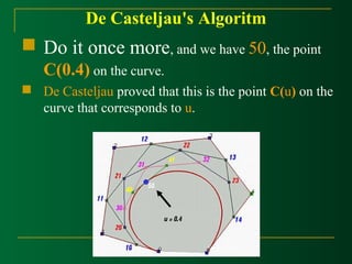
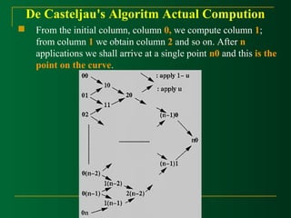
![De Casteljau's Algoritm
Casteljau's algorithm: we want to find C(u), where u
is in [0,1].
Starting with the first polyline, 00-01-02-03…-0n, use the
formula to find a point 1i on the leg from 0i to 0(i+1) that
divides the line segment in a ratio of u:1-u. we ill obtain n
point 10,11,12,…,1(n-1), they defind a new polyline of n-1
legs.](https://image.slidesharecdn.com/curvemodeling-beziercurves-141127024556-conversion-gate01/85/Curve-modeling-bezier-curves-43-320.jpg)
![De Casteljau's Algoritm
Casteljau's algorithm: we want to find C(u), where u
is in [0,1].
Starting with the first polyline, 00-01-02-03…-0n, use the
formula to find a point 1i on the leg from 0i to 0(i+1) that
divides the line segment in a ratio of u:1-u. we ill obtain n
point 10,11,12,…,1(n-1), they defind a new polyline of n-1
legs.](https://image.slidesharecdn.com/curvemodeling-beziercurves-141127024556-conversion-gate01/85/Curve-modeling-bezier-curves-44-320.jpg)


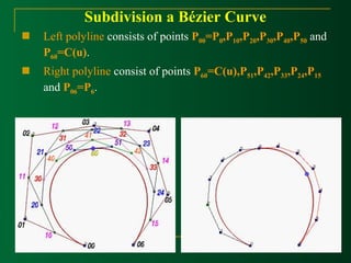
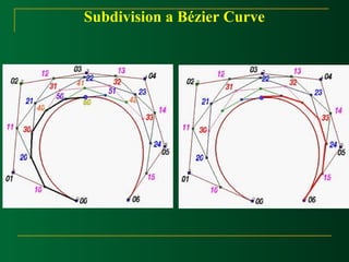
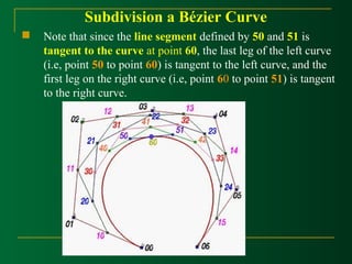
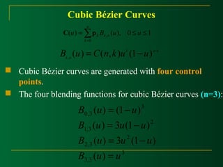
![Subdivision a Bézier Curve
Given s set of n+1 control points P0,p1,P2, …,Pn and a
parameter value u in the range of 0 and 1, we wannt to find
two sets of n+1 control points Q0,Q1,Q2, ..,Qn and R0,R1,R2,
…,Rn such that the Bézier curve definde by Qi’s (resp. Ri’s) is
the piece of the original Bézier curve on [0,u] (resp., [u,1]).](https://image.slidesharecdn.com/curvemodeling-beziercurves-141127024556-conversion-gate01/85/Curve-modeling-bezier-curves-51-320.jpg)