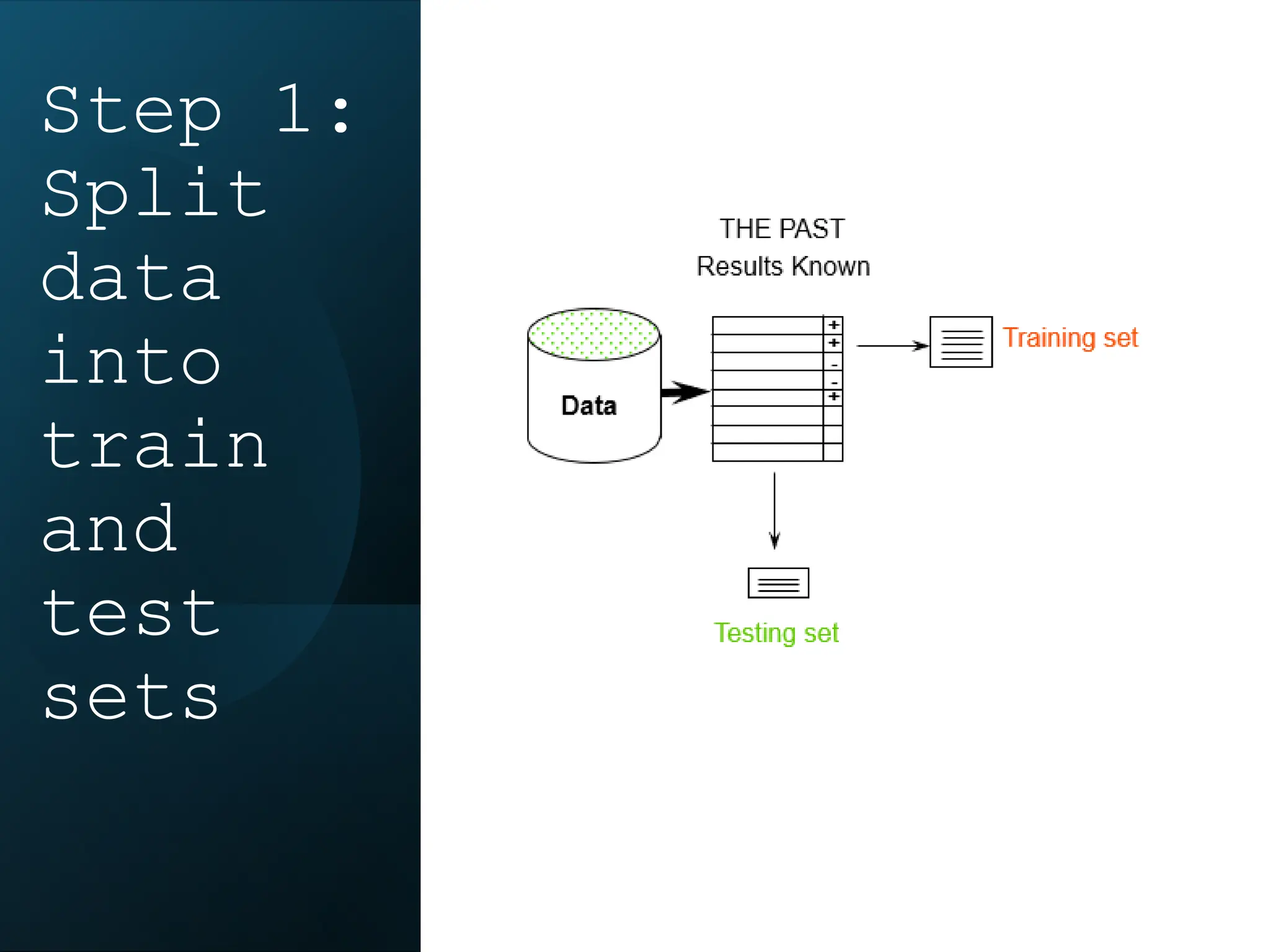
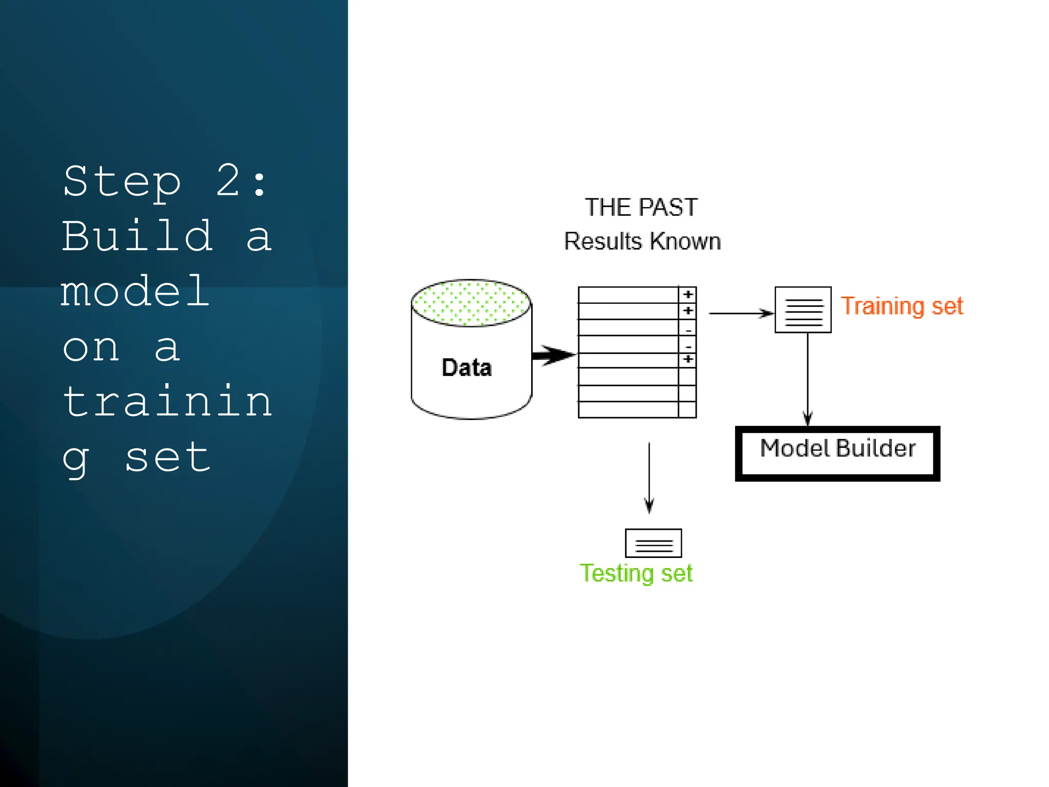
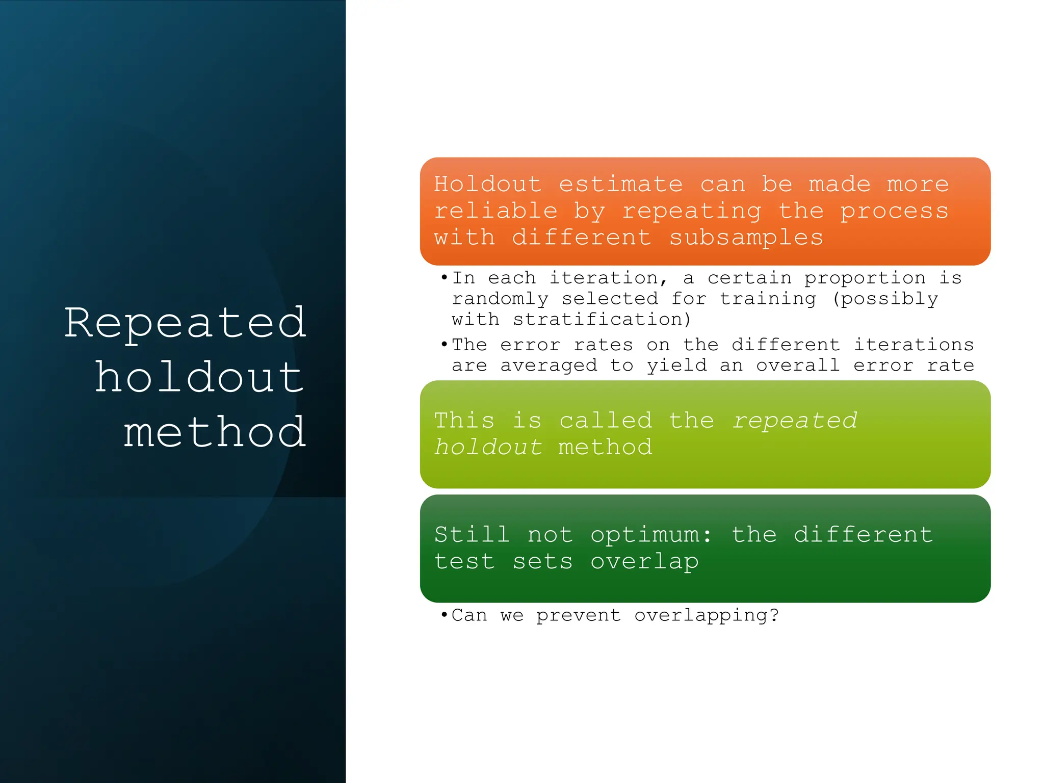
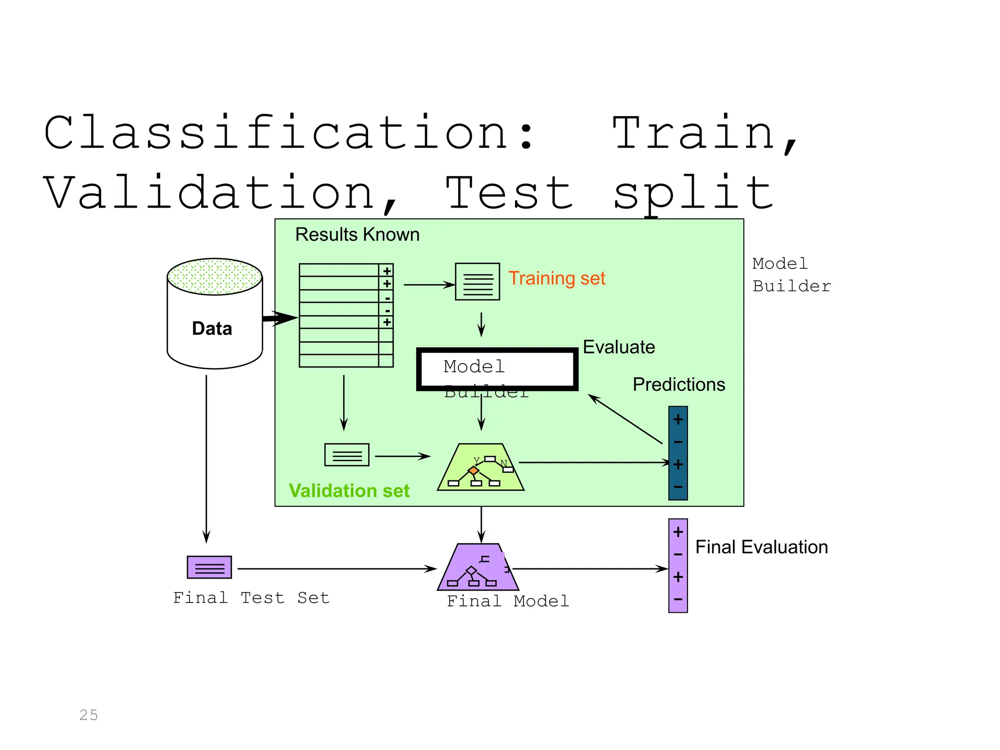
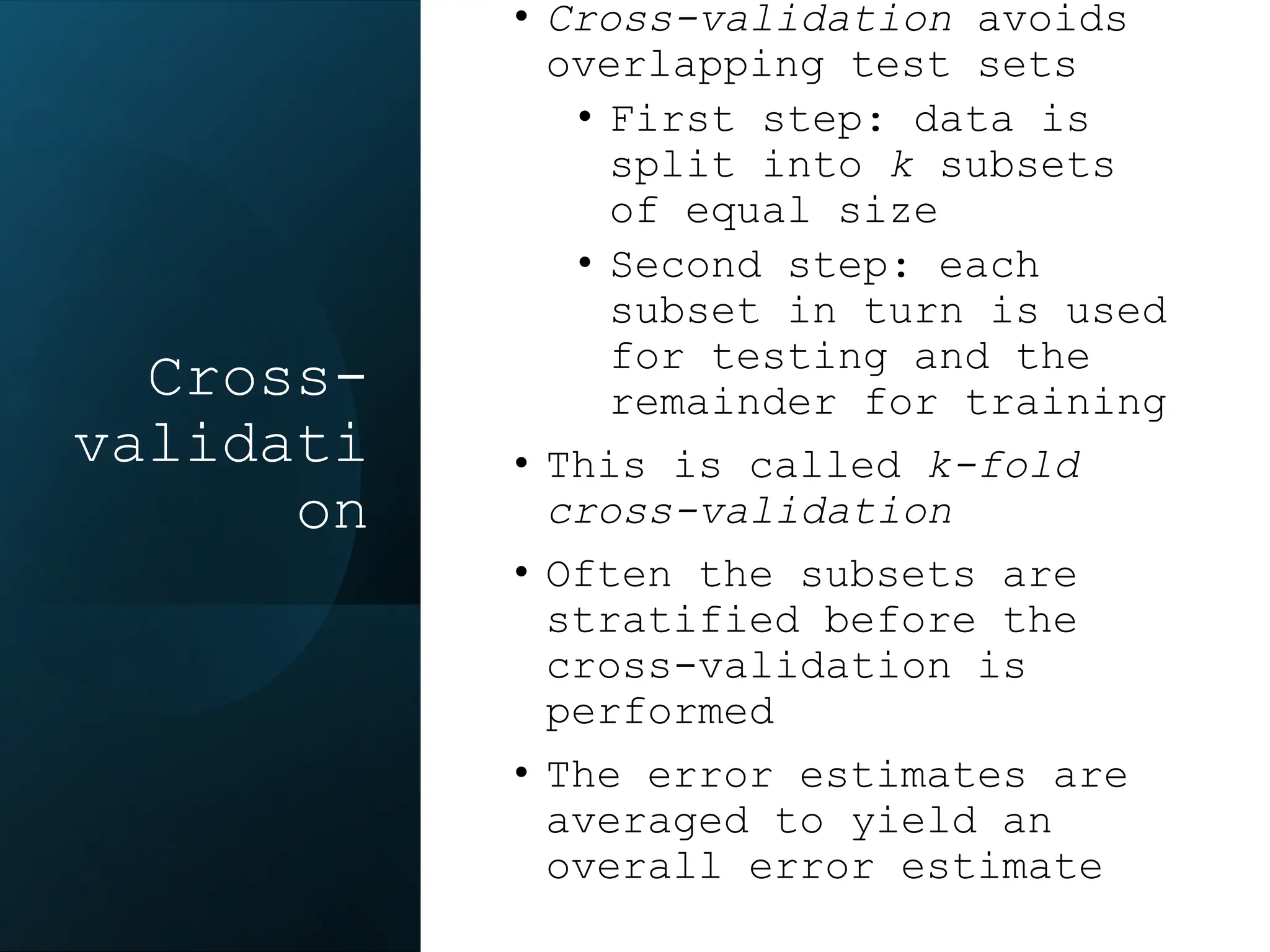
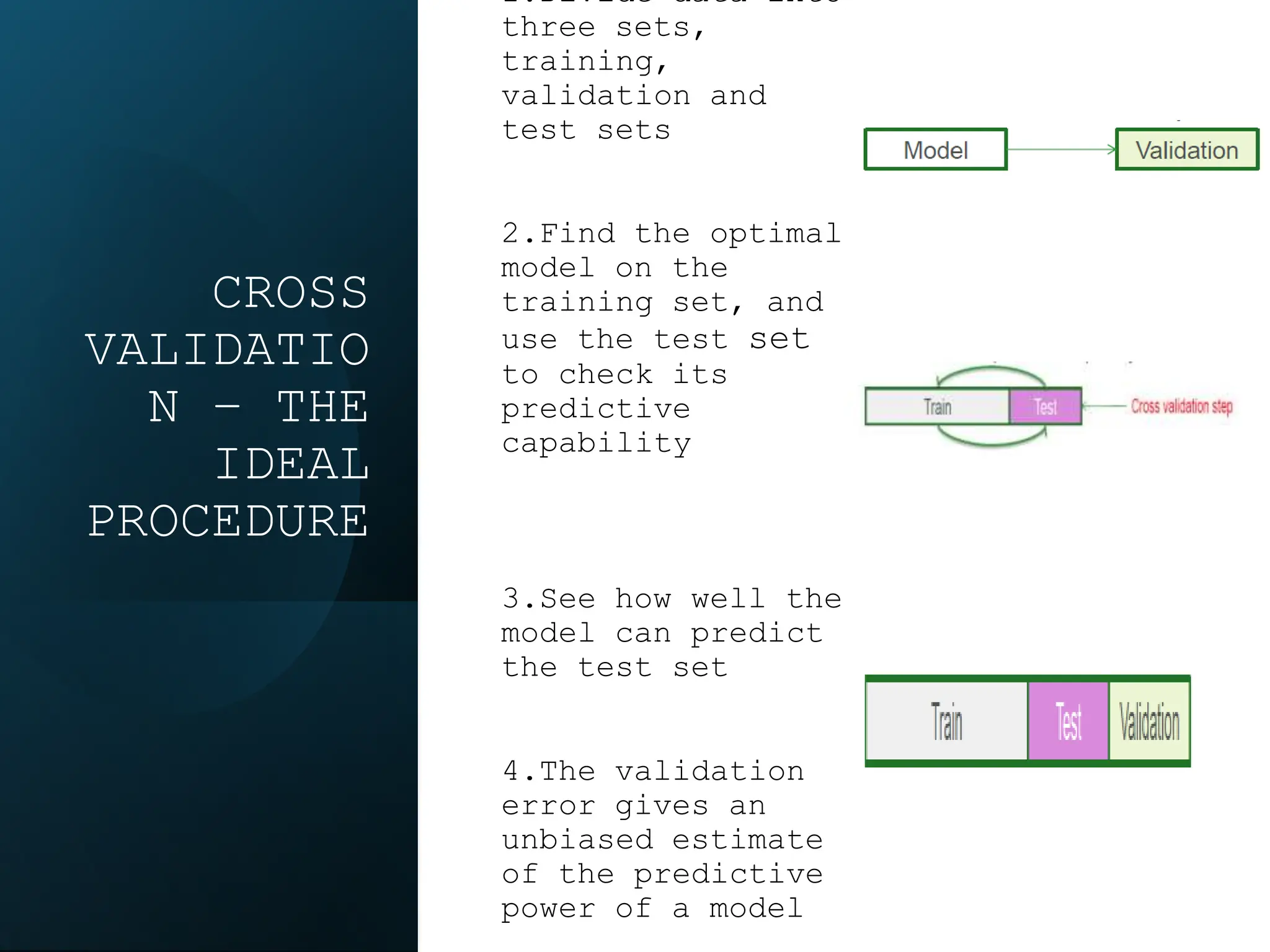
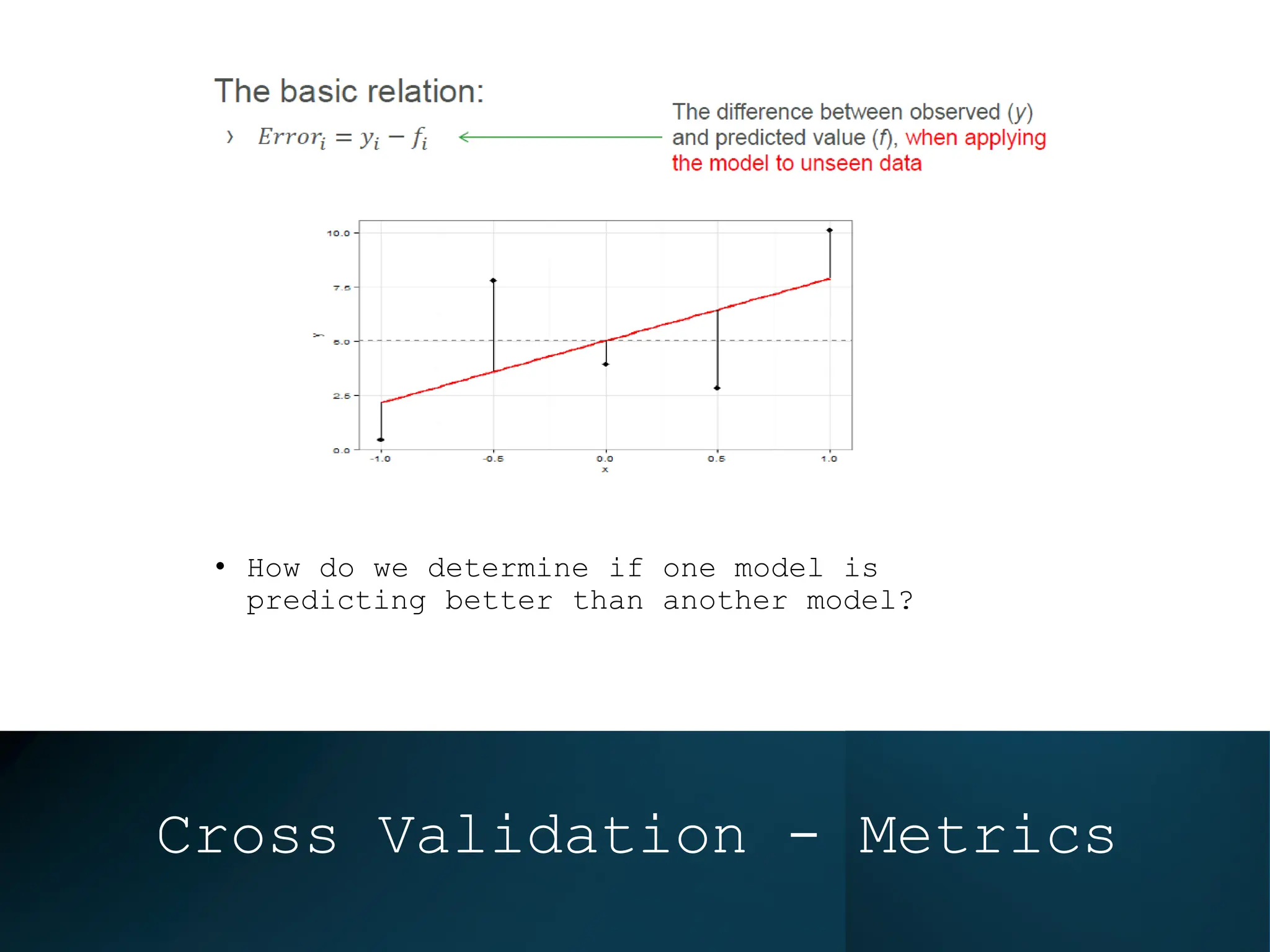
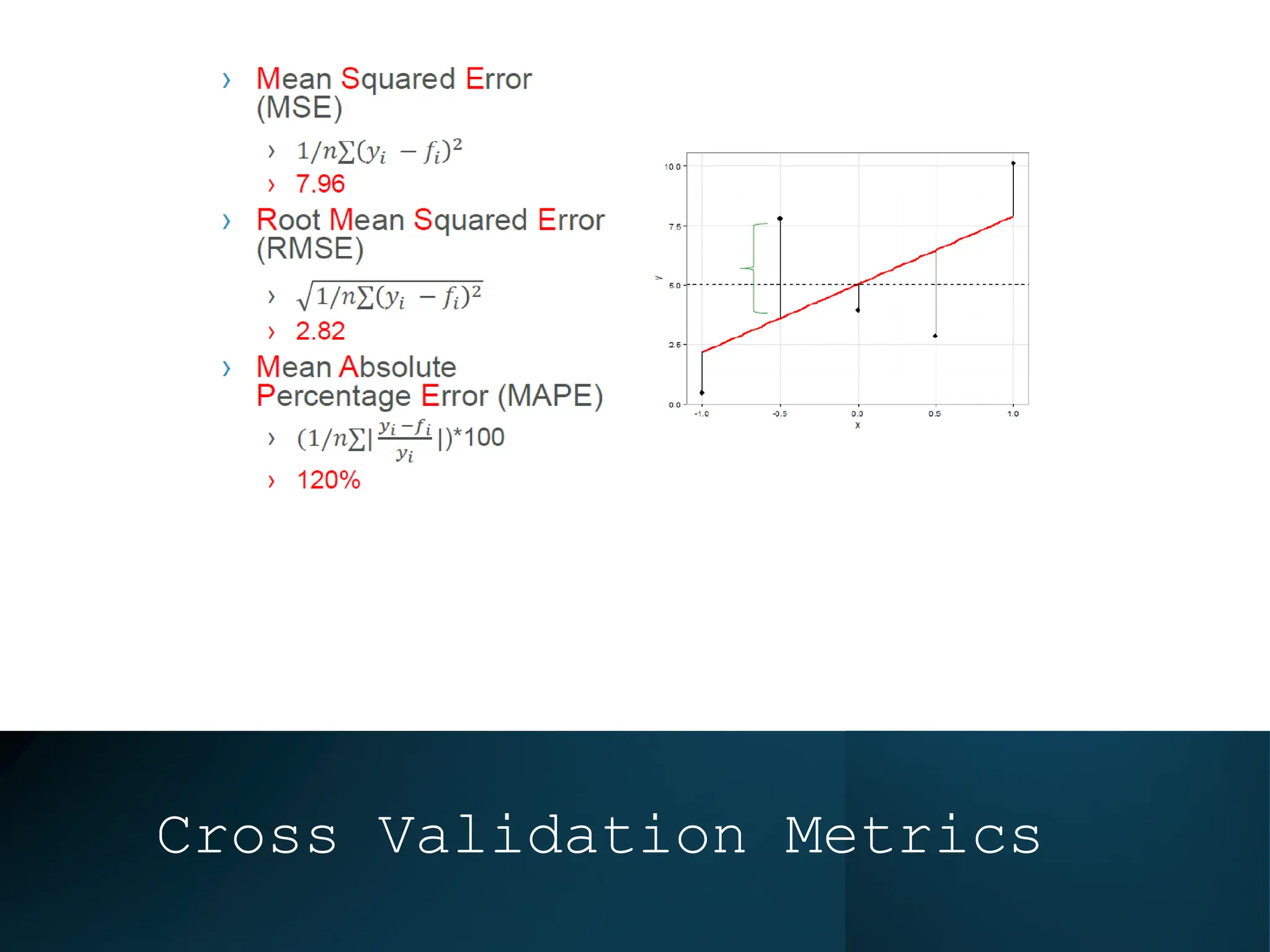
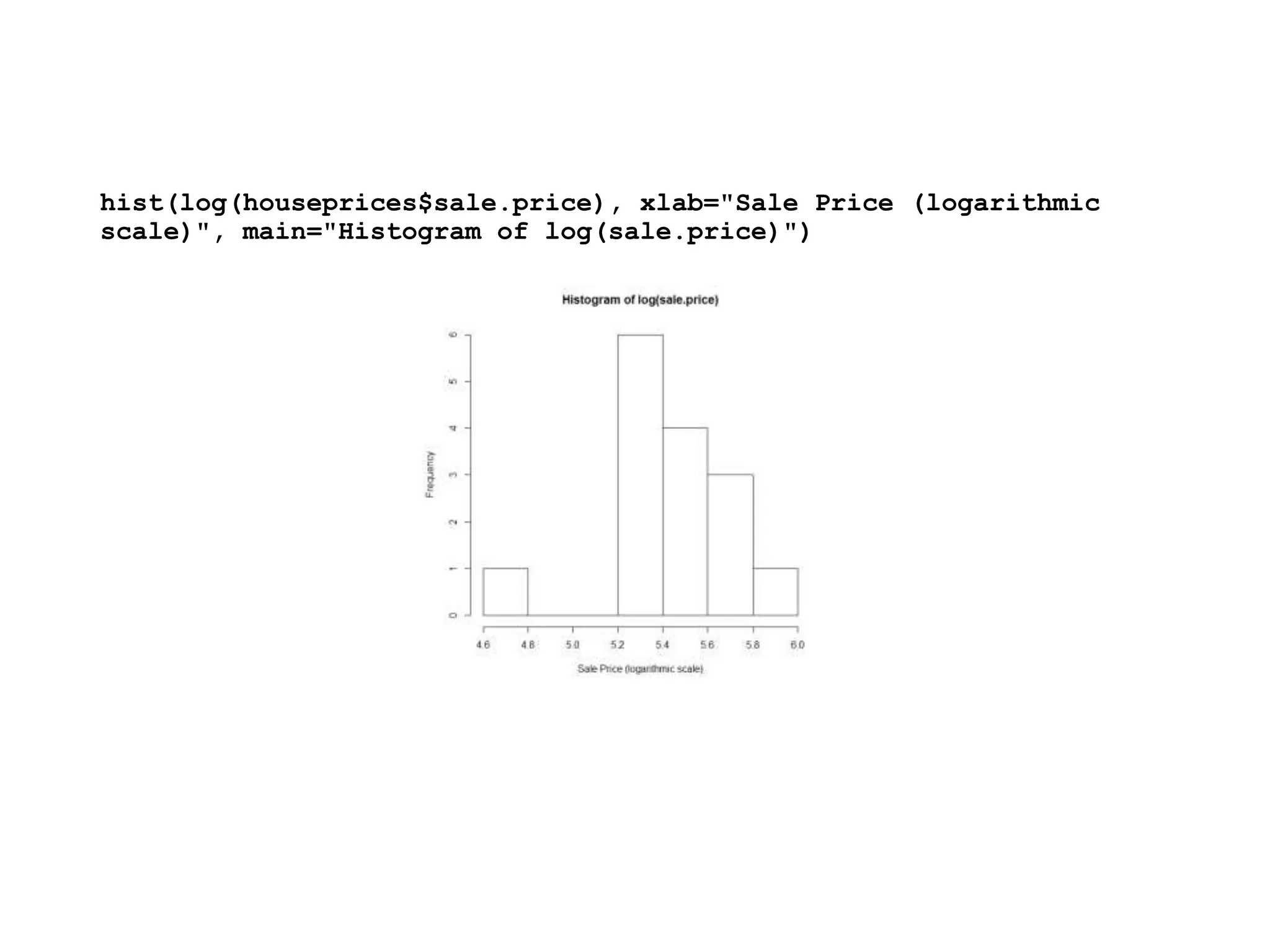
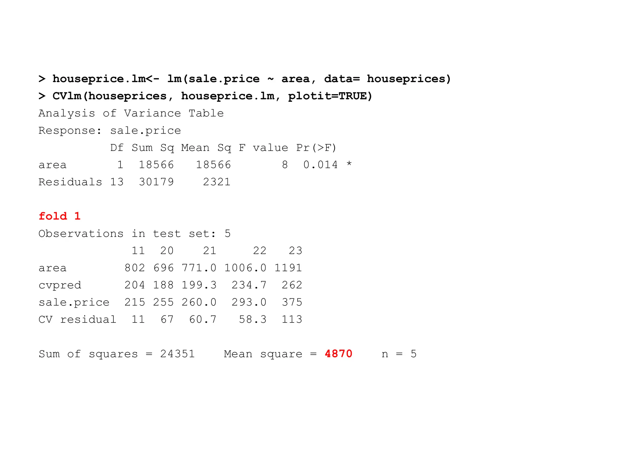
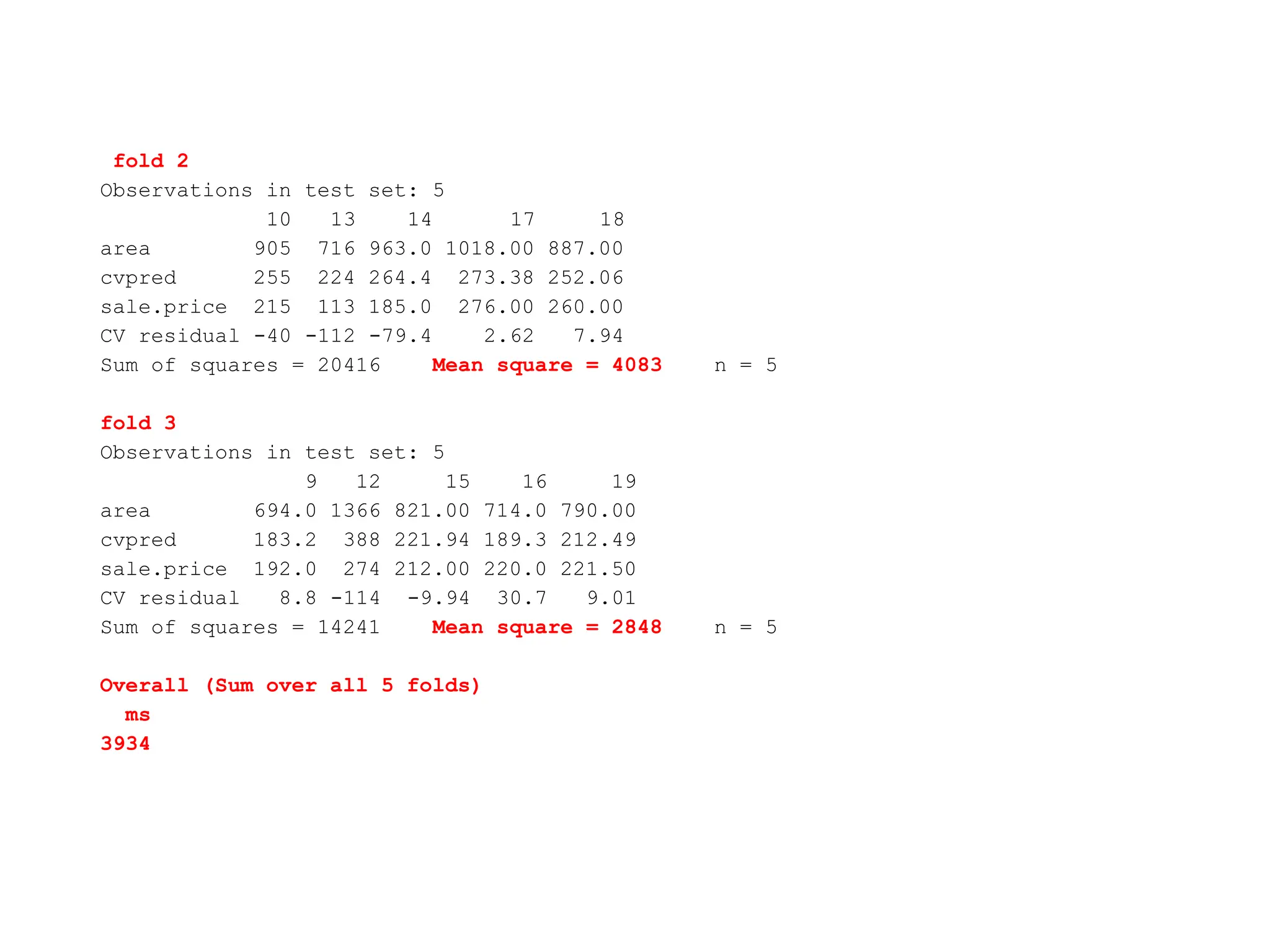
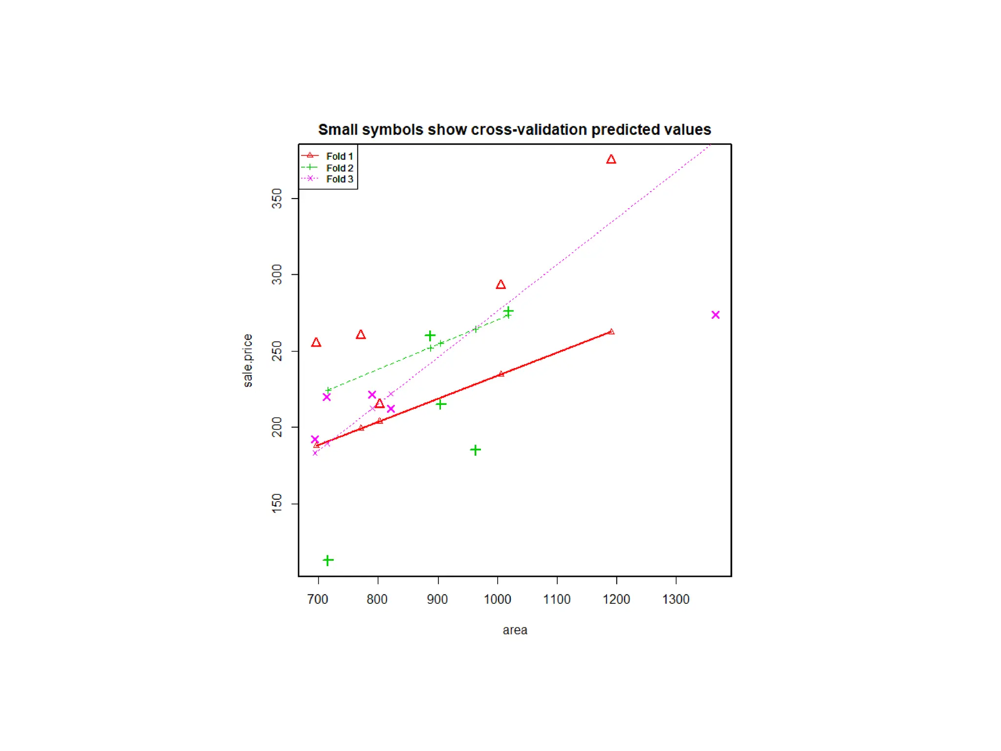
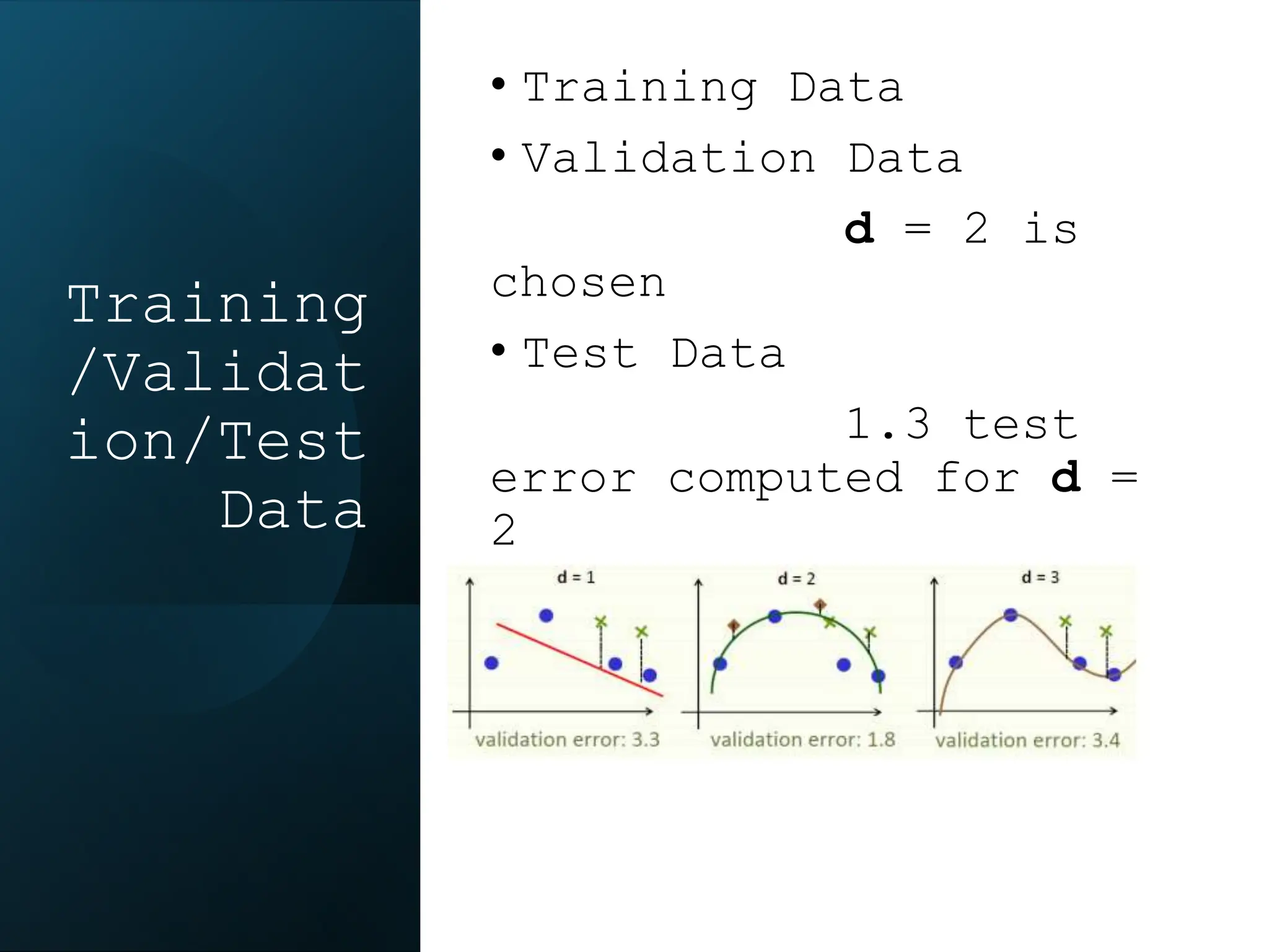
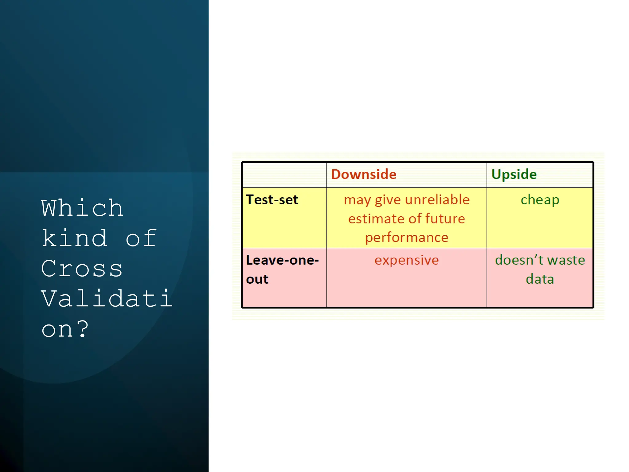
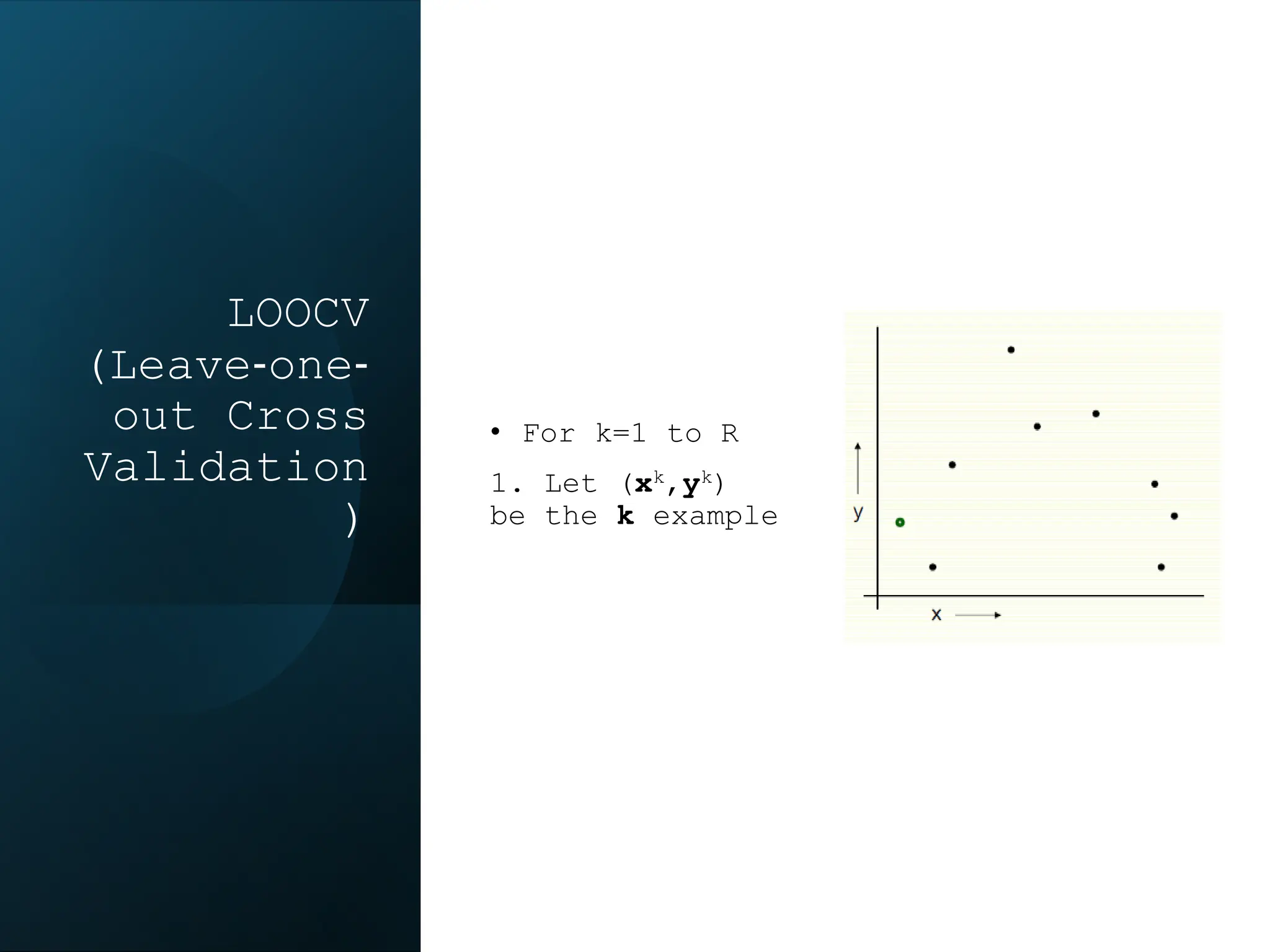
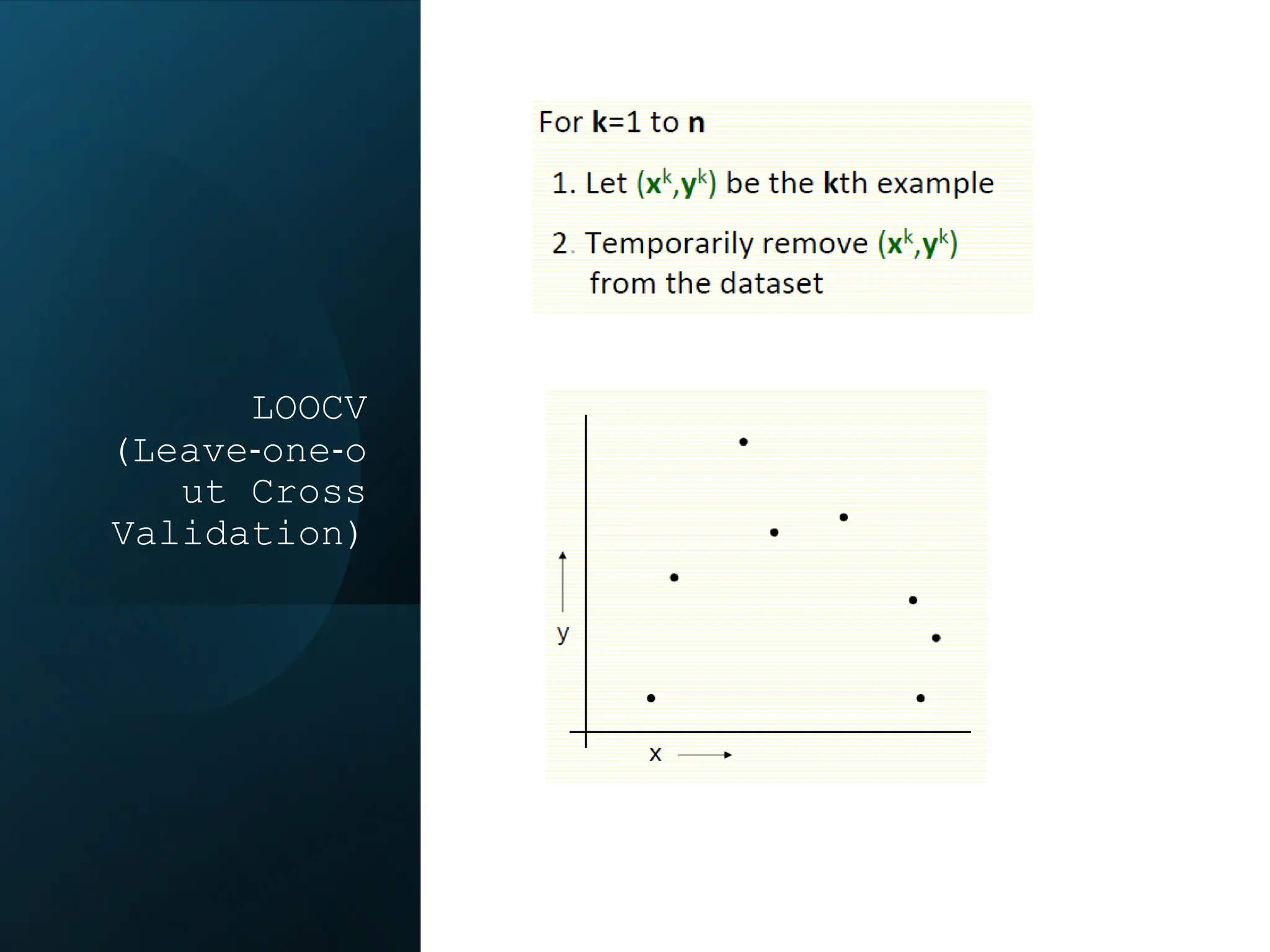
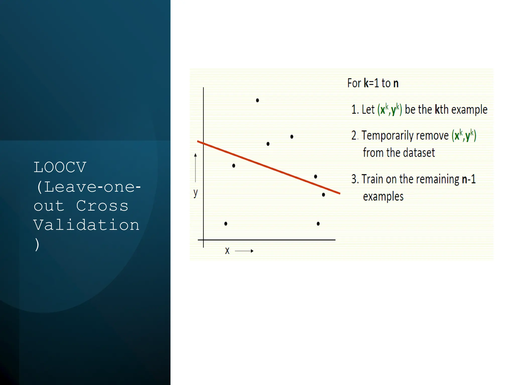
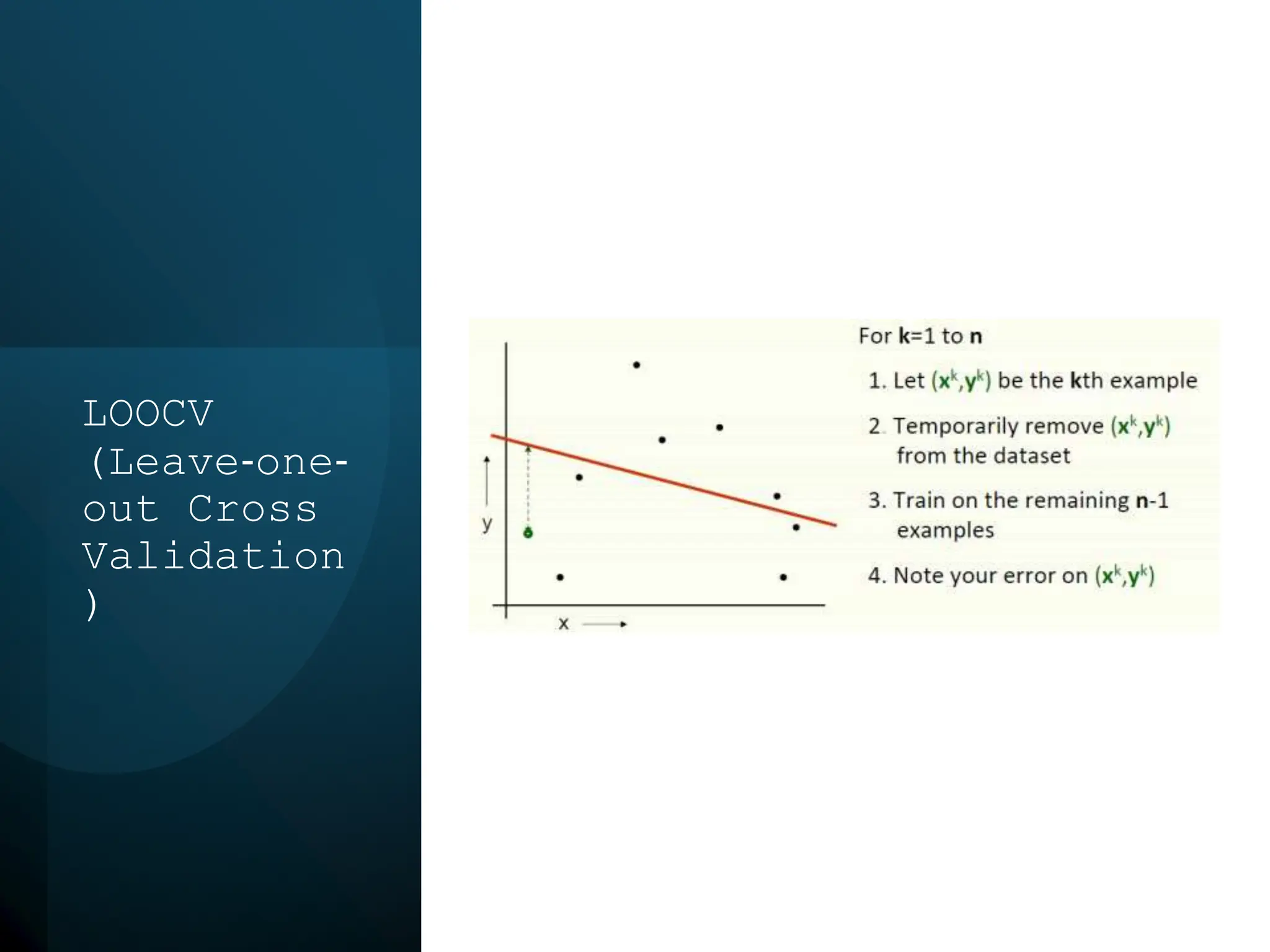
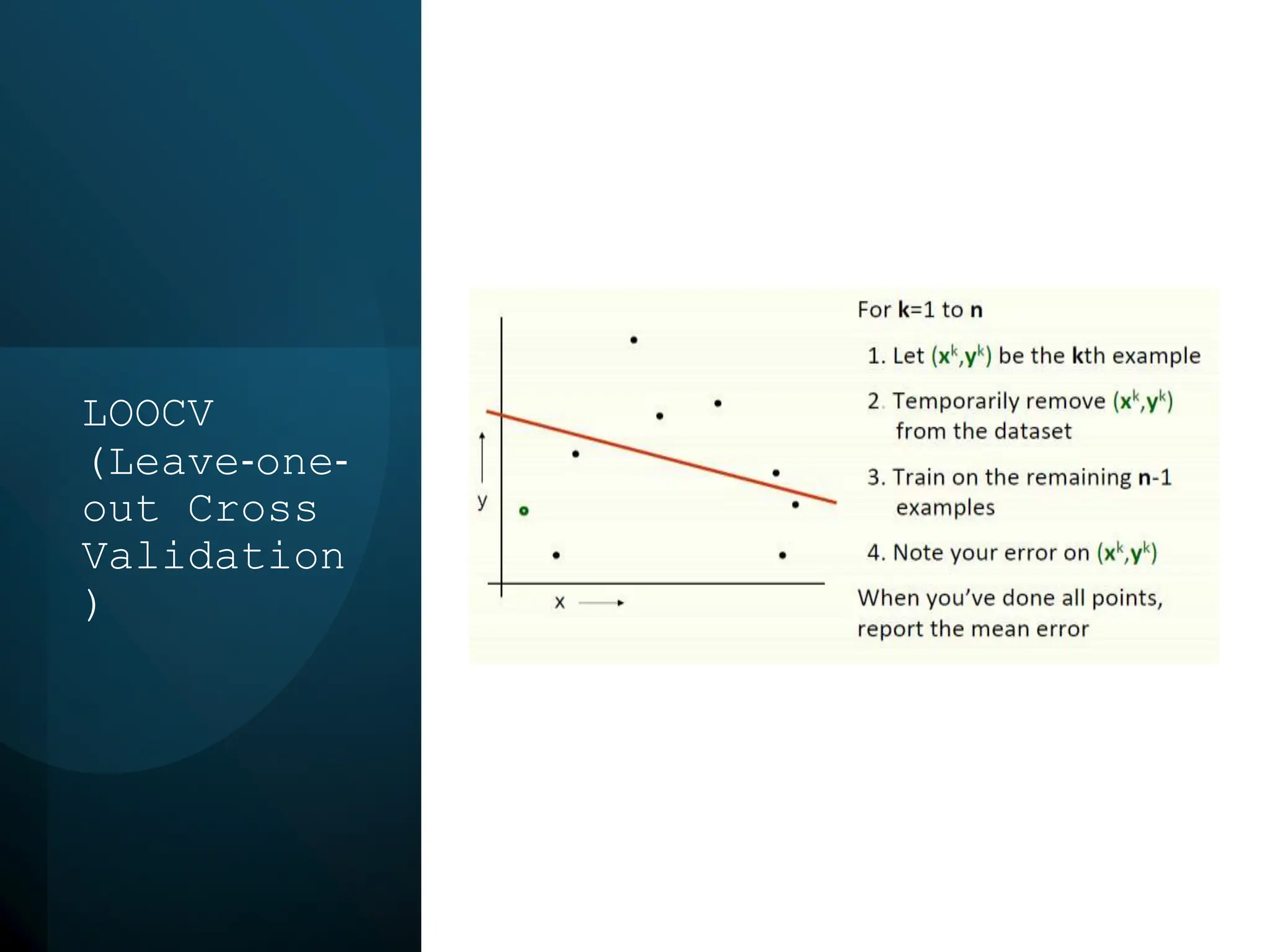
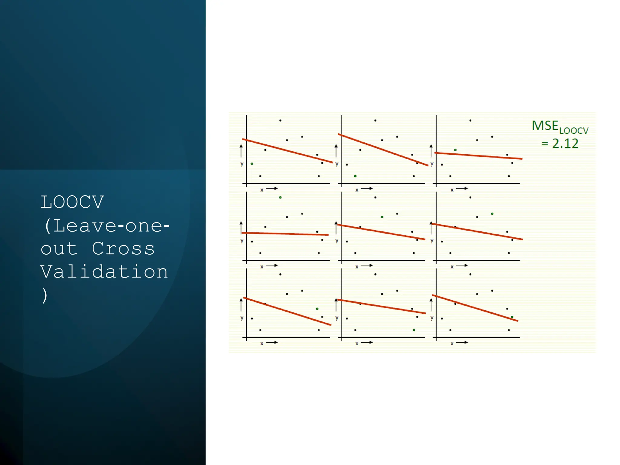
This document discusses statistical learning and model selection. It introduces statistical learning problems, statistical models, the need for statistical modeling, and issues around evaluating models. Key points include: statistical learning involves using data to build a predictive model; a good model balances bias and variance to minimize prediction error; cross-validation is described as the ideal procedure for evaluating models without overfitting to the test data.

1. Statistical
Learning and
Model
Selection
By
Dr. Sampada K S
Associate Professor
Dept. of CSE, RNSIT

2. learning
theory not
only a tool
for
theoretical
analysis but
also a tool
for creating
practical
algorithms
for
estimating
multidimensi
onal
functions.
• Examples of the learning problems are:
• Predict whether a patient, hospitalized due
to a heart attack, will have a second heart
attack.
• The prediction is to be based on demographic, diet and
clinical measurements for that patient.
• Predict the price of a stock in 6 months from
now,
• on the basis of company performance measures and
economic data.
• Estimate the amount of glucose in the blood
of a diabetic person,
• from the infrared absorption spectrum of that person’s
blood.
• Identify the risk factors for prostate cancer,
• based on clinical and demographic variables.

3. A statistical
learning
problem is
learning from
the data.
• we have an outcome measurement, usually
• quantitative
• categorical
• We have a Training Set which is used to
observe the outcome and feature
measurements for a set of objects.
• Using this data we build a Prediction Model,
or a Statistical Learner, which enables us to
predict the outcome for a set of new unseen
objects.

4. What is
statisti
cal
model?
• Modeling is an art, as well as a science
and, is directed toward finding a good
approximating model … as the basis for
statistical inference
• A statistical model is a type of
mathematical model that comprises of
the assumptions undertaken to describe
the data generation process.
• Type of mathematical model? Statistical model is
non-deterministic unlike other mathematical
models where variables have specific values.
Variables in statistical models are stochastic i.e.
they have probability distributions.
• Assumptions? But how do those assumptions
us understand the properties or characteristics of
the true data? Simply put, these assumptions
make it easy to calculate the probability of an
event.

5. Why Do
We Need
Statisti
cal
Modeling
?
• The statistical model plays a fundamental role in
carrying out statistical inference which helps in
making propositions about the unknown properties
and characteristics of the population as below:
• Estimation
• The estimator is a random variable in itself,
whereas an estimate is a single number which
gives us an idea of the distribution of the data
generation process.
• Confidence Interval
• It gives an error bar around the single estimate
number i.e. a range of values to signify the
confidence in the estimate arrived on the basis
of a number of samples. For example, estimate
A is calculated from 100 samples and has a
wider confidence interval, whereas estimate B
is calculated from 10000 samples and thus has
a narrower confidence interval

6. A good learner is one
that accurately
predicts such an
outcome.

7. The
formulat
ion of
the
learning
problem
• Two main types of problems are that of
• Regression Estimation: The problem
problem of regression estimation is the
problem of minimizing the risk functional
with the squared error loss function.
• Classification: When the problem is of
problem is of classification, the loss
function is an indicator function. Hence
the problem is that of finding a function
that minimizes the misclassification error

8. PREDICTION ACCURACY
A good learner is the one which has good
prediction accuracy; in other words, which has
the smallest prediction error.

9. • The data at hand is to be used to find the best predictive model.
• Almost all predictive modeling techniques have tuning parameters
that enable the model to flex to find the structure in the data.
• Hence, we must use the existing data to identify settings for the
model’s parameters that yield the best and most realistic
predictive performance (known as model tuning) for the future.
• Traditionally, this has been achieved by splitting the existing data
into training and test sets.
• The training set is used to build and tune the model and the test
set is used to estimate the model’s predictive performance.
• Modern approaches to model building split the data into multiple
training and test sets, which have often been shown to get more
optimal tuning parameters and give a more accurate
representation of the model’s predictive performance.

10. The Problem of Over-
fitting
• Data includes both
patterns (stable,
underlying
relationships) and
noise (transient,
random effects).
• Noise has no predictive
value; so a model is
over-fit when it
incorporates noise.
• The figure below right
shows results from two
predictive models—
polynomial and linear—
applied to the same
data set.
• The polynomial model
predicts sales almost
50 times the actual
value, where the linear
model is far more

11. Bias and Variance of
the Estimator
The best learner is the one which can balance
the bias and the variance of a model.

12. • In most situations, however, the
true distributions are unknown
and must be estimated from
data.
• Parameter Estimation (we saw the
Maximum Likelihood Method)
• Assume a particular form for the
density (e.g. Gaussian), so only the
parameters (e.g., mean and variance)
need to be estimated
• Maximum Likelihood
• Bayesian Estimation
• Non-parametric Density
Estimation (not covered)
• Assume NO knowledge about the
density
• Kernel Density Estimation
• Nearest Neighbor Rule
• .

13. prediction
(averaged
over all
data sets)
differs from
the desired
regression
function.
Variance
measures how
much the
predictions
for
individual
data sets
vary around
their
average.

14. Bias and
variance move
in opposing
directions and
at a suitable
bias-variance
combination
the PE is the
minimum in the
test data. The
model that
achieves this
lowest
possible PE is
the best
prediction model.

15. Evaluation and
Credibility
How much should we believe in what was
learned?

16. • Possible
evaluation
measures:
• Classification
Accuracy
• Total cost/benefit
– when different
errors involve
different costs
• Error in numeric
predictions
• How reliable are
the predicted
results ?
Evaluat
ion
issues

17. examples are
available,
including several
hundred examples
from each class,
then a simple
evaluation is
sufficient
• Randomly split data
into training and
test sets (usually
2/3 for train, 1/3
for test)
• Build a classifier
using the train
set and evaluate
Evaluat
ion

18. Step 1:
Split
data
into
train
and
test
sets

19. Step 2:
Build a
model
on a
trainin
g set

20. Step 3:
Evaluat
e on
test
set
(Re-
train?)

21. Evaluati
on on
“small”
data
• The holdout method reserves a
certain amount for testing and
uses the remainder for training
• Usually: one third for testing,
the rest for training
• For small or “unbalanced”
datasets, samples might not be
representative
• Few or none instances of some
classes
• Stratified sample: advanced
version of balancing the data
• Make sure that each class is
represented with approximately
equal proportions in both
subsets
21

22. Handling
unbalanc
ed data
• The training set is used to train the learner. The test set
is used to estimate the error rate of the trained model.
• This method has two basic drawbacks.
• the error estimate is not stable.
• in case of 'bad' split, the estimate is not reliable.
22

23. Repeated
holdout
method
Holdout estimate can be made more
reliable by repeating the process
with different subsamples
•In each iteration, a certain proportion is
randomly selected for training (possibly
with stratification)
•The error rates on the different iterations
are averaged to yield an overall error rate
This is called the repeated
holdout method
Still not optimum: the different
test sets overlap
•Can we prevent overlapping?

24. A note
on
paramete
r tuning
It is important
that the test data
is not used in any
way to create the
classifier
Some learning
schemes operate in
two stages:
Stage 1: builds the
basic structure
Stage 2: optimizes
parameter settings
The test data can’t
be used for
parameter tuning!
Proper procedure
uses three sets:
training data,
validation data,
and test data
Validation data is
used to optimize
parameters

25. 25
Classification: Train,
Validation, Test split
Data
Predictions
Y N
Results Known
Training set
Validation set
+
+
-
-
+
Model
Builder
Evaluate
+
-
+
-
Final Model
Final Test Set
+
-
+
-
Final Evaluation
Model
Builder

26. Cross-
validati
on
• Cross-validation avoids
overlapping test sets
• First step: data is
split into k subsets
of equal size
• Second step: each
subset in turn is used
for testing and the
remainder for training
• This is called k-fold
cross-validation
• Often the subsets are
stratified before the
cross-validation is
performed
• The error estimates are
averaged to yield an
overall error estimate

27. CROSS
VALIDATIO
N – THE
IDEAL
PROCEDURE
1.Divide data into
three sets,
training,
validation and
test sets
2.Find the optimal
model on the
training set, and
use the test set
to check its
predictive
capability
3.See how well the
model can predict
the test set
4.The validation
error gives an
unbiased estimate
of the predictive
power of a model

28. TRAINING/TE
ST DATA
SPLIT
data in training/test
sets
• training data is
used to fit parameters
• test data is used to
assess how classifier
generalizes to new
data
What if classifier has
“non‐tunable”
parameters?
• a parameter is
“non‐tunable” if
tuning (or training)
it on the training
data leads to

29. TRAINING/TE
ST DATA
SPLIT
What about test error? Seems
appropriate
• degree 2 is the best model
according to the test error
Except what do we report as the
test error now?
• Test error should be computed
on data that was not used for
training at all
• Here used “test” data for
training, i.e. choosing model

30. VALIDATIO
N DATA
Same question when
choosing among several
classifiers
• our polynomial degree
example can be looked at
as choosing among 3
classifiers (degree 1, 2,
or 3)
• Solution: split the
labeled data into three
parts

31. TRAINING/ VALIDATION

32. K-FOLD
CROSS
VALIDATIO
N
›Since data are often scarce,
there might not be enough to set
aside for a validation sample
›To work around this issue k-fold
CV works as follows:
1. Split the sample into k
subsets of equal size
2. For each fold estimate a
model on all the subsets except
one
3. Use the left out subset to
test the model, by calculating a
CV metric of choice
4. Average the CV metric
across subsets to get the CV error
›This has the advantage of using
all data for estimating the model,
however finding a good value for k
can be tricky

33. K-fold Cross Validation
Example
1.Split the data
into 5 samples
2.Fit a model to
the training
samples and use
the test sample
to calculate a
CV metric.
3.Repeat the
process for the
next sample,
until all
samples have
been used to
either train or
test the model

34. Which kind of Cross
Validation?

35. Improve
cross-
validati
on
• Even better: repeated cross-
validation
Example:
10-fold cross-validation is
repeated 10 times and results are
averaged (reduce the variance)

36. Cross Validation - Metrics
• How do we determine if one model is
predicting better than another model?

37. Cross Validation Metrics

38. Best
Practi
ce for
Report
ing
Model
Fit
1.Use Cross Validation to
find the best model
2.Report the RMSE and MAPE
statistics from the cross
validation procedure
3.Report the R Squared from
the model as you normally
would.
The added cross-validation
information will allow one
to evaluate not how much
variance can be explained
by the model, but also the
predictive accuracy of the
model. Good models should
have a high predictive AND
explanatory power!

39. EXAMPLE
• The following table gives the size of the floor area (ha)
and the price ($000), for 15 houses sold in the Canberra
(Australia) suburb of Aranda in 1999.
• For simplicity, we will use 3-fold cross validation
> library(DAAG)
Loading required package: lattice
> data(houseprices)
> summary(houseprices)
area bedrooms sale.price
Min. : 694.0 Min. :4.000 Min. :112.7
1st Qu.: 743.5 1st Qu.:4.000 1st Qu.:213.5
Median : 821.0 Median :4.000 Median :221.5
Mean : 889.3 Mean :4.333 Mean :237.7
3rd Qu.: 984.5 3rd Qu.:4.500 3rd Qu.:267.0
Max. :1366.0 Max. :6.000 Max. :375.0

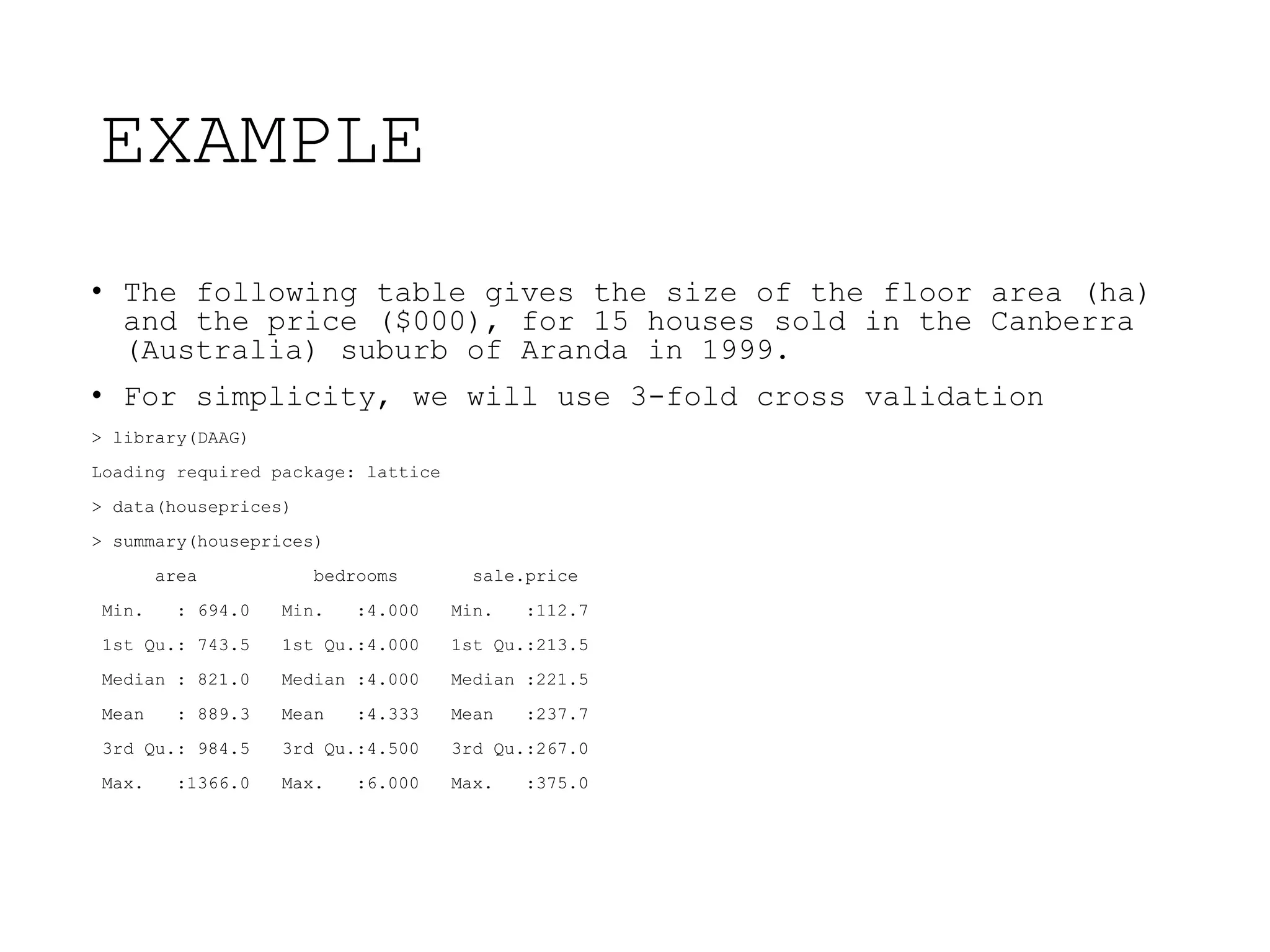
40. > houseprices$bedrooms=as.factor(houseprices[,2])
> summary(houseprices)
area bedrooms sale.price
Min. : 694.0 4:11 Min. :112.7
1st Qu.: 743.5 5: 3 1st Qu.:213.5
Median : 821.0 6: 1 Median :221.5
Mean : 889.3 Mean :237.7
3rd Qu.: 984.5 3rd Qu.:267.0
Max. :1366.0 Max. :375.0
plot(sale.price ~ area, data = houseprices, log = "y",pch = 16, xlab = "Floor
Area", ylab = "Sale Price", main = "log(sale.price) vs area")

41. hist(log(houseprices$sale.price), xlab="Sale Price (logarithmic
scale)", main="Histogram of log(sale.price)")

42. > #Split row numbers randomly into 3 groups
> rand<- sample(1:15)%%3 + 1
> # a%%3 is a remainder of a modulo 3
> #Subtract from a the largest multiple of 3 that is <= a; take
remainder
> (1:15)[rand == 1] # Observation numbers from the first group
[1] 2 3 5 7 12
> (1:15)[rand == 2] # Observation numbers from the second group
[1] 4 8 9 11 14
> (1:15)[rand == 3] # Observation numbers from the third group
[1] 1 6 10 13 15

43. > houseprice.lm<- lm(sale.price ~ area, data= houseprices)
> CVlm(houseprices, houseprice.lm, plotit=TRUE)
Analysis of Variance Table
Response: sale.price
Df Sum Sq Mean Sq F value Pr(>F)
area 1 18566 18566 8 0.014 *
Residuals 13 30179 2321
fold 1
Observations in test set: 5
11 20 21 22 23
area 802 696 771.0 1006.0 1191
cvpred 204 188 199.3 234.7 262
sale.price 215 255 260.0 293.0 375
CV residual 11 67 60.7 58.3 113
Sum of squares = 24351 Mean square = 4870 n = 5

44. fold 2
Observations in test set: 5
10 13 14 17 18
area 905 716 963.0 1018.00 887.00
cvpred 255 224 264.4 273.38 252.06
sale.price 215 113 185.0 276.00 260.00
CV residual -40 -112 -79.4 2.62 7.94
Sum of squares = 20416 Mean square = 4083 n = 5
fold 3
Observations in test set: 5
9 12 15 16 19
area 694.0 1366 821.00 714.0 790.00
cvpred 183.2 388 221.94 189.3 212.49
sale.price 192.0 274 212.00 220.0 221.50
CV residual 8.8 -114 -9.94 30.7 9.01
Sum of squares = 14241 Mean square = 2848 n = 5
Overall (Sum over all 5 folds)
ms
3934

46. Training
/Validat
ion/Test
Data
• Training Data
• Validation Data
d = 2 is
chosen
• Test Data
1.3 test
error computed for d =
2

47. Which
kind of
Cross
Validati
on?

48. MEASURING
THE MODEL
ACCURACY
48

49. MEASURING
THE MODEL
ACCURACY
49

50. 50
More on cross-
validation
• Standard method for evaluation:
stratified ten-fold cross-
validation
• Why ten? Extensive experiments have
shown that this is the best choice
to get an accurate estimate
• Stratification reduces the
estimate’s variance
• Even better: repeated stratified
cross-validation
• E.g. ten-fold cross-validation is
repeated ten times and results are
witten & eibe

51. 51
Leave-One-Out cross-
validation
• Leave-One-Out:
a particular form of cross-validation:
• Set number of folds to number of training instances
• I.e., for n training instances, build classifier n times
• Makes best use of the data
• Involves no random subsampling
• Very computationally expensive
• (exception: NN)

52. LOOCV
(Leave‐one‐
out Cross
Validation
)
• For k=1 to R
1. Let (xk,yk)
be the k example

53. LOOCV
(Leave‐one‐o
ut Cross
Validation)

54. LOOCV
(Leave‐one‐
out Cross
Validation
)

55. LOOCV
(Leave‐one‐
out Cross
Validation
)

56. LOOCV
(Leave‐one‐
out Cross
Validation
)

57. LOOCV
(Leave‐one‐
out Cross
Validation
)