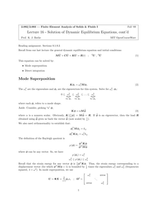
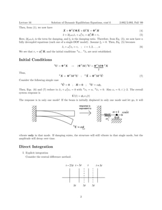
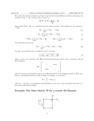
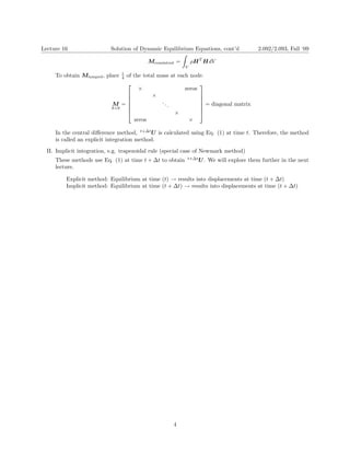
The lecture covers the solution of dynamic equilibrium equations in finite element analysis, focusing on mode superposition, direct integration methods, and their applications. It details the use of eigenvalues and eigenvectors, the development of decoupled equations for each mode, and the methods for explicit and implicit integration. Key concepts include the role of damping, the impact of initial conditions, and the significance of stability in numerical methods.

1. 2.092/2.093 — Finite Element Analysis of Solids & Fluids I Fall ‘09
Lecture 16 -Solution of Dynamic Equilibrium Equations, cont’d
Prof. K. J. Bathe MIT OpenCourseWare
Reading assignment: Sections 9.1-9.3
Recall from our last lecture the general dynamic equilibrium equation and initial conditions:
0
MU ¨+ CU˙ + KU = R(t); 0U , U˙ (1)
This equation can be solved by:
Mode superposition
•
Direct integration
•
Mode Superposition
Kφi = ωi 2Mφi (2)
The ωi 2 are the eigenvalues and φi are the eigenvectors for this system. Solve for ωi 2 , φi:
ω2 ω2 ≤ ... ≤ ω2
12n
0 ≤ |{z} ≤ |{z} |{z}
for φ1 for φ2 for φn
where each φi refers to a mode shape.
Aside: Consider, picking “a” φ, Kφ = αMφ˜(3)
1
where α is a nonzero scalar. Obviously, K α φ = Mφ˜= R. If φ˜is an eigenvector, then the load R
1
obtained using φ˜gives us back the vector φ˜(now scaled by α ). We also used orthonormality to establish that:
φTi Mφj = δij
φTi Kφj = ωi 2δij
The definition of the Rayleigh quotient is
φT Kφ
ρ (φ)=
φT Mφ
where φ can be any vector. So, we have ρ (φi)= ωi 2
ω12 ≤ ρ (φi) ≤ ωn 2 Recall that the strain energy for any vector φ is 12 φT Kφ. Thus, the strain energy corresponding to a displacement vector (for which φT Mφ = 1) is bounded by 21 times the eigenvalues ω12 and ωn 2 (frequencies squared, λ = ω2). In mode superposition, we use
⎡⎤
ω2 zeros
1
U = ΦX =Σ n φixi ; Ω2 = ⎢⎣ ... ⎥⎦
i=1
zeros ω2
n 1

2. Lecture 16 Solution of Dynamic Equilibrium Equations, cont’d 2.092/2.093, Fall ‘09
Then, from (1), we now have X ¨+ ΦT CΦX˙ + Ω2X = ΦT R (4)
x¨+2ξiωix˙i + ωi 2 xi = φiT R = ri (5) Here, 2ξiωix˙i is the term for damping, and ξi is the damping ratio. Therefore, from Eq. (5), we now have n fully decoupled equations (each one of a single-DOF model). Assume ξi = 0. Then, Eq. (5) becomes
x¨i + ωi 2 xi = ri ; i =1, 2,...,n (6) We see that ri = φTi R, and the initial conditions 0xi , 0x˙i are next established.
Initial Conditions
0U = Φ 0X (ΦT M ) 0U = ΦT MΦ 0X
→
|
{z
}
I
Thus,
0X
=
ΦT M
0U
;
0 ˙X = ΦT
M 0 ˙U
(7)
Consider the following simple case
0 ˙U
= 0
;
R = 0
;
0U
=
αφ1
Then, Eqs. (6) and (7) reduce to x¨1 + ω12x1 = 0 with 0x1 = α, 0x˙1 = 0. Also xi = 0, i ≥ 2. The overall system response is U (t)= φ1x1(t) The response is in only one mode! If the beam is initially displaced in only one mode and let go, it will
vibrate only in that mode. If damping exists, the structure will still vibrate in that single mode, but the amplitude will decay over time.
Direct Integration
I. Explicit integration
Consider the central difference method:
2

3. Lecture 16 Solution of Dynamic Equilibrium Equations, cont’d 2.092/2.093, Fall ‘09
We assume the solution is known up to time t and use the central difference method to determine the solution at time t +Δt. At time t, Eq. (1) gives us
M tU ¨+ C tU˙ + K| {z tU} = tR
tFI
The internal forces, tFI , are calculated from the element stresses. The unknown in the equation is t+ΔtU:
U˙ = 1
t+ΔtU − t−ΔtUt
(A) 2Δt
1
Δt Δt
tU ¨
U˙ − U˙
t+ t−
(a)
2 2
=
Δt
1 1
Δt Δt
U˙
=
U˙
=
t+ΔtU − tU − t−ΔtUt+ tU , t−
(b)
2 2
Δt Δt
Now substitute (b) into (a):
tU ¨= 1
t+ΔtU − 2 tU + t−ΔtU
(B) (Δt)2
Use Eqs. (A) and (B) in Eq. (1) applied at time t to obtain (c1M + c2C) t+ΔtU = tRˆ
(8) where c1 and c2 are constants, and tRˆ is constructed from known values. Next, assume C = 0, and
M is diagonal.
⎤
⎡ ⎢⎢⎢⎢⎢⎣
×
× zeros .
..
zeros
×
×
⎥⎥⎥⎥⎥⎦
M =
Then (8) involves no factorization and is very efficiently solved. If one diagonal element in M is zero, however, the method would not work! Actually, for stability, we must have
TnΔt ≤ =Δtcritical
π
where Tn = ω2π n and ωn is the highest natural frequency. If we use a time step greater than Δtcritical the solution will diverge quickly.
Example: The Mass Matrix M for a 4-node 2D Element 3

4. Z
Lecture 16 Solution of Dynamic Equilibrium Equations, cont’d 2.092/2.093, Fall ‘09
Mconsistent = ρHT HdV
V
To obtain Mlumped, place 14 of the total mass at each node.
⎤
⎡
× zeros ×
M =
8×8
⎢⎢⎢⎢⎢⎣ ⎥⎥⎥⎥⎥⎦
= diagonal matrix . ..
×
zeros
×
In the central difference method, t+ΔtU is calculated using Eq. (1) at time t. Therefore, the method is called an explicit integration method.
II. Implicit integration, e.g. trapezoidal rule (special case of Newmark method)
These methods use Eq. (1) at time t +Δt to obtain t+ΔtU . We will explore them further in the next lecture.
Explicit method: Equilibrium at time (t) results into displacements at time (t +Δt)
→
Implicit method: Equilibrium at time (t +Δt) results into displacements at time (t +Δt)
→ 4

5. MIT OpenCourseWare
http://ocw.mit.edu
2.092 / 2.093 Finite Element Analysis of Solids and Fluids I
Fall 2009
For information about citing these materials or our Terms of Use, visit: http://ocw.mit.edu/terms.