All of material inside is un-licence, kindly use it for educational only but please do not to commercialize it. Based on 'ilman nafi'an, hopefully this file beneficially for you. Thank you.

1. 2.092/2.093 — Finite Element Analysis of Solids & Fluids I Fall ‘09
Lecture 19 -Modeling for Dynamic Analysis & Solution, cont’d
Prof. K. J. Bathe MIT OpenCourseWare
In the last lecture, we discussed two methods for solving this general system:
0
MU ¨+ CU˙ + KU = R(t); 0U , U˙
I. Mode Superposition
p
U =Σ φixi(t)
i=1
So far, we considered the case where p = n.
II. Direct Integration
We concluded that implicit methods are only of interest if they are unconditionally stable.
How many modes do we need to include in the mode superposition method? (What should we select for p?) We consider three cases:
I. Initial Conditions
0U = α1φ1, 0U˙ = 0, R = 0
The response is only in φ1. Therefore, if the initial conditions “use” certain mode shapes only, the response caused by these initial conditions will only be in these certain mode shapes.
II. Loads, Spatial Distribution
0
R = αMφ10U = U˙ = 0
Again, the response is only in φ1 and the conclusion of section I holds here as well.
III. Loads, Frequency Content
x¨i +2ξiωix˙i + ωi 2 xi = sin ˆωt
1

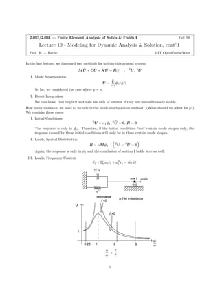
2. Lecture 19 Modeling for Dynamic Analysis Solution, cont’d 2.092/2.093, Fall ‘09
dynamic peak response Dynamic load factor D =
static peak response ˆ
ω, the excitation frequency, is given.
When ˆω is very large, there is no response. When ˆω is very small, the mass follows the excitation, producing a static response.
In actual analysis, Fourier analysis of loads is performed to see what frequencies are contained in the loading.
Step 1: Identify the highest frequency in the loading. The largest ˆω = ωu = ωupper. Define ωco = ωcut-off = 4ωu.
Step 2: Set up a mesh which represents the continuum frequencies accurately up to the cut-off frequency ωco.
How do we know whether enough modes are included? Calculate the error defined by the following:
εp
(t)=
MU¨ p + CU˙ p + KU p − R
2
kRk2
(assume R = 0) 6
where
p
U P =Σ φixi(t)
i=1
A small εp(t) means that we have a good approximation for the solution. Recall: kak2 =Σ
1
(ai)2 2 . If any
i
element of a is large, kak2 will not be small. Therefore, using εp(t) is a good way of assessing whether the dynamic solution obtained is accurate enough.
Static Correction
Consider the load
p
ΔR = R − Σ(Mφiri)
i=1
in a mode superposition solution.
p rˆj = φTj ΔR = φTj R − Σ φTj Mφiri
i=1
p = φjT ΔR = rj − Σ δij ri
i=1
By definition, rˆ= ΦT ΔR. Therefore, for j =1,...,p, we have ˆrj = 0.
2

3. Lecture 19 Modeling for Dynamic Analysis Solution, cont’d 2.092/2.093, Fall ‘09
For a properly modeled problem, the response in ΔR should be at most a static response. Therefore, a good correction ΔUS to the mode superposition solution U P can be obtained from KΔUS =ΔR. Then, the total solution is
U = UP +ΔUS
In practice the mode superposition method is used for problems which have low frequency excitations, such as earthquake response, road excitation analysis, etc. It is ineffective for problems which have very high frequency content such as wave propagation. We will explore this topic next lecture.
3

4. MIT OpenCourseWare
http://ocw.mit.edu
2.092 / 2.093 Finite Element Analysis of Solids and Fluids I
Fall 2009
For information about citing these materials or our Terms of Use, visit: http://ocw.mit.edu/terms.