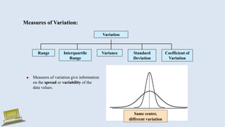
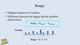
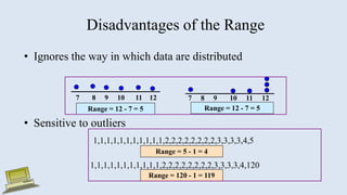
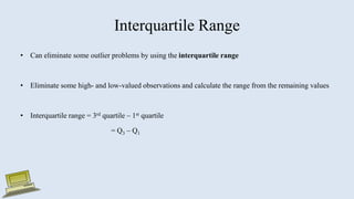
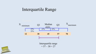
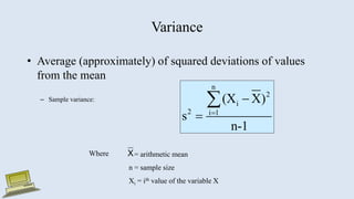
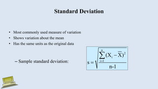
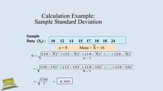
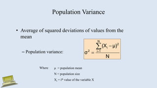
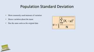
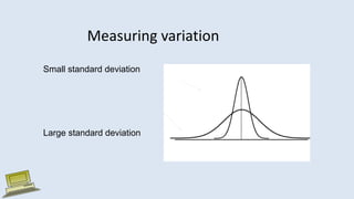
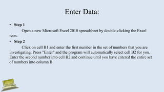
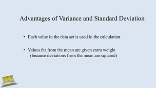
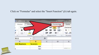
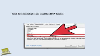
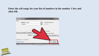
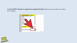
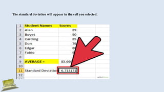
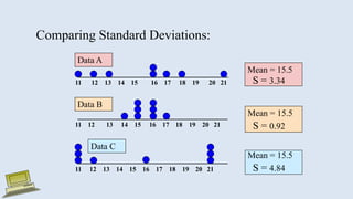
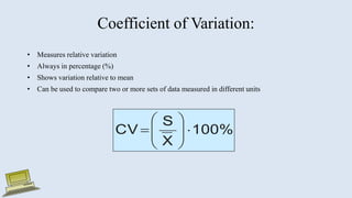
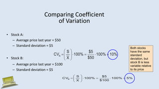
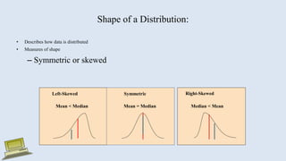
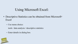
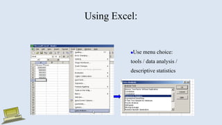
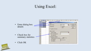
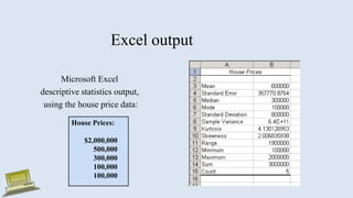
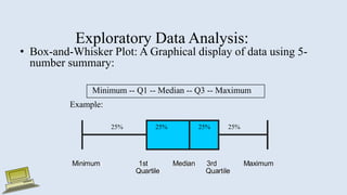
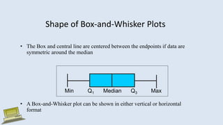
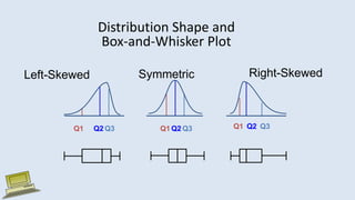
Lecture 3 Dispersion(1).pptx

Lecture 3
Virtual University of Pakistan 1

Contents
Measure of Variation
• Range,
• Standard deviation,
• Variance,
• Inter Quartile Range,
• Coefficient of Variation,
• Box Plot ,
• 5-number summary,
• Real Statistics Add-in ,
• Practical exercise.
Virtual University of Pakistan 2

Objectives
After completing this lecture, you should be able to:
Compute and interpret :
• Range,
• Standard deviation,
• Variance,
• Inter Quartile Range,
• Coefficient of Variation,
• Box Plot.

Same center,
different variation
Measures of Variation:
Variation
Variance Standard
Deviation
Coefficient of
Variation
Range Interquartile
Range
 Measures of variation give information
on the spread or variability of the
data values.

Range:
• Simplest measure of variation
• Difference between the largest and the smallest
observations:
Range = Xlargest – Xsmallest
0 1 2 3 4 5 6 7 8 9 10 11 12 13 14
Range = 14 - 1 = 13
Example:

Disadvantages of the Range
• Ignores the way in which data are distributed
• Sensitive to outliers
7 8 9 10 11 12
Range = 12 - 7 = 5
7 8 9 10 11 12
Range = 12 - 7 = 5
1,1,1,1,1,1,1,1,1,1,1,2,2,2,2,2,2,2,2,3,3,3,3,4,5
1,1,1,1,1,1,1,1,1,1,1,2,2,2,2,2,2,2,2,3,3,3,3,4,120
Range = 5 - 1 = 4
Range = 120 - 1 = 119

Interquartile Range
• Can eliminate some outlier problems by using the interquartile range
• Eliminate some high- and low-valued observations and calculate the range from the remaining values
• Interquartile range = 3rd quartile – 1st quartile
= Q3 – Q1

Interquartile Range
Median
(Q2)
X
maximum
X
minimum Q1 Q3
Example:
25% 25% 25%
25%
12 30 45 57 70
Interquartile range
= 57 – 30 = 27

Variance
• Average (approximately) of squared deviations of values
from the mean
– Sample variance:
n
2
i
2 i 1
(X X)
s
n-1




Where = arithmetic mean
n = sample size
Xi = ith value of the variable X
X

Standard Deviation
• Most commonly used measure of variation
• Shows variation about the mean
• Has the same units as the original data
– Sample standard deviation:
n
2
i
i 1
(X X)
s
n-1





Calculation Example:
Sample Standard Deviation
Sample
Data (Xi) : 10 12 14 15 17 18 18 24
n = 8 Mean = X = 16
2 2 2 2
2 2 2 2
(10 X) (12 X) (14 X) (24 X)
S
n 1
(10 16) (12 16) (14 16) (24 16)
8 1
130
4.309
7
       


       


 

Population Variance
• Average of squared deviations of values from the
mean
– Population variance:
N
μ)
(X
σ
N
1
i
2
i
2




Where μ = population mean
N = population size
Xi = ith value of the variable X

Population Standard Deviation
• Most commonly used measure of variation
• Shows variation about the mean
• Has the same units as the original data
N
μ)
(X
σ
N
1
i
2
i





Measuring variation
Small standard deviation
Large standard deviation

Enter Data:
• Step 1
Open a new Microsoft Excel 2010 spreadsheet by double-clicking the Excel
icon.
• Step 2
Click on cell B1 and enter the first number in the set of numbers that you are
investigating. Press "Enter" and the program will automatically select cell B2 for you.
Enter the second number into cell B2 and continue until you have entered the entire set
of numbers into column B.

Advantages of Variance and Standard Deviation
• Each value in the data set is used in the calculation
• Values far from the mean are given extra weight
(because deviations from the mean are squared)

Click on "Formulas" and select the "Insert Function" (fx) tab again.

Scroll down the dialog box and select the STDEV function

Enter the cell range for your list of numbers in the number 1 box and
click OK

Use the STDEV function to compute the standard deviation. Place your cursor where you wish to
have it appear.

The standard deviation will appear in the cell you selected.

Comparing Standard Deviations:
Mean = 15.5
S = 3.34
11 12 13 14 15 16 17 18 19 20 21
11 12 13 14 15 16 17 18 19 20 21
Data B
Data A
Mean = 15.5
S = 0.92
11 12 13 14 15 16 17 18 19 20 21
Mean = 15.5
S = 4.84
Data C

Coefficient of Variation:
• Measures relative variation
• Always in percentage (%)
• Shows variation relative to mean
• Can be used to compare two or more sets of data measured in different units
100%
X
S
CV 










Comparing Coefficient
of Variation
• Stock A:
– Average price last year = $50
– Standard deviation = $5
• Stock B:
– Average price last year = $100
– Standard deviation = $5
Both stocks
have the same
standard
deviation, but
stock B is less
variable relative
to its price
10%
100%
$50
$5
100%
X
S
CVA 












5%
100%
$100
$5
100%
X
S
CVB 













Shape of a Distribution:
• Describes how data is distributed
• Measures of shape
– Symmetric or skewed
Mean = Median
Mean < Median Median < Mean
Right-Skewed
Left-Skewed Symmetric

Using Microsoft Excel:
• Descriptive Statistics can be obtained from Microsoft®
Excel
– Use menu choice:
tools / data analysis / descriptive statistics
– Enter details in dialog box

Using Excel:
Use menu choice:
tools / data analysis /
descriptive statistics

Using Excel:
• Enter dialog box
details
• Check box for
summary statistics
• Click OK

Excel output
Microsoft Excel
descriptive statistics output,
using the house price data:
House Prices:
$2,000,000
500,000
300,000
100,000
100,000

Exploratory Data Analysis:
• Box-and-Whisker Plot: A Graphical display of data using 5-
number summary:
Minimum -- Q1 -- Median -- Q3 -- Maximum
Example:
Minimum 1st Median 3rd Maximum
Quartile Quartile
Minimum 1st Median 3rd Maximum
Quartile Quartile
25% 25% 25% 25%

Shape of Box-and-Whisker Plots
• The Box and central line are centered between the endpoints if data are
symmetric around the median
• A Box-and-Whisker plot can be shown in either vertical or horizontal
format
Min Q1 Median Q3 Max

Distribution Shape and
Box-and-Whisker Plot
Right-Skewed
Left-Skewed Symmetric
Q1 Q2 Q3 Q1 Q2 Q3 Q1 Q2 Q3

Lecture 3 Dispersion(1).pptx

More Related Content

Similar to Lecture 3 Dispersion(1).pptx

More from ssuser378d7c

Recently uploaded

Lecture 3 Dispersion(1).pptx