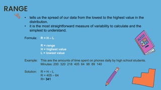
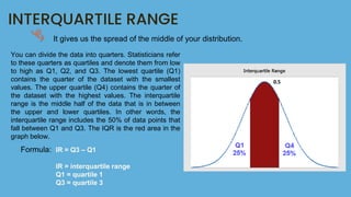
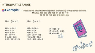
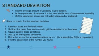
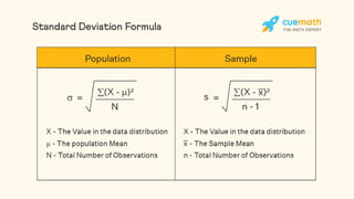
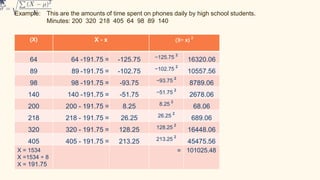
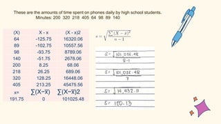
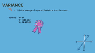
MEASURES OF
VARIABILITY
RANGE, INTERQUARTILE
RANGE, STANDARD
DEVIATION AND VARIANCE
Measure Of Variability
- is a summary statistic that represents the amount of dispersion
in a data set.
- define how far away the data points tend to fall from the
center.
Low Dispersion
High Dispersion
- Indicates that the data points tend to be clustered tightly
around the center.
- Signifies that they tend to fall further away.
Why Measures of Variability Important?
It helps us grasp the likelihood of unusual events.
Example: You are investigating the amounts of time spent on phones daily by different groups of people.
Sample A: high school students Sample B: college students Sample C: adult full-time employees
Let’shaveanexample!
Sample A is ideal because it has low
variability, while sample C is inconsistent
because it ha a high variability.
RANGE
• tells us the spread of our data from the lowest to the highest value in the
distribution.
• it is the most straightforward measure of variability to calculate and the
simplest to understand.
Formula: R = H – L
R = range
H = highest value
L = lowest value
Example: This are the amounts of time spent on phones daily by high school students.
Minutes: 200 320 218 405 64 98 89 140
Solution: R = H – L
R = 405 – 64
R= 341
INTERQUARTILE RANGE
It gives us the spread of the middle of your distribution.
Formula: IR = Q3 – Q1
IR = interquartile range
Q1 = quartile 1
Q3 = quartile 3
You can divide the data into quarters. Statisticians refer
to these quarters as quartiles and denote them from low
to high as Q1, Q2, and Q3. The lowest quartile (Q1)
contains the quarter of the dataset with the smallest
values. The upper quartile (Q4) contains the quarter of
the dataset with the highest values. The interquartile
range is the middle half of the data that is in between
the upper and lower quartiles. In other words, the
interquartile range includes the 50% of data points that
fall between Q1 and Q3. The IQR is the red area in the
graph below.
Example:
INTERQUARTILE RANGE
These are the amounts of time spent on phones daily by high school students.
Minutes: 200 320 218 405 64 98 89 140
64 89 98 140 200 218 320 405
Qk =
𝑘
4
𝑛 + 1
Q1 = ¼ (8+1)
Q1 = ¼ (9)
Q1 = 2.25th
98 – 89 = 9
9 x .25 = 2.25
2.25 + 89 = 91.25
Qk =
𝑘
4
𝑛 + 1
Q3 = ¾ (8+1)
Q3 = ¾ (9)
Q3 = 6.75th
320 – 218 = 102
102 x .75 = 76.5
76.5 + 218 = 294.5.
IR = Q3 – Q1
IR = 294.5 - 91.25
IR = 203.25
STANDARD DEVIATION
• It is the average amount of variability in your dataset.
• is the square root of variance. It is the most stable form of measures of variability.
• (SD) is used when scores are not widely dispersed or scattered.
Steps on how to find the standard deviation:
1. List each score and find their mean.
2. Subtract the mean from each score to get the deviation from the mean.
3. Square each of these deviations.
4. Add up all the squared deviations.
5. Divide the sum of the squared deviations by n – 1 (for a sample) or N (for a population)
6. Find the square root of the number you found.
Example: This are the amounts of time spent on phones daily by high school students.
Minutes: 200 320 218 405 64 98 89 140
(X) X - x (X− x)
𝟐
64 64 -191.75 = -125.75 −125.75
𝟐
16320.06
89 89 -191.75 = -102.75 −102.75
𝟐
10557.56
98 98 -191.75 = -93.75 −93.75
𝟐
8789.06
140 140 -191.75 = -51.75 −51.75
𝟐
2678.06
200 200 - 191.75 = 8.25 8.25
𝟐
68.06
218 218 - 191.75 = 26.25 26.25
𝟐
689.06
320 320 - 191.75 = 128.25 128.25
𝟐
16448.06
405 405 - 191.75 = 213.25 213.25
𝟐
45475.56
X = 1534
X =1534 ÷ 8
X = 191.75
= 101025.48
These are the amounts of time spent on phones daily by high school students.
Minutes: 200 320 218 405 64 98 89 140
(X) X - x (X - x)2
64 -125.75 16320.06
89 -102.75 10557.56
98 -93.75 8789.06
140 -51.75 2678.06
200 8.25 68.06
218 26.25 689.06
320 128.25 16448.06
405 213.25 45475.56
x= ∑(X−x
̅ ) ∑(X−x
̅ )2
191.75 0 101025.48
VARIANCE
• It is the average of squared deviations from the mean.
Formula: V = 𝑺𝟐
V = (𝟏𝟐𝟎. 𝟏𝟑)𝟐
V = 14, 431.22
Thank you!
Meliza M. Sabado
EU - A

Measure of Variability.pptx

  • 1.
  • 2.
    Measure Of Variability -is a summary statistic that represents the amount of dispersion in a data set. - define how far away the data points tend to fall from the center. Low Dispersion High Dispersion - Indicates that the data points tend to be clustered tightly around the center. - Signifies that they tend to fall further away.
  • 3.
    Why Measures ofVariability Important? It helps us grasp the likelihood of unusual events. Example: You are investigating the amounts of time spent on phones daily by different groups of people. Sample A: high school students Sample B: college students Sample C: adult full-time employees Let’shaveanexample! Sample A is ideal because it has low variability, while sample C is inconsistent because it ha a high variability.
  • 4.
    RANGE • tells usthe spread of our data from the lowest to the highest value in the distribution. • it is the most straightforward measure of variability to calculate and the simplest to understand. Formula: R = H – L R = range H = highest value L = lowest value Example: This are the amounts of time spent on phones daily by high school students. Minutes: 200 320 218 405 64 98 89 140 Solution: R = H – L R = 405 – 64 R= 341
  • 5.
    INTERQUARTILE RANGE It givesus the spread of the middle of your distribution. Formula: IR = Q3 – Q1 IR = interquartile range Q1 = quartile 1 Q3 = quartile 3 You can divide the data into quarters. Statisticians refer to these quarters as quartiles and denote them from low to high as Q1, Q2, and Q3. The lowest quartile (Q1) contains the quarter of the dataset with the smallest values. The upper quartile (Q4) contains the quarter of the dataset with the highest values. The interquartile range is the middle half of the data that is in between the upper and lower quartiles. In other words, the interquartile range includes the 50% of data points that fall between Q1 and Q3. The IQR is the red area in the graph below.
  • 6.
    Example: INTERQUARTILE RANGE These arethe amounts of time spent on phones daily by high school students. Minutes: 200 320 218 405 64 98 89 140 64 89 98 140 200 218 320 405 Qk = 𝑘 4 𝑛 + 1 Q1 = ¼ (8+1) Q1 = ¼ (9) Q1 = 2.25th 98 – 89 = 9 9 x .25 = 2.25 2.25 + 89 = 91.25 Qk = 𝑘 4 𝑛 + 1 Q3 = ¾ (8+1) Q3 = ¾ (9) Q3 = 6.75th 320 – 218 = 102 102 x .75 = 76.5 76.5 + 218 = 294.5. IR = Q3 – Q1 IR = 294.5 - 91.25 IR = 203.25
  • 7.
    STANDARD DEVIATION • Itis the average amount of variability in your dataset. • is the square root of variance. It is the most stable form of measures of variability. • (SD) is used when scores are not widely dispersed or scattered. Steps on how to find the standard deviation: 1. List each score and find their mean. 2. Subtract the mean from each score to get the deviation from the mean. 3. Square each of these deviations. 4. Add up all the squared deviations. 5. Divide the sum of the squared deviations by n – 1 (for a sample) or N (for a population) 6. Find the square root of the number you found.
  • 9.
    Example: This arethe amounts of time spent on phones daily by high school students. Minutes: 200 320 218 405 64 98 89 140 (X) X - x (X− x) 𝟐 64 64 -191.75 = -125.75 −125.75 𝟐 16320.06 89 89 -191.75 = -102.75 −102.75 𝟐 10557.56 98 98 -191.75 = -93.75 −93.75 𝟐 8789.06 140 140 -191.75 = -51.75 −51.75 𝟐 2678.06 200 200 - 191.75 = 8.25 8.25 𝟐 68.06 218 218 - 191.75 = 26.25 26.25 𝟐 689.06 320 320 - 191.75 = 128.25 128.25 𝟐 16448.06 405 405 - 191.75 = 213.25 213.25 𝟐 45475.56 X = 1534 X =1534 ÷ 8 X = 191.75 = 101025.48
  • 10.
    These are theamounts of time spent on phones daily by high school students. Minutes: 200 320 218 405 64 98 89 140 (X) X - x (X - x)2 64 -125.75 16320.06 89 -102.75 10557.56 98 -93.75 8789.06 140 -51.75 2678.06 200 8.25 68.06 218 26.25 689.06 320 128.25 16448.06 405 213.25 45475.56 x= ∑(X−x ̅ ) ∑(X−x ̅ )2 191.75 0 101025.48
  • 11.
    VARIANCE • It isthe average of squared deviations from the mean. Formula: V = 𝑺𝟐 V = (𝟏𝟐𝟎. 𝟏𝟑)𝟐 V = 14, 431.22
  • 12.
    Thank you! Meliza M.Sabado EU - A