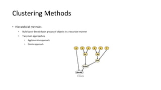
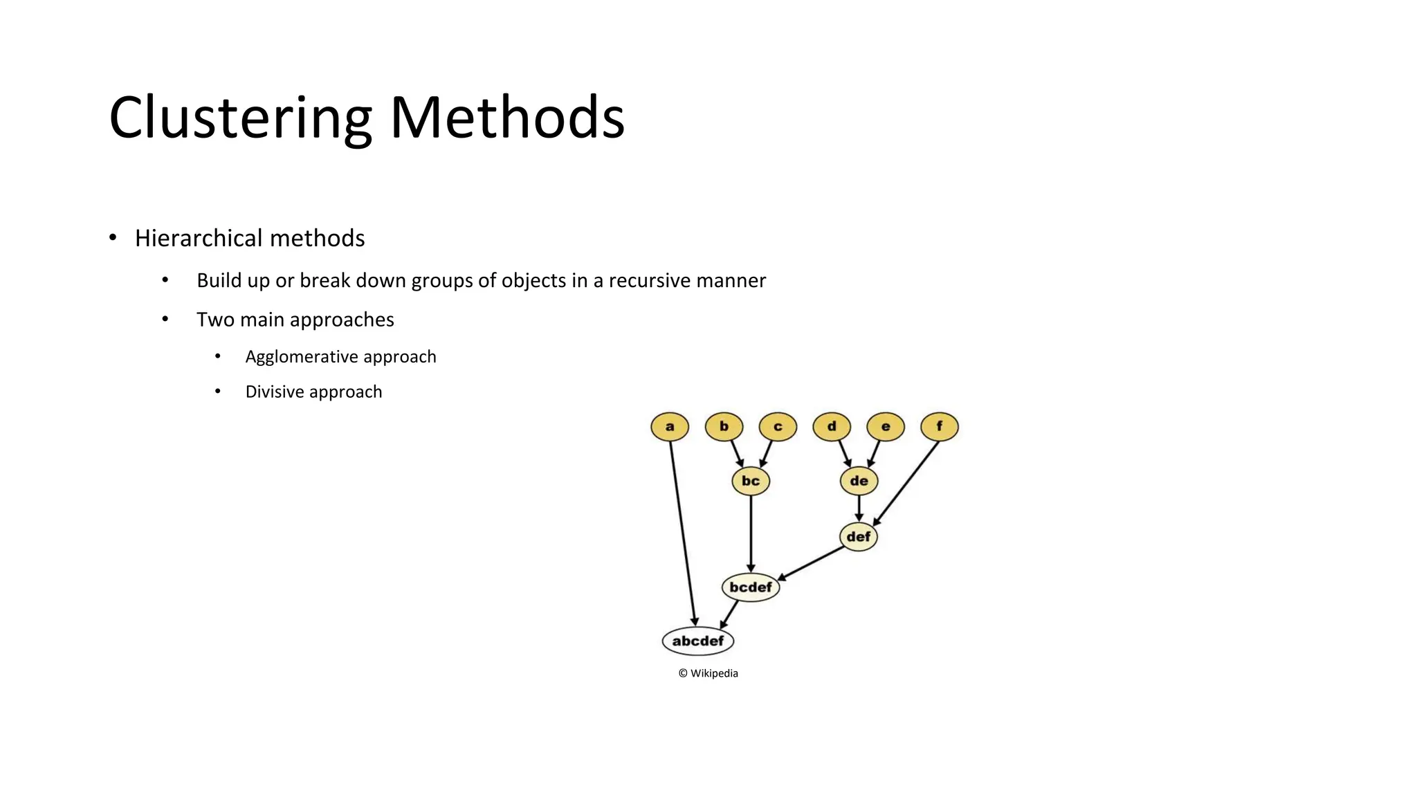
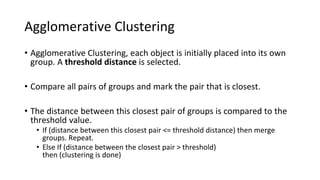
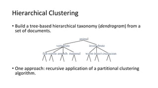
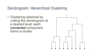
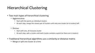
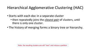
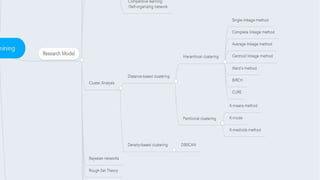
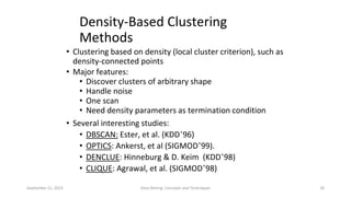
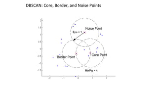
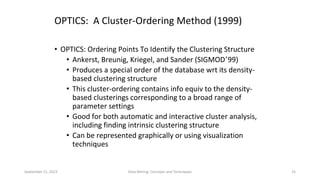
Clustering Methods
• Hierarchical methods
• Build up or break down groups of objects in a recursive manner
• Two main approaches
• Agglomerative approach
• Divisive approach
© Wikipedia
• Hierarchical algorithms
• Bottom-up, agglomerative
• (Top-down, divisive)
Agglomerative Clustering
• Agglomerative Clustering, each object is initially placed into its own
group. A threshold distance is selected.
• Compare all pairs of groups and mark the pair that is closest.
• The distance between this closest pair of groups is compared to the
threshold value.
• If (distance between this closest pair <= threshold distance) then merge
groups. Repeat.
• Else If (distance between the closest pair > threshold)
then (clustering is done)
Hierarchical Clustering
• Build a tree-based hierarchical taxonomy (dendrogram) from a
set of documents.
• One approach: recursive application of a partitional clustering
algorithm.
animal
vertebrate
fish reptile amphib. mammal worm insect crustacean
invertebrate
Ch. 17
Dendrogram: Hierarchical Clustering
• Clustering obtained by
cutting the dendrogram at
a desired level: each
connected component
forms a cluster.
5
Hierarchical Clustering
• Two main types of hierarchical clustering
• Agglomerative:
• Start with the points as individual clusters
• At each step, merge the closest pair of clusters until only one cluster (or k clusters) left
• Divisive:
• Start with one, all-inclusive cluster
• At each step, split a cluster until each cluster contains a point (or there are k clusters)
• Traditional hierarchical algorithms use a similarity or distance matrix
• Merge or split one cluster at a time
Hierarchical Agglomerative Clustering (HAC)
• Starts with each doc in a separate cluster
• then repeatedly joins the closest pair of clusters, until
there is only one cluster.
• The history of merging forms a binary tree or hierarchy.
Sec. 17.1
Note: the resulting clusters are still “hard” and induce a partition
Agglomerative Clustering Algorithm
• More popular hierarchical clustering technique
• Basic algorithm is straightforward
1. Compute the proximity matrix
2. Let each data point be a cluster
3. Repeat
4. Merge the two closest clusters
5. Update the proximity matrix
6. Until only a single cluster remains
• Key operation is the computation of the proximity of two
clusters
• Different approaches to defining the distance between clusters
distinguish the different algorithms
Closest pair of clusters
• Many variants to defining closest pair of clusters
• Single-link
• Similarity of the most cosine-similar (single-link)
• Complete-link
• Similarity of the “furthest” points, the least cosine-similar
• Centroid
• Clusters whose centroids (centers of gravity) are the most cosine-similar
• Average-link
• Average cosine between pairs of elements
Sec. 17.2
What Is A Good Clustering?
• Internal criterion: A good clustering will produce high quality
clusters in which:
• the intra-class (that is, intra-cluster) similarity is high
• the inter-class similarity is low
• The measured quality of a clustering depends on both the
document representation and the similarity measure used
Sec. 16.3
Distance Measures in Algorithmic Methods
Linkage Measures:
• |p − p’ | is the distance between two objects or points, p and p’
• mi is the mean for cluster, Ci
• ni is the number of objects in Ci
Hierarchial Methods
• When an algorithm uses the minimum distance,
dmin(Ci ,Cj) - to measure the distance between clusters
-nearest-neighbor clustering algorithm
• If the clustering process is terminated when the distance between nearest
clusters exceeds a user-defined threshold, it is called a single-linkage
algorithm.
• An agglomerative hierarchical clustering algorithm that uses the minimum
distance measure is also called a minimal spanning tree algorithm.
• When an algorithm uses the maximum distance, dmax(Ci ,Cj), to measure
the distance between clusters, it is sometimes called a farthest-neighbor
clustering algorithm
• If the clustering process is terminated when the maximum distance
between nearest clusters exceeds a user-defined threshold, it is called a
complete-linkage algorithm
BIRCH: Multiphase Hierarchical Clustering
Using Clustering Feature Tree
• Definition:
Balanced Iterative Reducing and Clustering using Hierarchies (BIRCH) is
designed for clustering a large amount of numeric data by integrating
hierarchical clustering (at the initial microclustering stage) and other
clustering methods such as iterative partitioning (at the later
macroclustering stage).
• Advantages:
It overcomes the two difficulties in agglomerative clustering methods:
(1) scalability and
(2) the inability to undo what was done in the previous step
• The clustering feature (CF) of the cluster is a 3-D vector summarizing
information about clusters of objects. It is defined as
CF = (n,LS,SS)
Example of BIRCH
• Clustering feature.
C1=>(2,5),(3,2), and (4,3).
The clustering feature of C1, is
CF1 = (3,(2 + 3 + 4,5 + 2 + 3),(22 + 32 + 42 ,52 + 22 + 32 ) =
(3,(9,10),(29,38)).
Suppose that C1 is disjoint to a second cluster, C2, where
CF2 = (3,(35,36),(417,440)). The clustering feature of a new cluster, C3,
that is formed by merging C1 and C2, is derived by adding CF1 and CF2.
That is, CF3 = (3 + 3,(9 + 35,10 + 36),(29 + 417,38 + 440)) =
(6,(44,46),(446,478))
DBSCAN
• DBSCAN is a density-based algorithm.
• Density = number of points within a specified radius (Eps)
• A point is a core point if it has more than a specified number of
points (MinPts) within Eps
• These are points that are at the interior of a cluster
• A border point has fewer than MinPts within Eps, but is in the
neighborhood of a core point
• A noise point is any point that is not a core point or a border
point.
September 21, 2023 Data Mining: Concepts and Techniques 18
Density-Based Clustering
Methods
• Clustering based on density (local cluster criterion), such as
density-connected points
• Major features:
• Discover clusters of arbitrary shape
• Handle noise
• One scan
• Need density parameters as termination condition
• Several interesting studies:
• DBSCAN: Ester, et al. (KDD’96)
• OPTICS: Ankerst, et al (SIGMOD’99).
• DENCLUE: Hinneburg & D. Keim (KDD’98)
• CLIQUE: Agrawal, et al. (SIGMOD’98)
DBSCAN: Core, Border, and Noise Points
September 21, 2023 Data Mining: Concepts and Techniques 20
DBSCAN: Density Based Spatial Clustering
of Applications with Noise
• Relies on a density-based notion of cluster: A cluster is defined
as a maximal set of density-connected points
• Discovers clusters of arbitrary shape in spatial databases with
noise
Core
Border
Outlier
Eps = 1cm
MinPts = 5
DBSCAN Algorithm
• Eliminate noise points
• Perform clustering on the remaining points
September 21, 2023 Data Mining: Concepts and Techniques 22
DBSCAN: The Algorithm-
Explanation
• Arbitrary select a point p
• Retrieve all points density-reachable from p wrt Eps and
MinPts.
• If p is a core point, a cluster is formed.
• If p is a border point, no points are density-reachable from
p and DBSCAN visits the next point of the database.
• Continue the process until all of the points have been
processed.
DBSCAN: Core, Border and Noise Points
Original Points Point types: core, border
and noise
Eps = 10, MinPts = 4
When DBSCAN Does NOT Work Well
Original Points
(MinPts=4, Eps=9.75).
(MinPts=4, Eps=9.92)
• Varying densities
• High-dimensional data
September 21, 2023 Data Mining: Concepts and Techniques 25
OPTICS: A Cluster-Ordering Method (1999)
• OPTICS: Ordering Points To Identify the Clustering Structure
• Ankerst, Breunig, Kriegel, and Sander (SIGMOD’99)
• Produces a special order of the database wrt its density-
based clustering structure
• This cluster-ordering contains info equiv to the density-
based clusterings corresponding to a broad range of
parameter settings
• Good for both automatic and interactive cluster analysis,
including finding intrinsic clustering structure
• Can be represented graphically or using visualization
techniques
September 21, 2023 Data Mining: Concepts and Techniques 26
OPTICS: Some Extension from DBSCAN
• Index-based:
• k = number of dimensions
• N = 20
• p = 75%
• M = N(1-p) = 5
• Complexity: O(kN2)
• Core Distance
• Reachability Distance
D
p2
MinPts = 5
ε = 3 cm
Max (core-distance (o), d (o, p))
r(p1, o) = 2.8cm. r(p2,o) = 4cm
o
o
p1
September 21, 2023 Data Mining: Concepts and Techniques 27
DENCLUE: using density functions
• DENsity-based CLUstEring by Hinneburg & Keim (KDD’98)
• Major features
• Solid mathematical foundation
• Good for data sets with large amounts of noise
• Allows a compact mathematical description of arbitrarily
shaped clusters in high-dimensional data sets
• Significant faster than existing algorithm (faster than DBSCAN
by a factor of up to 45)
• But needs a large number of parameters
September 21, 2023 Data Mining: Concepts and Techniques 28
• Uses grid cells but only keeps information about grid cells that do
actually contain data points and manages these cells in a tree-
based access structure.
• Influence function: describes the impact of a data point within its
neighborhood.
• Overall density of the data space can be calculated as the sum of
the influence function of all data points.
• Clusters can be determined mathematically by identifying density
attractors.
• Density attractors are local maximal of the overall density function.
Denclue: Technical Essence
September 21, 2023 Data Mining: Concepts and Techniques 29
Grid-Based Clustering Method
• Using multi-resolution grid data structure
• Several interesting methods
• STING (a STatistical INformation Grid approach) by
Wang, Yang and Muntz (1997)
• CLIQUE: Agrawal, et al. (SIGMOD’98)
September 21, 2023 Data Mining: Concepts and Techniques 30
STING: A Statistical Information Grid
Approach
• Wang, Yang and Muntz (VLDB’97)
• The spatial area is divided into rectangular cells
• There are several levels of cells corresponding to different levels
of resolution
STING: A Statistical Information Grid
Approach (2)
• Each cell at a high level is partitioned into a number of smaller cells in the next
lower level
• Statistical info of each cell is calculated and stored beforehand and is used to
answer queries
• Parameters of higher level cells can be easily calculated from parameters of lower
level cell
• count, mean, s, min, max
• type of distribution—normal, uniform, etc.
• Use a top-down approach to answer spatial data queries
• Start from a pre-selected layer—typically with a small number of cells
• For each cell in the current level compute the confidence interval
STING: A Statistical Information Grid
Approach (3)
• Remove the irrelevant cells from further consideration
• When finish examining the current layer, proceed to the next lower level
• Repeat this process until the bottom layer is reached
• Advantages:
• Query-independent, easy to parallelize, incremental update
• O(K), where K is the number of grid cells at the lowest level
• Disadvantages:
• All the cluster boundaries are either horizontal or vertical, and no diagonal boundary is
detected
Data Mining: Concepts and Techniques
CLIQUE (Clustering In QUEst)
• Agrawal, Gehrke, Gunopulos, Raghavan (SIGMOD’98).
• Automatically identifying subspaces of a high dimensional data
space that allow better clustering than original space
• CLIQUE can be considered as both density-based and grid-based
• It partitions each dimension into the same number of equal
length interval
• It partitions an m-dimensional data space into non-overlapping
rectangular units
• A unit is dense if the fraction of total data points contained in
the unit exceeds the input model parameter
• A cluster is a maximal set of connected dense units within a
subspace
Data Mining: Concepts and Techniques
CLIQUE: The Major Steps
• Partition the data space and find the number of points that lie
inside each cell of the partition.
• Identify the subspaces that contain clusters using the Apriori
principle
• Identify clusters:
• Determine dense units in all subspaces of interests
• Determine connected dense units in all subspaces of
interests.
• Generate minimal description for the clusters
• Determine maximal regions that cover a cluster of connected
dense units for each cluster
• Determination of minimal cover for each cluster
Data Mining: Concepts and Techniques
Salary
(10,000)
20 30 40 50 60
age
5
4
3
1
2
6
7
0
20 30 40 50 60
age
5
4
3
1
2
6
7
0
Vacation
(week)
age
Vacation
30 50
τ = 3
Data Mining: Concepts and Techniques
Strength and Weakness of CLIQUE
• Strength
• It automatically finds subspaces of the highest
dimensionality such that high density clusters exist in those
subspaces
• It is insensitive to the order of records in input and does
not presume some canonical data distribution
• It scales linearly with the size of input and has good
scalability as the number of dimensions in the data
increases
• Weakness
• The accuracy of the clustering result may be degraded at
the expense of simplicity of the method
September 21, 2023 Data Mining: Concepts and Techniques 39
What Is Outlier Discovery?
• What are outliers?
• The set of objects are considerably dissimilar from the
remainder of the data
• Example: Sports: Michael Jordon, Wayne Gretzky, ...
• Problem
• Find top n outlier points
• Applications:
• Credit card fraud detection
• Telecom fraud detection
• Customer segmentation
• Medical analysis
September 21, 2023 Data Mining: Concepts and Techniques 40
Outlier Discovery:
Statistical
Approaches
●Assume a model underlying distribution that generates data
set (e.g. normal distribution)
• Use discordancy tests depending on
• data distribution
• distribution parameter (e.g., mean, variance)
• number of expected outliers
• Drawbacks
• most tests are for single attribute
• In many cases, data distribution may not be known
Outlier Discovery: Distance-
Based Approach
• Introduced to counter the main limitations imposed by
statistical methods
• We need multi-dimensional analysis without knowing data
distribution.
• Distance-based outlier: A DB(p, D)-outlier is an object O in a
dataset T such that at least a fraction p of the objects in T lies
at a distance greater than D from O
• Algorithms for mining distance-based outliers
• Index-based algorithm
• Nested-loop algorithm
• Cell-based algorithm
September 21, 2023 Data Mining: Concepts and Techniques 42
Outlier Discovery: Deviation-
Based Approach
• Identifies outliers by examining the main characteristics of
objects in a group
• Objects that “deviate” from this description are considered
outliers
• sequential exception technique
• simulates the way in which humans can distinguish
unusual objects from among a series of supposedly like
objects
• OLAP data cube technique
• uses data cubes to identify regions of anomalies in large
multidimensional data

3b318431-df9f-4a2c-9909-61ecb6af8444.pptx

  • 1.
    Clustering Methods • Hierarchicalmethods • Build up or break down groups of objects in a recursive manner • Two main approaches • Agglomerative approach • Divisive approach © Wikipedia
  • 2.
    • Hierarchical algorithms •Bottom-up, agglomerative • (Top-down, divisive)
  • 3.
    Agglomerative Clustering • AgglomerativeClustering, each object is initially placed into its own group. A threshold distance is selected. • Compare all pairs of groups and mark the pair that is closest. • The distance between this closest pair of groups is compared to the threshold value. • If (distance between this closest pair <= threshold distance) then merge groups. Repeat. • Else If (distance between the closest pair > threshold) then (clustering is done)
  • 4.
    Hierarchical Clustering • Builda tree-based hierarchical taxonomy (dendrogram) from a set of documents. • One approach: recursive application of a partitional clustering algorithm. animal vertebrate fish reptile amphib. mammal worm insect crustacean invertebrate Ch. 17
  • 5.
    Dendrogram: Hierarchical Clustering •Clustering obtained by cutting the dendrogram at a desired level: each connected component forms a cluster. 5
  • 6.
    Hierarchical Clustering • Twomain types of hierarchical clustering • Agglomerative: • Start with the points as individual clusters • At each step, merge the closest pair of clusters until only one cluster (or k clusters) left • Divisive: • Start with one, all-inclusive cluster • At each step, split a cluster until each cluster contains a point (or there are k clusters) • Traditional hierarchical algorithms use a similarity or distance matrix • Merge or split one cluster at a time
  • 7.
    Hierarchical Agglomerative Clustering(HAC) • Starts with each doc in a separate cluster • then repeatedly joins the closest pair of clusters, until there is only one cluster. • The history of merging forms a binary tree or hierarchy. Sec. 17.1 Note: the resulting clusters are still “hard” and induce a partition
  • 8.
    Agglomerative Clustering Algorithm •More popular hierarchical clustering technique • Basic algorithm is straightforward 1. Compute the proximity matrix 2. Let each data point be a cluster 3. Repeat 4. Merge the two closest clusters 5. Update the proximity matrix 6. Until only a single cluster remains • Key operation is the computation of the proximity of two clusters • Different approaches to defining the distance between clusters distinguish the different algorithms
  • 9.
    Closest pair ofclusters • Many variants to defining closest pair of clusters • Single-link • Similarity of the most cosine-similar (single-link) • Complete-link • Similarity of the “furthest” points, the least cosine-similar • Centroid • Clusters whose centroids (centers of gravity) are the most cosine-similar • Average-link • Average cosine between pairs of elements Sec. 17.2
  • 10.
    What Is AGood Clustering? • Internal criterion: A good clustering will produce high quality clusters in which: • the intra-class (that is, intra-cluster) similarity is high • the inter-class similarity is low • The measured quality of a clustering depends on both the document representation and the similarity measure used Sec. 16.3
  • 12.
    Distance Measures inAlgorithmic Methods Linkage Measures: • |p − p’ | is the distance between two objects or points, p and p’ • mi is the mean for cluster, Ci • ni is the number of objects in Ci Hierarchial Methods
  • 13.
    • When analgorithm uses the minimum distance, dmin(Ci ,Cj) - to measure the distance between clusters -nearest-neighbor clustering algorithm • If the clustering process is terminated when the distance between nearest clusters exceeds a user-defined threshold, it is called a single-linkage algorithm. • An agglomerative hierarchical clustering algorithm that uses the minimum distance measure is also called a minimal spanning tree algorithm. • When an algorithm uses the maximum distance, dmax(Ci ,Cj), to measure the distance between clusters, it is sometimes called a farthest-neighbor clustering algorithm • If the clustering process is terminated when the maximum distance between nearest clusters exceeds a user-defined threshold, it is called a complete-linkage algorithm
  • 14.
    BIRCH: Multiphase HierarchicalClustering Using Clustering Feature Tree • Definition: Balanced Iterative Reducing and Clustering using Hierarchies (BIRCH) is designed for clustering a large amount of numeric data by integrating hierarchical clustering (at the initial microclustering stage) and other clustering methods such as iterative partitioning (at the later macroclustering stage). • Advantages: It overcomes the two difficulties in agglomerative clustering methods: (1) scalability and (2) the inability to undo what was done in the previous step
  • 15.
    • The clusteringfeature (CF) of the cluster is a 3-D vector summarizing information about clusters of objects. It is defined as CF = (n,LS,SS)
  • 16.
    Example of BIRCH •Clustering feature. C1=>(2,5),(3,2), and (4,3). The clustering feature of C1, is CF1 = (3,(2 + 3 + 4,5 + 2 + 3),(22 + 32 + 42 ,52 + 22 + 32 ) = (3,(9,10),(29,38)). Suppose that C1 is disjoint to a second cluster, C2, where CF2 = (3,(35,36),(417,440)). The clustering feature of a new cluster, C3, that is formed by merging C1 and C2, is derived by adding CF1 and CF2. That is, CF3 = (3 + 3,(9 + 35,10 + 36),(29 + 417,38 + 440)) = (6,(44,46),(446,478))
  • 17.
    DBSCAN • DBSCAN isa density-based algorithm. • Density = number of points within a specified radius (Eps) • A point is a core point if it has more than a specified number of points (MinPts) within Eps • These are points that are at the interior of a cluster • A border point has fewer than MinPts within Eps, but is in the neighborhood of a core point • A noise point is any point that is not a core point or a border point.
  • 18.
    September 21, 2023Data Mining: Concepts and Techniques 18 Density-Based Clustering Methods • Clustering based on density (local cluster criterion), such as density-connected points • Major features: • Discover clusters of arbitrary shape • Handle noise • One scan • Need density parameters as termination condition • Several interesting studies: • DBSCAN: Ester, et al. (KDD’96) • OPTICS: Ankerst, et al (SIGMOD’99). • DENCLUE: Hinneburg & D. Keim (KDD’98) • CLIQUE: Agrawal, et al. (SIGMOD’98)
  • 19.
    DBSCAN: Core, Border,and Noise Points
  • 20.
    September 21, 2023Data Mining: Concepts and Techniques 20 DBSCAN: Density Based Spatial Clustering of Applications with Noise • Relies on a density-based notion of cluster: A cluster is defined as a maximal set of density-connected points • Discovers clusters of arbitrary shape in spatial databases with noise Core Border Outlier Eps = 1cm MinPts = 5
  • 21.
    DBSCAN Algorithm • Eliminatenoise points • Perform clustering on the remaining points
  • 22.
    September 21, 2023Data Mining: Concepts and Techniques 22 DBSCAN: The Algorithm- Explanation • Arbitrary select a point p • Retrieve all points density-reachable from p wrt Eps and MinPts. • If p is a core point, a cluster is formed. • If p is a border point, no points are density-reachable from p and DBSCAN visits the next point of the database. • Continue the process until all of the points have been processed.
  • 23.
    DBSCAN: Core, Borderand Noise Points Original Points Point types: core, border and noise Eps = 10, MinPts = 4
  • 24.
    When DBSCAN DoesNOT Work Well Original Points (MinPts=4, Eps=9.75). (MinPts=4, Eps=9.92) • Varying densities • High-dimensional data
  • 25.
    September 21, 2023Data Mining: Concepts and Techniques 25 OPTICS: A Cluster-Ordering Method (1999) • OPTICS: Ordering Points To Identify the Clustering Structure • Ankerst, Breunig, Kriegel, and Sander (SIGMOD’99) • Produces a special order of the database wrt its density- based clustering structure • This cluster-ordering contains info equiv to the density- based clusterings corresponding to a broad range of parameter settings • Good for both automatic and interactive cluster analysis, including finding intrinsic clustering structure • Can be represented graphically or using visualization techniques
  • 26.
    September 21, 2023Data Mining: Concepts and Techniques 26 OPTICS: Some Extension from DBSCAN • Index-based: • k = number of dimensions • N = 20 • p = 75% • M = N(1-p) = 5 • Complexity: O(kN2) • Core Distance • Reachability Distance D p2 MinPts = 5 ε = 3 cm Max (core-distance (o), d (o, p)) r(p1, o) = 2.8cm. r(p2,o) = 4cm o o p1
  • 27.
    September 21, 2023Data Mining: Concepts and Techniques 27 DENCLUE: using density functions • DENsity-based CLUstEring by Hinneburg & Keim (KDD’98) • Major features • Solid mathematical foundation • Good for data sets with large amounts of noise • Allows a compact mathematical description of arbitrarily shaped clusters in high-dimensional data sets • Significant faster than existing algorithm (faster than DBSCAN by a factor of up to 45) • But needs a large number of parameters
  • 28.
    September 21, 2023Data Mining: Concepts and Techniques 28 • Uses grid cells but only keeps information about grid cells that do actually contain data points and manages these cells in a tree- based access structure. • Influence function: describes the impact of a data point within its neighborhood. • Overall density of the data space can be calculated as the sum of the influence function of all data points. • Clusters can be determined mathematically by identifying density attractors. • Density attractors are local maximal of the overall density function. Denclue: Technical Essence
  • 29.
    September 21, 2023Data Mining: Concepts and Techniques 29 Grid-Based Clustering Method • Using multi-resolution grid data structure • Several interesting methods • STING (a STatistical INformation Grid approach) by Wang, Yang and Muntz (1997) • CLIQUE: Agrawal, et al. (SIGMOD’98)
  • 30.
    September 21, 2023Data Mining: Concepts and Techniques 30 STING: A Statistical Information Grid Approach • Wang, Yang and Muntz (VLDB’97) • The spatial area is divided into rectangular cells • There are several levels of cells corresponding to different levels of resolution
  • 32.
    STING: A StatisticalInformation Grid Approach (2) • Each cell at a high level is partitioned into a number of smaller cells in the next lower level • Statistical info of each cell is calculated and stored beforehand and is used to answer queries • Parameters of higher level cells can be easily calculated from parameters of lower level cell • count, mean, s, min, max • type of distribution—normal, uniform, etc. • Use a top-down approach to answer spatial data queries • Start from a pre-selected layer—typically with a small number of cells • For each cell in the current level compute the confidence interval
  • 33.
    STING: A StatisticalInformation Grid Approach (3) • Remove the irrelevant cells from further consideration • When finish examining the current layer, proceed to the next lower level • Repeat this process until the bottom layer is reached • Advantages: • Query-independent, easy to parallelize, incremental update • O(K), where K is the number of grid cells at the lowest level • Disadvantages: • All the cluster boundaries are either horizontal or vertical, and no diagonal boundary is detected
  • 34.
    Data Mining: Conceptsand Techniques CLIQUE (Clustering In QUEst) • Agrawal, Gehrke, Gunopulos, Raghavan (SIGMOD’98). • Automatically identifying subspaces of a high dimensional data space that allow better clustering than original space • CLIQUE can be considered as both density-based and grid-based • It partitions each dimension into the same number of equal length interval • It partitions an m-dimensional data space into non-overlapping rectangular units • A unit is dense if the fraction of total data points contained in the unit exceeds the input model parameter • A cluster is a maximal set of connected dense units within a subspace
  • 35.
    Data Mining: Conceptsand Techniques CLIQUE: The Major Steps • Partition the data space and find the number of points that lie inside each cell of the partition. • Identify the subspaces that contain clusters using the Apriori principle • Identify clusters: • Determine dense units in all subspaces of interests • Determine connected dense units in all subspaces of interests. • Generate minimal description for the clusters • Determine maximal regions that cover a cluster of connected dense units for each cluster • Determination of minimal cover for each cluster
  • 36.
    Data Mining: Conceptsand Techniques Salary (10,000) 20 30 40 50 60 age 5 4 3 1 2 6 7 0 20 30 40 50 60 age 5 4 3 1 2 6 7 0 Vacation (week) age Vacation 30 50 τ = 3
  • 38.
    Data Mining: Conceptsand Techniques Strength and Weakness of CLIQUE • Strength • It automatically finds subspaces of the highest dimensionality such that high density clusters exist in those subspaces • It is insensitive to the order of records in input and does not presume some canonical data distribution • It scales linearly with the size of input and has good scalability as the number of dimensions in the data increases • Weakness • The accuracy of the clustering result may be degraded at the expense of simplicity of the method
  • 39.
    September 21, 2023Data Mining: Concepts and Techniques 39 What Is Outlier Discovery? • What are outliers? • The set of objects are considerably dissimilar from the remainder of the data • Example: Sports: Michael Jordon, Wayne Gretzky, ... • Problem • Find top n outlier points • Applications: • Credit card fraud detection • Telecom fraud detection • Customer segmentation • Medical analysis
  • 40.
    September 21, 2023Data Mining: Concepts and Techniques 40 Outlier Discovery: Statistical Approaches ●Assume a model underlying distribution that generates data set (e.g. normal distribution) • Use discordancy tests depending on • data distribution • distribution parameter (e.g., mean, variance) • number of expected outliers • Drawbacks • most tests are for single attribute • In many cases, data distribution may not be known
  • 41.
    Outlier Discovery: Distance- BasedApproach • Introduced to counter the main limitations imposed by statistical methods • We need multi-dimensional analysis without knowing data distribution. • Distance-based outlier: A DB(p, D)-outlier is an object O in a dataset T such that at least a fraction p of the objects in T lies at a distance greater than D from O • Algorithms for mining distance-based outliers • Index-based algorithm • Nested-loop algorithm • Cell-based algorithm
  • 42.
    September 21, 2023Data Mining: Concepts and Techniques 42 Outlier Discovery: Deviation- Based Approach • Identifies outliers by examining the main characteristics of objects in a group • Objects that “deviate” from this description are considered outliers • sequential exception technique • simulates the way in which humans can distinguish unusual objects from among a series of supposedly like objects • OLAP data cube technique • uses data cubes to identify regions of anomalies in large multidimensional data