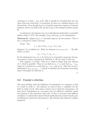
This document discusses sequences and series of numbers. It begins by introducing sequences and the concept of convergence for sequences. A sequence converges to a limit L if, given any positive number ε, there exists an N such that the terms an of the sequence satisfy |L - an| < ε for all n > N. It then proves some basic properties of convergence, including that a convergent sequence must be bounded, and that limits are preserved under operations. Cauchy's criterion for convergence is introduced - a sequence is Cauchy if given any ε, there exists an N such that |am - an| < ε for all m, n > N. Every convergent sequence is Cauchy, and C

1. 2 Sequences and Series
In this chapter we will study two related questions. Given an infinite collec-
tion X of numbers, which can be taken to be rational, real or complex, the
first question is to know if there is a limit point to which the elements of X
congregate (converge). The second question is to know if one can add up all
the numbers in X.
Even though we will be mainly thinking of Q, R or C, many things will
go through for numbers in any field K with an absolute value | . | satisfying
|0| = 0, |x| > 0 if x ̸= 0, |xy| = |x| · |y|, and the triangle inequality |x + y| ≤
|x| + |y|.
A necessary thing to hold for convergence is the Cauchy condition, which
is also sufficient if we work with R or C, but not Q. What we mean by this
remark is that a Cauchy sequence of rational numbers will have a limit L
in R, but L need not be rational. One can enlarge Q to have this criterion
work, i.e., adjoin to Q limits of Cauchy sequences of rational numbers, in
which case one gets yet another construction of R. This aspect is discussed
in section 2.3, which one can skip at a first reading.
The last three sections deal with the second question, and we will derive
various tests for absolute convergence. Sometimes, however, a series might
converge though not absolutely. A basic example of this phenomenon is given
by the Leibniz series
1 1 1 1 1 π
1− + − + − + ... = .
3 5 7 9 11 4
But the series on the left is not absolutely convergent, i.e., the series 1 + 1 +
3
1
5
+ . . . diverges.
2.1 Convergence of sequences
Let K denote either Q or R or C. When we say a number, or a scalar, we
will mean an element of K. But by a positive number we will mean a positive
real number. (One could restrict to positive rational numbers instead, and it
will work just as well to use this subset.)
By a sequence, or more properly an infinite sequence, we will mean a
collection of numbers
a1 , a2 , a3 , . . . , an , an+1 , . . . ,
1

2. which is indexed by the set N of natural numbers. We will often denote it
simply as {an }.
1
A simple example to keep in mind is given by an = n , which appears to
decrease towards zero as n gets larger and larger. In this case we would like
to have 0 declared as the limit of the sequence.
It should be noted that if we are given a collection of numbers indexed by
any countably infinite set, we can reindex it by N and apply all our results
below to it. For example, given M > 0 and {cn | n > −M }, we can renumber
it by putting an = cn+M and get a sequence indexed by N.
We will say that a sequence {an } converges to a limit L in K iff for
every positive number ϵ there exists an index N such that
(2.1.1) n > N =⇒ |L − an | < ϵ.
It is very important to note that we have to check the condition above for
every positive ϵ. Clearly, if (2.2.1) holds for N , it also holds for any N ′ > N .
When {an } does converge to a limit L, we will write
an → L or lim an = L.
n→∞
When we write n → ∞, we do not necessarily mean that there is a number
called ∞, which we have certainly not defined; we mean only that n becomes
arbitrarily large. In other words we want to know what happens to an when
n is larger than any number one can think of.
1
Let us quickly prove that lim is 0, as expected. For any positive number
n→∞ n
1
ϵ, we can find a rational number N such that 0 < N < ϵ. Indeed, by the
property R4 of R (see section 1.0), we can find a rational number q with
0 < q < ϵ, and since q s a positive rational number, we can find an N > 0
1
such that N < q. So for every n > N , we have
1 1 1
|0 − | = < < ϵ,
n n N
1
proving that n
does converge to 0.
When a sequence does not converge to any number L, we will say that it
diverges. A simple example is given by the sequence {1, −1, 1, −1, 1, −1, . . .}.
Given any ϵ < 1, we will be unable to find an N for which (2.1.1) holds for
any L. This is so because for any N {aN +1 , aN +2 } = {1, −1}, and (for any
2

3. L) at least one of them will be at a distance > 1 from L; to see this use the
triangle inequality |L − aN +1 | ≤ |L − aN +2 | + |aN +2 − aN +1 |, together with
|aN +2 − aN +1 | = 2.
Any sequence which converges (to some limit) will be called a convergent
sequence, and one that does not converge will be called a divergent sequence.
Proposition 2.1.2
(i) If {an } is a convergent sequence with limit L, then for any scalar c, the
sequence {can } is convergent with limit cL;
(ii) If {an }, {bn } are convergent sequences with respective limits L1 , L2 ,
then their sum {an + bn } and their product {an bn } are convergent with
respective limits L1 + L2 and L1 L2 .
The proof is a simple application of the properties of absolute values. To
illustrate, let us prove the assertion about the sum sequence {an + bn }. Pick
any ϵ > 0. Since an → L1 and bn → L2 , we can find N > 0 such that
ϵ ϵ
n > N =⇒ |L1 − an | < , |L2 − bn | < .
2 2
Using the triangle inequality we then have, for all n > N ,
ϵ ϵ
|(L1 + L2 ) − (an + bn )| ≤ |L1 − an | + |L2 − bn | < + = ϵ.
2 2
Hence an + bn → L1 + L2 .
Corollary 2.1.3 Let {zn = xn + iyn } be a sequence of complex numbers,
with xn , yn real for each n. Then {zn } converges iff the real sequences {xn }
and {yn } are both convergent.
Proof. Suppose {xn }, {yn } are both convergent, with respective limits
u, v. We claim that {zn } then converges to w = u + iv. Indeed, by the
Proposition above, {iyn } is convergent with limit iv, and so is {xn + iyn },
with limit w. Conversely, suppose that {zn } converges, say to w. We may
write w as u + iv, with u, v real. For any complex number z = x + iy, |x|
√
and |y| are both bounded above by x2 + y 2 , i.e., by |z|. Since w − zn =
(u − xn ) + i(v − yn ), we get
|u − xn | ≤ |w − zn | and |v − yn | ≤ |w − zn |.
3

4. For any ϵ > 0, pick N > 0 such that for all n > N , |w − zn | is < ϵ. Then
we also have |u − xn | < ϵ and |v − yn | is < ϵ for all n > N , establishing the
convergence of {xn } and {yn } with respective limits u and v.
Thanks to this Corollary, the study of sequences of complex numbers can
be reduced to that of real numbers.
A sequence {an } is bounded iff there is a positive number M such that
|an | ≤ M for all n.
Lemma 2.1.4 If a sequence {an } converges, then it must be bounded.
Proof Let L be the limit of {an }. Fix any positive number ϵ. Then by
definition, there exists an N > 0 such that for all n > N , |L − an | is < ϵ. By
the triangle inequality,
|an | ≤ |an − L| + |L|.
So if we set
M = max{a1 , a2 , . . . , aN , L + ϵ},
then every |an | is bounded by M .
The converse of this Lemma is not true: Remember that the sequence
{1, −1, 1, −1, . . .} has not limit, but it is bounded in absolute value by 1.
For any real number x and consider the power sequence {xn }. When x = 1
(resp. 0), we get the stationary sequence {1, 1, 1, . . .} (resp. {0, 0, 0, . . .}),
which is obviously convergent with limit 1 (resp. 0). When x = −1, we get
{−1, 1, −1, . . .}, which is divergent, as we saw above. Applying the following
Lemma we see that this sequence is unbounded when |x| > 1, hence divergent,
and that it converges to zero when |x| < 1.
Lemma 2.1.5 Let y be a positive real number. Then {y n } is unbounded if
y > 1, while
lim y n = 0 if y < 1.
n→∞
Proof of Lemma. Suppose y > 1. Write y = 1 + t with t > 0. Then by
the binomial theorem (which can be proved by induction),
∑ (n)
n
n n
y = (1 + t) = tk ,
k=1
k
4

5. which is ≥ 1 + nt. Since 1 + nt is unbounded, i.e, larger than any number
for a big enough n, y n is also unbounded.
Now let y < 1. Then y −1 is > 1 and hence {y −n } is unbounded. This
implies that, for any ϵ > 0, y n is < ϵ for large enough n. Hence the sequence
y n converges to 0.
A sequence of real (or rational) numbers an is said to be monotone in-
creasing, resp. monotone decreasing, iff for all n, an ≤ an+1 , resp. an ≥ an+1 ;
it is said to be simply monotone if it is either monotone increasing or mono-
tone decreasing.
Theorem A If {an } is a bounded, monotone sequence of real numbers,
then it converges in R, in fact to the supremum, resp. infimum, when {an }
is increasing, resp. decreasing.
Proof. Suppose {an } is monotone increasing. Since R is a complete
ordered field, every bounded subset has a least upper bound. Since {an } is
bounded, we may look at its supremum M , say. We claim that an → M .
Suppose not. Then there exists an ϵ > 0 such that for every N > 0, there
exists an n > N such that |M − an | ≥ ϵ. Since the sequence is monotone
increasing, we then have
ϵ
|an | < M − , ∀n ≥ 1.
2
Then M − 2 is an upper bound for {an }, and so M could not be the least
ϵ
upper bound. Contradiction! So M must be the limit of the sequence.
Now suppose {an } is monotone decreasing. Then the sequence {−an } is
monotone increasing, and it is bounded because {an } is. So {−an } converges;
then so does {an }.
Here is an example. Define a sequence {an } by putting
1 1 1
an = 1 + + + ... + .
1! 2! (n − 1)!
It is not hard to see that this sequence is bounded. Try to give a proof.
(In fact one can show that it is bounded by 3, but we do not need the best
possible bound at this point.) Clearly, an+1 > an , so the sequence is also
monotone increasing. So we may apply the Theorem and conclude that it
5

6. converges to a limit e, say, in R. But it should be remarked that one can
show with more work that e is irrational. So there is a valuable lesson to be
learned here. Even though {an } is a bounded, monotone sequence of rational
numbers, there is no limit in Q; one has to go to the enlarged number system
R.
A subsequence of a sequence {an } is a subcollection indexed by a countably
infinite subset J of N. For example, {a2n } and {a2n+1 } are subsequences.
Theorem B Suppose {an } is a bounded sequence of real numbers. Then it
has a subsequence which converges.
Proof. Put
J = {m ∈ N | an ≤ am , ∀ n ≥ m}.
Suppose J is an infinite set. Write its elements as m1 , m2 , m3 , . . .. By defi-
nition, we have
am1 ≥ am2 ≥ am3 ≥ . . . .
So the subsequence {am | m ∈ J} (of {an }) is a bounded, monotone decreas-
ing sequence, hence convergent by Theorem A. We are done in this case.
Now suppose J is finite. Pick an n1 which is larger than any element
of J, which is possible. Then we can find an n2 > n1 such that an1 < an2 .
Again we can find an n3 such that an2 < an3 , and so on. This way we get a
subsequence {an1 , an2 , an3 , . . .} which is bounded and monotone increasing,
hence convergent by Theorem A.
2.2 Cauchy’s criterion
The main problem with the definition of convergence of a sequence is that
it is hard to verify it. For instance we need to have a candidate for the
limit to verify (2.1.2). One wants a better way to check for convergence. As
seen above, boundedness is a necessary, but not sufficient, condition, unless
the sequence is also monotone (and real). Is there a necessary and sufficent
condition? A nineteenth century French mathematician named Cauchy gave
an affirmative answer for real sequences. His criterion also works for complex
sequences.
6

7. A sequence {an } is said to be a Cauchy sequence iff we can find, every
positive ϵ, an N > 0 such that
(2.2.1) |am − an | < ϵ whenever n, m > N.
This is nice because it does not mention any limit.
Lemma 2.2.2 Every convergent sequence is Cauchy.
Proof. Suppose an → L. Pick any ϵ > 0. Then by definition, we can
find an N > 0 such that, for all n > N , we have
ϵ
|L − an | <
2
Then for n, m > N , the triangle inequality gives
ϵ ϵ
|am − an | ≤ |am − L| + |L − an | < + = ϵ.
2 2
Lemma 2.2.3 A complex sequence {zn = xn + iyn }, with xn , yn real, is
Cauchy iff {xn } and {yn } are Cauchy.
Proof. Suppose {xn }, {yn } are both Cauchy. Pick any ϵ > 0. Then we
can find an N > 0 such that for all m, n > N ,
ϵ ϵ
|xm − xn | < , and |ym − yn | < .
2 2
Since zm − zn is (xm − xn ) + i(ym − yn ) and |i| = 1, , we get by the triangle
inequality,
|zm − zn | ≤ |xm − xn | + |ym − yn | < ϵ.
Conversely, suppose that {zn } is Cauchy. Recall that for any complex number
√
z = x + iy, |x| and |y| are both bounded by ≤ x2 + y 2 , i.e., by |z|. This
immediately implies that {xn } and {yn } are Cauchy.
Here comes the beautiful result of Cauchy:
Theorem C Every Cauchy sequence of real (resp. complex) numbers con-
verges in R (resp. C).
Proof. By Corollary 2.1.3, a sequence {zn = xn + iyn } of complex
numbers is convergent iff the real sequences {xn } and {yn } are convergent.
7

8. By Lemma 2.2.3, {zn } is Cauchy iff {xn }, {yn } are. So it suffices to prove
Theorem C for real Cauchy sequences {an }.
First note that such a sequence must be bounded. Indeed, fix an ϵ > 0 and
find an N > 0 for which (2.2.1) holds. Then for all n > N , an lies between
aN +1 − ϵ and aN +1 + ϵ. Then the set {an | n > N } is bounded. Then so is
the entire sequence because {a1 , . . . , aN } is finite.
Now since {an }is a bounded, real sequence, we can apply Theorem B and
find a subsequence {am1 , am2 , . . .} which converges, say to the limit L. We
claim that the original sequence {an } also converges to L. Indeed, let ϵ be
an arbitrary positive number. Then we can find an N > 0 such that for all
mk , n > N ,
ϵ ϵ
|L − amk | < and |amk − an | < .
2 2
Applying the triangle inequality we get
|L − an | < ϵ, ∀ n > N,
proving the claim.
2.3 Construction of Real Numbers revisited
Given any Cauchy sequence {an } of rational numbers, we may of course
view it as a real sequence and apply Theorem C to deduce that it converges
to a limit L, say. But this L need not be rational. This leads us to wonder
if all the real numbers could be constructed by adjoining limits of Cauchy
sequences of rational numbers. This is essentially correct, and this approach
is quite different from that given in chapter 1. Now let us explain how it is
done.
Let us begin by pretending that we do not know what real numbers are,
but that we know everything about rational numbers.
The first thing to note is that different Cauchy sequences of rational
numbers might have the same limit. For example, the sequences {0, 0, 0, . . .}
and {1, 2 , 1 , . . .} have 0 as their limit. So we define an equivalence between
1
3
any pair of Cauchy sequences {an } and {bn } with an , bn ∈ Q are as follows:
(2.3.1) {an } ∼ {bn } ⇔ lim (an − bn ) = 0.
n→∞
8

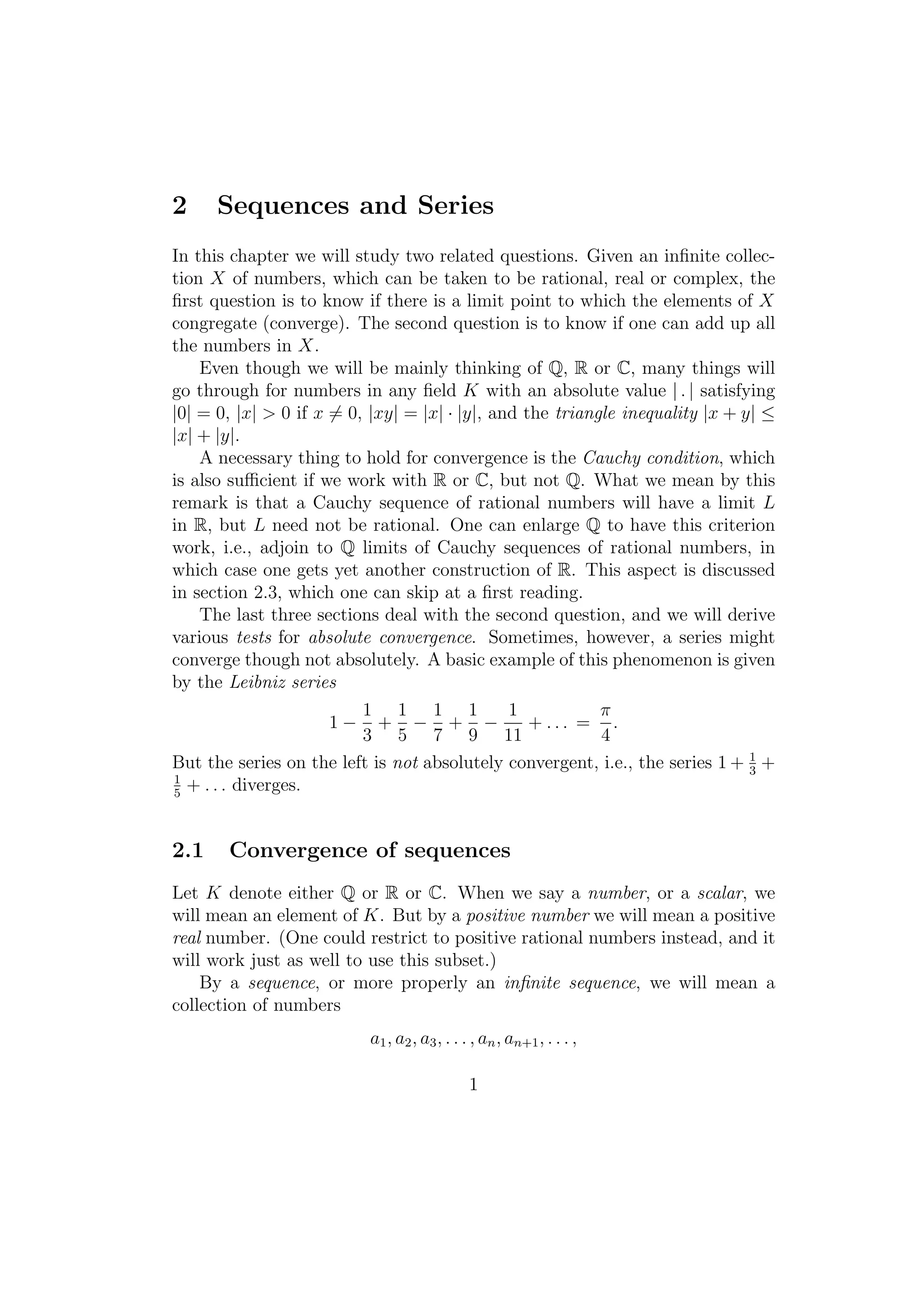
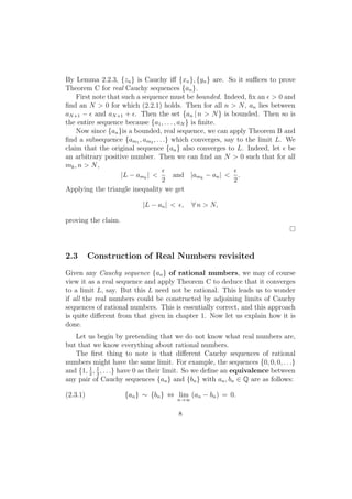
9. It will be left as a good exercise for the students to check that ∼ is indeed
an equivalence relation in the sense of chapter 0.
Denote the equivalence class of any {an } by [an ]. It is not hard to check
that given two classes [an ] and [bn ], they are either the same or disjoint, i.e.,
no rational Cauchy sequence {cn } can belong to two distinct classes.
Define a real number to be an equivalence class [an ] as above. Denote
by R the collection of all real numbers in this sense. We then have a natural,
mapping
Q → R, q → [q, q, q, . . .],
where [q, q, q, . . .] is the class of the stationary sequence {q, q, q, . . .} (which
is evidently Cauchy). This mapping is one-to-one because if q, q ′ are unequal
rational numbers, then {q, q, q, . . .} cannot be equivalent to {q ′ , q ′ , q ′ , . . .}.
Consequently, we have 0 and 1 in R.
We know that the sum and product of Cauchy sequences are again Cauchy.
So we may set
[an ] ± [bn ] = [an ± bn ], and [an ] · [bn ] = [an bn ].
It is immediate that one has commutativity, associativity and distributivity.
It remains to define a multiplicative inverse of a non-zero element ρ of R.
Let {an } be a Cauchy sequence belonging to ρ. Since ρ is non-zero, all but
a finite number of the an must be non-zero. Let {amn } be the subsequence
consisting of all the non-zero terms of {an }. Then this subsequence also
represents ρ, and we may set
ρ−1 = [a−1 ].
mn
Check that this gives a well defined multiplicative inverse.
Now it is more or less obvious that R is a field under these operations,
containing Q as a subfield.
Next comes the notion of positivity. Define a real number ρ to be positive
iff for some Cauchy sequence {an } representing ρ, we can find an N > 0 such
that an is positive for all n > N . Check that this intuitive notion is the right
one.
Armed with this powerful notion, one sees that R becomes an ordered
field. By definition, the ordering on R is compatible with the usual one on
Q.
9

10. Finally, every Cauchy sequence converges in R. This is a nice consequence
of our construction. When ρ is represented by a Cauchy sequence {an }, the
sequence is forced to converge to ρ.
Now we will end this section by discussing how one can mathematically
define real numbers via their decimal expansions, which everyone intu-
itively understands. Here is what one does.
Define a real number to be a pair (m, {an }), where m is an integer and
{an } is a sequence of non-negative integers, with the understanding that an
is not all 9 after some index N . One often writes
∑
∞
(m, {an }) = m + an 10−n .
n=1
∑
r
If we have a rational number of the form m + an , we will identify it with
n=1
(m, {an }) with an = 0 for all n > r.
Define an ordering by setting
(m, {an }) < (k, {bn }) ⇔ m < k or m = k, ∃N s.t. aN < bN , an = bn ∀ n < N.
This leads quickly to the least upper bound property, so we can take the
suprema of bounded sets.
Given any real number ρ = (m, {an }), we will define, for each r ≥ 1, its
truncation at stage r to be
∑
r
ρr = m + an ∈ Q.
n=1
Evidently,
ρ = sup{ρr | r ≥ 1}.
So it is natural to set, for real numbers ρ, ρ′ ,
ρ ± ρ′ = sup{ρr ± ρ′r }
and
ρ · ρ′ = sup{ρk · ρ′k }.
The definition of the multiplicative inverse of a non-zero ρ is left as an exer-
cise.
10

11. 2.4 Infinite series
Given a sequence {an }, we will often want to know if we can sum the terms
of the sequence, denoted
∑
∞
(2.4.1) S = an ,
n=1
and get something meaningful. Such an infinite sum is called an infinite
series.
A natural way to proceed is as follows. We know how to sum, for any
n ≥ 1, the first n terms of the sequence, namely
∑
n
(2.4.2) sn = an .
m=1
This way we get another sequence {sn }, called the sequence of partial sums.
(One calls sn the nth partial sum.) We will say that the original sequence
{an } is summable, or that the infinite series (2.4.1) is convergent, iff the
sequence of partial sums converges.
Let us first look at the example of a geometric series. Fix any real
number x with |x| < 1, and put
an = xn−1 (∀ n ≥ 1),
and
∑
∞
(2.4.3) S = xn−1 = 1 + x + x2 + x3 + . . .
n=1
We claim that
1 − xn
sn = .
1−x
Indeed, we have
(1−x)sn = (1−x)(1+x+x2 +. . .+xn−1 ) = (1−x)+(x−x2 )+. . .+(xn−1 −xn ) = 1−xn ,
proving the claim.
11

12. Now by Lemma 2.1.5 (and the discussion preceding it), we have
xn → 0 since |x| < 1.
Consequently,
1
(2.4.4) S = lim sn = .
n→∞ 1−x
Check that the series is divergent if |x| ≥ 1.
Lemma 2.4.5 If {an }, {bn } are summable sequences, then so is {c1 an +c2 bn }
for any pair of scalars c1 , c2 .
The proof is straight-forward and will be left as an exercise. The reader
should take note, however, that nothing is claimed here about the product
of two sequences.
∑ ∑
We will say that a series an is absolutely convergent if the series |an |
n≥1 n≥1
is convergent. In this case one also says that the sequence {an } is absolutely
summable. This notion is important and makes us want to understand well
the summability of positive sequences, which will be our focus in the next
section. It should be noted however (see section 2.6) that there are summable
sequences, which are not absolutely summable.
One of the most important reasons for studying absolutely summable
sequences is that it allows one to study the product of two sequences. This
is encapsulated in the following Proposition, which we will quote without
proof.
Proposition 2.4.6 Suppose {an }, {bn } are two absolutely summable se-
quences. Consider the sequence {cn } with
∏
cn = ai b j .
i+j=n
Then {cn } is absolutely summable and moreover,
∑
∞ ∑
∞ ∑
∞
cn = an · bn .
n=1 n=1 n=1
12

13. 2.5 Tests for Convergence
We will concentrate mainly on the summability of sequences with non-negative
terms.
The first thing one notices about such a sequence {an } with each an
non-negative, is that
s1 ≤ s2 ≤ . . . ≤ sn ≤ . . . ,
i.e., {sn } is monotone increasing. In view of Theorem A, we then get the
following
Lemma 2.5.1 A sequence of non-negative numbers is summable iff the
associated sequence {sn } of partial sums is bounded.
The first test for convergence is given by the following
Proposition 2.5.2 (Comparison test) Let {an }, {bn } be non-negative
sequences of real numbers, such that
(i) an ≤ bn for all n ≥ 1; and
(ii) The sequence {bn } is summable.
Then {an } is summable.
Proof. Let sn , tn denote the n-th partial sums of {an }, {bn } respectively.
Then we have (for all n)
sn ≤ tn .
Since by hypothesis the sequence {bn } is summable, the sequence {tn } con-
verges. Then the tn , and hence the sn , must be bounded. So the sequence
{an } is summable by Lemma 2.5.1.
Here comes the second test.
Proposition 2.5.4 (Ratio test)) Let {an } be a sequence of non-negative
terms. Suppose the sequence {an+1 /an } of ratios converges to a real number
r.
(i) If r < 1, then {an } is summable;
∑
(ii) If r > 1, then {an } is not summable, i.e., the series an diverges.
n≥1
13

14. It is important to note that this test says nothing when r = 1.
Proof. Suppose r is less than 1. Pick any ϵ > 0 with r + ϵ < 1. Write
t = r + ϵ, so that r < t < 1. Then as {an+1 /an } converges to r, we can find
an N > 0 such that for all n > N , |r − an+1 /an | < ϵ. This implies that
an+1
n>N ⇒ < t.
an
In other words,
aN +2 < aN +1 t, aN +3 < aN +2 t < aN +1 t2 , . . .
We can rewrite it as saying that for all j ≥ 1, we have
aN +j < aN +1 tj−1 ,
so that
∑
∞ ∑
∞
aN +j < aN +1 tj−1 .
j=1 j≥1
∑
This converges by the comparison test, because the geometric series j≥1 tj−1
1
occurring on the right is convergent as t is positive and < 1 (with limit 1−t ).
∑ ∑
Consequently, the (partial) series an , and hence the whole series an ,
n>N n≥1
converges.
When r > 1, one sees easily that the sequence of partial sums is not
bounded, hence divergent.
Given a positive real number x and a positive integer n, there is a unique
positive real number, denoted x1/n , which is an n-th root of x, i.e., (x1/n )n =
x. We will also set 01/n = 0.
Proposition 2.5.5 (Root test) Let {an } be a sequence of non-negative
1/n
real numbers. Suppose the associated root sequence {an } is convergent with
limit R, Then the following hold:
∑
(i) If R < 1, then the series an converges;
n≥1
∑
(ii) If R > 1, then the series an diverges.
n≥1
14

15. Just as in the Ratio test, this test says nothing when R = 1.
Proof. Suppose R < 1. Pick any ϵ > 0 with R + ϵ < 1. Write t = R + ϵ,
1/n
so that R < t < 1. Then as {an } converges to R, we can find an N > 0
1/n
such that for all n > N , |R − an | < ϵ. This implies that
n > N ⇒ an < tn .
Hence ∑ ∑ ∑
an < tn < tn .
n>N n>N n≥1
The (partial) series on the left now converges by the comparison test, because
∑ n
the geometric series n≥1 t occurring on the right ∑ convergent (as t is
is
positive and < 1). Consequently, the complete series an also converges.
n≥1
When R > 1, the sequence of partial sums is not bounded, hence diver-
gent.
2.6 Alternating series
One of the most beautiful formulas in Mathematics is the formula of Leibniz
for π/4 given at the beginning of this chapter. It is one of the glorious
examples of what are known as alternating series, i.e., whose terms alternate
in sign, which converge but not absolutely. Some people use the terminology
conditional convergence for this phenomenon. Leibniz was amazing in that
he not only found a slew of such formulas, he also discovered a theorem which
gives precise conditions on an alternating series to be convergent. Let us now
state and prove it.
Theorem D (Leibniz ) Let {bn } be a sequence of non-negative, mono-
tone decreasing sequence such that
lim bn = 0.
n→∞
Then the alternating series
∑
∞
S = (−1)n+1 bn = b1 − b2 + b3 − b4 + . . .
n=1
15

16. is convergent.
Proof. Put an = (−1)n+1 bn and
sn = a1 + a2 + . . . + an = b1 − b2 + . . . + (−1)n+1 bn .
We have to show that the sequence {sn } of partial sums converges. First
note that for any n ≥ 1,
(2.6.1) s2n = s2n−1 − b2n ≤ s2n−1 ,
since the bj are non-negative. We also have (for all n ≥ 2)
(2.6.2) s2n = s2n−2 + b2n−1 − b2n ≤ s2n−2 ,
and
(2.6.3) s2n−1 = s2n−3 − b2n−2 + b2n−1 ≥ s2n−3 ,
both since the bj are monotone decreasing.
Now let i, j be natural numbers such that i is even and j odd. Then we
may pick an n > 0 such that 2n ≥ i and 2n − 1 ≥ j. Applying (2.6.1), (2.6.2)
and (2.6.3), we deduce that
(2.6.4) si ≤ s2n ≤ s2n−1 ≤ sj .
In particular, si is bounded from above, for any even index i, by s1 = b1 .
Similarly, for any odd index j, sj is bounded from below by s2 = b1 − b2 .
The inequalities given by (2.6.2) and (2.6.3) show that the subsequence
{s2n } is monotone increasing and {s2n−1 } is monotone decreasing. Since the
former is bounded from above, and the latter from below, they both converge,
say to respective limits ℓ and L, i.e., we have
lim s2n = ℓ ≤ L = lim s2n−1 .
n→∞ n→∞
The assertion ℓ ≤ L follows from (2.6.4).
Finally, note that by definition,
s2n − s2n−1 = −b2n .
Since the bn converge to zero as n → ∞, we see that the subsequences {s2n }
and s2n−1 must both converge to the same limit, i.e., ℓ = L. Consequently,
lim sn = L.
n→∞
16

17. Here are some examples of alternating series:
1 1 1
(2.6.5) S1 = 1 − + − + ...
2 3 4
1 1 1
(2.6.6) S2 = 1 − + − + ...
3 5 7
π2 π5 π7
(2.6.7) S3 = π − + − + ...
3! 5! 7!
Clearly, { n } and { 2n−1 } are non-negative, decreasing sequences converging
1 1
to zero. So we may apply Leibniz’s theorem above and conclude that S1 and
S2 converge. Even though we will not evaluate these limits here, let us note
that
π
(2.6.8) S1 = log 2 and S2 = .
4
Let us now turn to (2.6.7). We need to know that
πn π n−1
(2.6.9) ≤
n! (n − 1)!
and that
πn
(2.6.10) → 0 as n → ∞.
n!
Since π is known to be < 4, (2.6.9) is satisfied for all n ≥ 4, and when
we study exponential functions later in the course, we will see the truth of
(2.6.10). So by Leibniz’s theorem, the series starting with n = 4 converges.
So S3 itself converges. The amazing things is that one can show:
S3 = 0.
17