This document is the thesis of Alessandro Adamo submitted for a PhD in Mathematics and Statistics for Computational Sciences. The thesis proposes a new algorithm called LIMAPS (Lipschitzian Mappings for Sparse recovery) for solving underdetermined linear systems based on nonconvex Lipschitzian mappings. Chapter 1 provides theoretical foundations on sparse recovery and compressive sensing. Chapter 2 introduces LIMAPS and its iterative scheme for sparse representation and sparsity minimization. Chapters 3 and 4 apply LIMAPS to face recognition and ECG signal compression respectively, demonstrating its effectiveness on real-world applications.


![Introduction
In recent years, the sparsity concept has attracted considerable attention in areas
of applied mathematics and computer science, especially in signal and image pro-
cessing fields [41, 29, 55]. The general framework of sparse representation is now
a mature concept with solid basis in relevant mathematical fields, such as prob-
ability, geometry of Banach spaces, harmonic analysis, theory of computability,
and information-based complexity. Together with theoretical and practical advance-
ments, also several numeric methods and algorithmic techniques have been devel-
oped in order to capture the complexity and the wide scope that the theory suggests.
All these discoveries explain why sparsity paradigm has progressively interested a
broad spectrum of natural science and engineering applications.
Sparse recovery relays over the fact that many signals can be represented in a
sparse way, using only few nonzero coefficients in a suitable basis or overcomplete
dictionary. The problem can be described as follows. Given a fixed vector s ∈ Rn
and a matrix Φ ∈ Rn×m with m > n, determine the sparsest solution α∗, i.e.
α∗
= argmin
α
||α||0, s.t. Φα = s (BP0)
where || · ||0 is the ℓ0 quasinorm, that represents the number of non-zero entries of
the vector α.
Unfortunately, this problem, also called ℓ0-norm minimization, is not only NP-hard
[85], but but also hard to approximate within an exponential factor of the optimal
solution [87]. Nevertheless, many heuristics for the problem has been obtained and
proposed for many applications. Among them we recall a greedy pursuit technique
that approximates a sparse solutions to an underdetermined linear system of equa-
tions. Successively, several greedy-based extended heuristics that directly attempt
to solve the ℓ0-norm minimization have been proposed, for instance, Matching Pur-
suit (MP) [77], Orthogonal Matching Pursuit (OMP) [91] and Stagewise Orthogonal
Matching Pursuit (StOMP) [45].
xv](https://image.slidesharecdn.com/f546e914-990d-4b7e-af7b-78d9394c1be8-160713201804/85/phd_unimi_R08725-13-320.jpg)
![xvi List of Tables
A second key contribution [31] relaxes the problem by using the ℓ1-norm for
evaluating sparsity and solving the relaxed problem by linear programming. Typical
algorithm in this class of algorithms is Basis Pursuit (BP) [29]
This thesis provides new regularization methods for the sparse representation
problem with application to face recognition and ECG signal compression. The
proposed methods are based on fixed-point iteration scheme which combines non-
convex Lipschitzian-type mappings with canonical orthogonal projectors. The first
are aimed at uniformly enhancing the sparseness level by shrinking effects, the lat-
ter to project back into the feasible space of solutions. In particular the algorithm
LIMAPS (Lipshitzian Mappings for Sparse recovery) is proposed as heuristics for
(BP0). This algorithm is based on a parametric class Gλ of nonlinear mappings
Gλ : {α | s = Φα} → {α | s = Φα}.
First of all, the problem (BP0) is relaxed to the problem
α∗
= argmin
α
||α||<λ>, s.t. Φα = s (REL)
where, for all λ > 0, ||·||<λ> is a suitable pseudonorm such that ||α||0 ≈ ||α||<λ>
for large λ.
The main result we obtain in this part states under reasonable conditions, the
minima of (REL) are asymptotically stable fixed points of Gλ with respect to the
iterative system
αt+1 = Gλ (αt )
Then, the LIMAPS algorithm requires a suitable sequence {λt} with limt→∞ λt = ∞
Roughly speaking, this implies that || · ||<λ> ≈ || · ||0 for large t. LIMAPS imple-
ments the system
αt+1 = Gλ (αt )
for obtaining a sparse solution as t → ∞.
In many applications, it is often required to solve the variant of (BP0) in which
the sparsity level is a given as a constant:
α∗
= argmin
α
||Φα − s||2
2, s.t. ||α||0 ≤ 0 (LS0)
In this thesis we propose a heuristic for (LS0) the algorithm k-LIMAPS . An empir-
ical evidence of convergence of k-LIMAPS to good solutions is discussed.
In the second part of this thesis we study two applications in which sparseness
has been successfully applied in recent areas of the signal and image processing: the
face recognition problem and the ECG signal compression problem.
In the last decades, the face recognition (FR) problem has received increasing
attention. Despite excellent results have been achieved, the existing methods suf-
fer when applied in uncontrolled conditions. Such bottleneck represents a serious
limit for their real applicability. In this work we propose two different algorithms](https://image.slidesharecdn.com/f546e914-990d-4b7e-af7b-78d9394c1be8-160713201804/85/phd_unimi_R08725-14-320.jpg)


![Chapter 1
Sparse Recovery and Compressive Sensing
Abstract Shannon-Nyquist sampling theorem is one of the central principle in
signal processing. To reconstruct without error a signal s(t) with no frequencies
higher than B Hertz by the sampled signal sc(t), it is sufficient a sampling frequency
A > 2B.
In the last few years a further development called compressive sensing has emerged,
showing that a signal can be reconstructed from far fewer measurements than what
is usually considered necessary, provided that it admits a sparse representation.
In this chapter we provide a brief introduction of the basic theory underlying com-
pressive sensing and discuss some methods to recovery a sparse vector in efficient
way.
1.1 Introduction
Compressive sensing (CS) has emerged as a new framework for signal acquisition
and sensor design [47, 28]. It provides an alternative to Shannon / Nyquist sampling
when signal under acquisition is known to be sparse or compressible. Instead of
taking periodic signal samples of length n, we measure inner products with p ≪ n
measurement vectors and then recover the signal via sparsity seeking optimization
algorithm. In matrix notation, the measurement vector y can be expressed as
y = Ψs = ΨΦα
where the rows of p × n matrix Ψ contain the measurement vectors, Φ is an n × n
compression matrix, α is the sparse compressed signal and s is the sampled signal.
While the matrix ΨΦ is rank deficient, and hence loses information in general, it
can be shown to preserve the information in sparse and compressible signals if it
satisfies the Restricted Isometry Property (RIP) [15]. The standard CS theory states
that robust signal recovery is possible from p = O(plog n
p ) measurements.
5](https://image.slidesharecdn.com/f546e914-990d-4b7e-af7b-78d9394c1be8-160713201804/85/phd_unimi_R08725-21-320.jpg)
![6 1 Sparse Recovery and Compressive Sensing
Many fundamental works are proposed by C`andes, Chen, Sauders, Tao and
Romberg [31, 21, 26, 27, 23] in which are shown that a finite dimensional signal
having a sparse or compressible representation can be recovered exactly from a
small set of linear non adaptive measurements.
This chapter starts with preliminary notations on linear algebra and continue with
an introduction to the compressive sensing problem and recall some of the most
important results in literature that summarize under which conditions compressive
sensing algorithms are able to recover the sparsest representation of a signal into a
given basis.
1.2 Preliminary Notations on Linear Algebra
The set of all n × 1 column vectors with complex number entries is denoted by Cn,
the i-th entry of a columns vector x = (x1,...,xn)T ∈ Rn is denoted by xi.
The set of all n×m rectangular matrices with complex number entries is denoted by
Cn×m. The elements in the i-th row and j-th column of a matrix A is denoted by Ai,j.
Let A ∈ Cn×m a rectangular matrix, the left multiplication of a matrix A with a
scalar λ gives another matrix λA of the same size as A. The entries of λA are given
by λ(A)i,j = (λA)i,j = λAi,j. Similarly, the right multiplication of a matrix A with
a scalar λ is defined to be (Aλ)i,j = Ai,jλ. If A is an n×m matrix and B is an m× p
matrix, the result AB of their multiplication is an n × p matrix defined only if the
number of columns m in A is equal to the number of rows m in B. The entries of
the product matrix smatrix AB are defined as (AB)i,j = ∑m
k=1 Ai,kBk,j. The matrix
addition is defined for two matrices of the same dimensions. The sum of two m× n
matrices A and B,s denoted by A+ B, is again an m× n matrix computed by adding
corresponding elements (A+ B)i,j = Ai,j + Bi,j.
The dot product, or scalar product, is an algebraic operation that takes two
equal-length vectors and returns a single number. Let a = (a1,...,an) ∈ Cn and
b = (b1,...bn) ∈ Cn, the dot product can be obtained by multiplying the transpose
of the vector a with the vector b and extracting the unique coefficient of the resulting
1 × 1 matrix is defined as
aT
b =
n
∑
i=1
aibi
Let A ∈ Cn×m, the adjoint matrix is a matrix A∗ ∈ Cm×n obtained from A by
taking the transpose and then taking the complex conjugate of each entry. Formally
the adjoint matrix is defined as
A∗
= (A)T
= AT](https://image.slidesharecdn.com/f546e914-990d-4b7e-af7b-78d9394c1be8-160713201804/85/phd_unimi_R08725-22-320.jpg)


![1.2 Preliminary Notations on Linear Algebra 11
If u and v are two possible solutions of the equations to the linear system (1.16),
then
A(u − v) = Au − Av = b − b = 0
Thus the difference of any two solutions of the equation (1.16) lies in NA. It follows
that any solution to the equation (1.16) can be expressed as the sum of a fixed solu-
tion v and an arbitrary element of NA. That is, the solution set of (1.16) is defined
as
{v+ x|x ∈ NA}
where v is any fixed vector satisfying Av = b. The solution set of (1.16), also called
affine space and denoted by AA,b, is the translation of the null space of A by the
vector v.
1.2.3 Norm, Pseudo-Norm and Quasi-Norm in Rn
For every p with p ∈ (0 < p < ∞), let us consider the functional ||.||p : Rn → R+
defined by:
||x||p = (∑|xi|p
)
1
p (1.17)
This functional is extended to p = 0 and p = ∞ as follows:
||x||0 = lim
p→0
||x||p
p = |supp(x)| (1.18)
||x||∞ = lim
p→∞
||x||p = max
i
|xi| (1.19)
with supp(x) = {i|xi = 0} is the support of the vector x.
It is known that ||.||p, with 1 ≤ p ≤ ∞, is a norm , i.e. it holds:
||x||p = 0 iff x = 0 (1.20)
||αx||p = |α|||x||p (1.21)
||x+ y||p ≤ ||x||p + ||y||p (1.22)
In particular, Rn equipped by ||.||p is a Banach space [9].
If 0 < p < 1, ||.||p is a quasinorm [108], i.e. it satisfies the norm axioms, except that
the triangular inequality which is replaced by
||x+ y||p = γ (||x||p + ||y||p) (1.23)
for some γ > 1. A vector space with an associated quasinorm is called a quasi-
normed vector space .](https://image.slidesharecdn.com/f546e914-990d-4b7e-af7b-78d9394c1be8-160713201804/85/phd_unimi_R08725-27-320.jpg)


![14 1 Sparse Recovery and Compressive Sensing
A real valued function f : V → R defined on a convex set V ⊆ Rn in a vector
space is said to be convex if for any points x,y ∈ V and any α ∈ [0,1] it holds
f(αx+ (1 − α)) ≤ α f(x)+ (1 − α)f(y) (1.35)
A function f : V → R is said to be strictly convex if for any α ∈ (0,1)
f(αx+ (1 − α)) < α f(x)+ (1 − α)f(y) (1.36)
If f is twice differentiable on its open domain and the Hessian ∇2 f(x)
∇2
f(x)i,j =
∂2 f(x)
∂xi∂xj
with i, j = 1,...,n
exists for each x ∈ domf, then it is convex if and only if the Hessian matrix is
positive semidefinite
∇2
f(x) 0 ∀x ∈ domf
If the Hessian matrix is positive definite, i.e., ∇2 f(x) ≻ 0, ∀x ∈ domf, f is strictly
convex.
Let f be a function defined on a open set on the real line and let k a non negative
integer. If the derivatives f
′
, f
′′
,..., f(k) exist and are continuous the function f is
said to be of class Ck . If the function f has derivatives of all orders is said to be of
class C∞ or smooth . The class C0 is the class of all continuous functions, the class
C1 is the class of all differentiable functions whose derivative is continuous.
Let (M,dM) and (N,dN) two metric spaces and let f : M → N a function. The
function f is said to be Lipschitz continuous if there exist a constant γ, called Lips-
chitz constant such that ∀x,y ∈ M
dN(f(x), f(y)) ≤ γdN(x,y) (1.37)
The smallest constant γ is called the best Lipschitz constant. If γ = 1 the function
is called a short map and if the Lipschitz constant is 0 ≤ γ < 1 the function is called
a contraction . A function is called locally Lipschitz continuous if for every x ∈ M
if there exists a neighborhood U such that f restricted to U is Lipschitz continuous.
A function f defined over M is said to be H¨older continuous or uniform Lipschitz
condition of order α on M if if there exists a constant λ such that
dN(f(x), f(y)) ≤ λdN(x,y)α
∀x,y ∈ M (1.38)](https://image.slidesharecdn.com/f546e914-990d-4b7e-af7b-78d9394c1be8-160713201804/85/phd_unimi_R08725-30-320.jpg)
![1.3 Basis and Frames 15
1.3 Basis and Frames
A set of column vectors Φ = {φi}n
i=1 is called basis for Rn if the vectors {φ1,...,φn}
are linearly independent. Each vector in Rn is then uniquely represented as a linear
combination of basis vectors, i.e. for any vector s ∈ Rn there exist a unique set of
coefficients α = {αi}n
i=1 such that
s = Φα (1.39)
The set of coefficients α can be univocally reconstructed as follows:
α = Φ−1
s (1.40)
The reconstruction is particularly simple when the set of vectors {φ1,...,φn}n
i=1 are
orthonormal, i.e.
φ∗
i φj =
1 if i = j
0 if i = j
(1.41)
In this case Φ−1 = Φ∗.
A generalization of the basis concept, that allow to represent a signal by a set of
linearly dependent vectors is the frame [76].
Definition 1.1. A frame in Rn
is a set of vectors {φi}m
i=1 ⊂ Rn
, with n < m, corre-
sponding to a matrix Φ such that there are 0 < A ≤ B and
A||α||2
2 ≤ ||ΦT
α||2
2 ≤ B||α||2
2 ∀α ∈ Rn
(1.42)
Since A > 0, condition (1.42), is equivalent to require that rows of Φ are linearly
independent, i.e. rank(Φ) = n.
If A = B then the frame Φ is called A-tight frame , while if A = B = 1, then Φ is
called Parseval frame.
By remembering the results presented in section (1.2.2), given a frame Φ in Rn, the
linear system
s = Φα (1.43)
admits an unique least square solution αLS, that can be obtained by
αLS = (ΦT
Φ)−1
ΦT
s = Φ†
s (1.44)
Is simple to show that the solution in (1.44) is the smallest l2 norm vector
||αLS||2
2 ≤ ||α||2
2 (1.45)
for each coefficient vector α such that x = Φα, and it is also called least square
solution.](https://image.slidesharecdn.com/f546e914-990d-4b7e-af7b-78d9394c1be8-160713201804/85/phd_unimi_R08725-31-320.jpg)
![16 1 Sparse Recovery and Compressive Sensing
1.4 Sparse and Compressible Signals
We say that a vector x ∈ Rn is k-sparse when |supp(x)| ≤ k, i.e ||x||0 ≤ k. Let
Σk = {α : ||α||0 ≤ k} the set of all k-sparse vectors.
A signal admits a sparse representation in some frame Φ, if s = Φα with ||α||0 ≤ k.
In real world only few signals are true sparse, rather they can be considered
compressible , in the sense that they can be well approximated by a sparse signal.
We can quantify the compressibility of a signal s by calculating the error between
the original signal and the best approximation ˆs ∈ Σk
σk(s)p = min
ˆs∈Σk
||s− ˆs||p (1.46)
If s ∈ Σk then σk(s)p = 0 for any p. Another way to think about compressible
signals is to consider the rate of decay of their coefficients. For many important
class of signals there exist bases such that the coefficients obey a power law decay,
in which case the signal are highly compressible. Specifically, if s = Φα and we sort
the coefficients αi such that |α1| ≥ |α2| ≥ ··· ≥ |αm|, then we say that the coefficients
obey a power law decay if there exist constants C1, q > 0 such that
|αi| ≤ C1i−q
The larger q is, the faster the magnitudes decay, and the more compressible a sig-
nal is. Because the magnitude of their coefficients decay so rapidly, compressible
signals can be represented accurately by k ≪ m coefficients. Specifically, for such
signal there exist constants C2, r > 0 depending only on C1 and q such that
σk(s)2 ≤ C2k−r
In fact, one can show that σk(s)2 will decay as k−r
if and only if the sorted coeffi-
cients αi decay as ir+ 1
2 [39].
1.5 Underdetermined Linear System and Sparsest Solution
Let consider a matrix Φ ∈ Rn×m with n < m and a vector s, the system Φα = s has
more unknowns than equations, and thus it has no solutions if s is not in the span of
the columns of the matrix Φ, or infinitely many if s is in the span of the dictionary Φ.
We consider the sparse recovery problem, where the goal is to recover a high-
dimensional sparse vector α from an observation s:
s = Φα (1.47)](https://image.slidesharecdn.com/f546e914-990d-4b7e-af7b-78d9394c1be8-160713201804/85/phd_unimi_R08725-32-320.jpg)
![1.5 Underdetermined Linear System and Sparsest Solution 17
A well-posed problem stems from a definition given by Jacques Hadamard. He
believed that mathematical models of physical phenomena should have three prop-
erties:
• a solution must exists
• the solution is unique
• the solution’s behavior hardly changes when there’s a slight change in the initial
condition
Problems that are not well-posed in the sense of Hadamard are termed ill-posed.
Inverse problems are often ill-posed .
In ill-posed problems we desire to find a single solution of system s = Φα, and
in order to select one well defined solution additional criteria are needed.
A way to do this is the regularization technique, where a function J(α) that eval-
uates the desirability of a would-be solution α is introduced, with smaller values
being preferred.
Defining the general optimization problem
arg min
α∈Rm
J(α) subject to Φα = s (PJ)
where α ∈ Rm is the vector we wish to reconstruct, s ∈ Rn are available measure-
ments, Φ is a known n × m matrix is also called sensing matrix or dictionary.
It is now in the hands of J(α) to govern the kind of solution we may obtain. We
are interested in the underdetermined case with fewer equations than unknowns, i.e.
n < m, and ask whether it is possible to reconstruct α with a good accuracy.
By fixing J(α) = ||α||0, we can constrain the solution of (1.47) to be sparsest as
possible.
The problem can be formulated as
arg min
α∈Rm
||α||0 s.t. Φα = s (P0)
where ||α||0 = |supp{α}|.
Problem (P0) requires searches over all subsets of columns of Φ, a procedure
which clearly is combinatorial in nature and has high computational complexity. It
is proved that (P0) is NP-hard [85].
In fact, under the so called Restricted Isometry Conditions[15] over the sensing ma-
trix Φ, described with more details in the next session, the sparse recovery problem
P0 [20, 24] can be relaxed to the convex l1 problem
arg min
α∈Rm
||α||1 s.t. Φα = s (P1)
where ||α||1 = ∑m
i=1 |αi| denotes the l1 norm of vector α.
Problem (P1) can be reformulated as a linear programming (LP) [99] problem](https://image.slidesharecdn.com/f546e914-990d-4b7e-af7b-78d9394c1be8-160713201804/85/phd_unimi_R08725-33-320.jpg)
![18 1 Sparse Recovery and Compressive Sensing
mint∈Rm ∑m
i=1 ti
s.t. −ti ≤ αi ≤ ti
Φα = s ti ≥ 0 (1.48)
This problem can be solved exactly with for instance interior point methods or with
the classical simplex algorithm.
The linear programming formulation (1.48) results inefficient in most cases, for
this reason many algorithms able to solve (P1) have been proposed in literature: for
example greedies Basis Pursuit (BP) [29], Stagewise Orthogonal Matching Pursuit
(StOMP) [45] and the Orthogonal Matching Pursuit (OMP) [91, 35] or other op-
timization methods like Least Angle Regression (LARS) [48] or the Smoothed ℓ0
(SL0) [82, 81] that are able to find the approximated solution to the problem (P1)
and (P0) respectively.
In the next session are recalled the conditions for the matrix Φ under which the
sparsest solution of the problem (P0) can be recovered uniquely.
1.5.1 Null Space Property and Spark
In this section we introduce a necessary and sufficient condition for to ensure that
the unique solution of (P1) is also the solution of (P0). At this regard, given η ∈ Rm
and Λ ⊂ {1,2,...,m}, we denote ηΛ the vector
(η)i =
ηi i ∈ Λ
0 i ∈ Λ
Definition 1.2. A sensing matrix Φ ∈ Rn×m has the Null Space property (NSP) of
order k, if there is 0 < γ < 1 such that for η ∈ NΦ and Λ ⊂ {1,2,...,m}, |Λ| ≤ k,
it holds
||ηΛ ||1 ≤ γ||ηΛc ||1 (1.49)
Notice that to verify the Null Space Property of a sensing matrix is not an easy task,
because we have to check each point in the null space with a support less than k.
A general necessary and sufficient condition [42] for solving problem (P0) is that
the sensing matrix Φ has the Null Space Property [43, 62]. Moreover, in [98] it is
shown that if a sensing matrix Φ has the Null Space Property it is guaranteed that
the unique solution of (P1) is also the solution of (P0).
Moreover, it is proved that if Φ has the Null Space Property, the unique minimizer
of the (P1) problem is recovered by basis pursuit (BP).
The column rank of a matrix Φ is the maximum number of linearly independent
column vectors of Φ. Equivalently, the column rank of Φ is the dimension of the](https://image.slidesharecdn.com/f546e914-990d-4b7e-af7b-78d9394c1be8-160713201804/85/phd_unimi_R08725-34-320.jpg)
![1.5 Underdetermined Linear System and Sparsest Solution 19
column space of Φ.
Another criteria to assert to existence of a unique sparsest solution to a linear
system is based on the concept of spark of a matrix the notion called spark[43]
defined as:
Definition 1.3. Given a matrix Φ, spark(Φ) is the smallest number s such that there
exists a set of s columns in Φ which are linearly-dependent.
spark(Φ) = min
z=0
||z||0 s.t. Φz = 0
While computing the rank of a matrix is an easy goal, from a computational point
of view, the problem of computing the spark is difficult. In fact, it has been proved to
be an NP-hard problem [111]. The spark gives a simple criterion for uniqueness of
sparse solutions. By definition, each vector z in the null space of the matrix Φz = 0
must satisfy ||z||0 ≥ spark(Φ), since these vectors combine linearly columns from
Φ to give the zero vector.
Theorem 1.1. [43] Given a linear system Φα = s, if α is a solution verifying
||α||0 < spark(Φ)
2 , then α is the unique sparsest solution.
Proof. Let β an alternative solution such that Φβ = s, and ||β||0 ≤ ||α||0. This
implies that Φ(α − β) = 0. By definition of spark
||α||0 + ||β||0 ≥ ||α − β||0 ≥ spark(Φ) (1.50)
Since ||α||0 <
spark(Φ)
2 , it follows that ||β||0 ≤ ||α||0 <
spark(Φ)
2 . By (1.50)
spark(Φ) ≤ ||α||0 + ||β||0 <
spark(Φ)
2
+
spark(Φ)
2
= spark(Φ)
that is impossible. ⊓⊔
1.5.2 Restricted Isometry Property
Compressive sensing allows to reconstruct sparse or compressible signals accurately
from a very limited number of measurements, possibly contaminated with noise.
Compressive sensing relies on properties of the sensing matrix such as the restricted
isometry property.
The Null Space Property is necessary and sufficient condition to ensure that any
k-sparse vector α is recovered as the unique minimizer of the problem (P1). When
the signal s is contamined by noise it will be useful to consider strongly condition
like the Restricted Isometry Property condition [22] on matrix Φ, introduced by
Candes and Tao and defined as](https://image.slidesharecdn.com/f546e914-990d-4b7e-af7b-78d9394c1be8-160713201804/85/phd_unimi_R08725-35-320.jpg)
![20 1 Sparse Recovery and Compressive Sensing
Definition 1.4. A matrix Φ satisfies the Restricted Isometry Property (RIP) of order
k if there exists a δk ∈ (0,1) such that
(1 − δk)||α||2
2 ≤ ||Φα||2
2 ≤ (1 + δk)||α||2
2 (1.51)
holds for all α ∈ Σk
If a matrix Φ satisfies the RIP of order 2k, then we can interpret (1.51) as saying
that Φ approximately preserves the distance between any pair of k-sparse vectors.
If the matrix Φ satisfies the RIP of order k with constant δk, then for any k′ < k we
automatically have that Φ satisfies the RIP of order k′ with constant δk′ ≤ δk.
In Compressive Sensing [68] , random matrices are usually used as random pro-
jections of a high-dimensionalbut sparse or compressible signal vector onto a lower-
dimensional space that with high probability contain enough information to enable
signal reconstruction with small or zero error. Random matrices drawn according
to any distribution that satisfies the Johnson-Lindenstrauss contraction inequality,
in [12] was shown that with high probability the random sensing matrix Φ has the
Restricted Isometry Property.
Proposition 1.1. Let Φ, be a random matrix of size n × m drawn according to any
distribution that satisfies the contraction inequality
P ||Φα||2 − ||α||2 ≤ ε||α||2 ≤ 2e−nc0(ε)
,with 0 < ε < 1
where c0(ε) > 0 is a function of ε. If Φ ∼ N(0, 1
n I), c0 = ε2
4 − ε3
6 is a monotonically
increasing function.
For a given Gaussian matrix Φ, for any α ∈ Rm
, Λ such that |Λ| = k < n and any
0 < δ < 1, we have that
(1 − δ)||α||2
2 ≤ ||Φα||2
2 ≤ (1 + δ)||α||2
2
with a probability
P (1 − δ) ≤
||Φα||2
2
||α||2
2
≤ (1 + δ) > 1 − 2(
12
δ
)k
e−nc0(δ/2)
For large m (number of columns of Φ), estimating and testing the Restricted
Isometry Constant is computational impractical. A computationally efficient, yet
conservative bounds on Restricted Isometry Property can be obtained through the
mutual coherence.
In the next session we introduce some bounds for of the mutual coherence of a
dictionary Φ.](https://image.slidesharecdn.com/f546e914-990d-4b7e-af7b-78d9394c1be8-160713201804/85/phd_unimi_R08725-36-320.jpg)
![1.5 Underdetermined Linear System and Sparsest Solution 21
1.5.3 Coherence
Mutual coherence is a condition that implies the uniqueness and recoverability of
the sparsest solution. While computing Restricted Isometry Property, Null Space
Property and spark are NP-hard problems, the coherence og a matrix can be easily
computed.
Definition 1.5. Let φ1,...,φm the columns of the matrix Φ. The mutual coherence
of Φ is then defined as
µ(Φ) = max
i< j
|φT
i φj|
||φi||2||φj||2
By Schwartz inequality, 0 ≤ µ(Φ) ≤ 1. We say that a matrix Φ is incoherent if
µ(Φ) = 0.
For n×n unitary matrices, columns are pairwise orthogonal, so the mutual coher-
ence is obviously zero. For full rank n × m matrices Φ with m > n, µ(Φ) is strictly
positive, and it is possible to show [109] that
µ(Φ) ≥
m− n
n(m− 1)
with equality being obtained only for a family of matrices named Grassmanian
frames. Moreover, if Φ is a Grassmanian frame, the spark(Φ) = n + 1, the high-
est value possible.
Mutual coherence is easy to compute and give a lower bound to the spark. In
order to outline this result, we briefly recall the Gershgorin’s theorem for localizing
eigenvalues of a matrix. Given a n×n matrix A = {ai,j}, let be Rk = ∑j=k |ak,j|. The
complex disk z = {z||z − ak,k| ≤ Rk} is said Gershgorin’s disk with (1 ≤ k ≤ n). It
holds that for Gershgorin’s theorem [57], every eigenvalues of A belongs to (at least
one) Gershgorin’s disk.
Theorem 1.2. [43] For any matrix Φ ∈ Rn×m the spark of the matrix is bounded by
a function of coherence as follows:
spark(Φ) ≥ 1 +
1
µ(Φ)
Proof. Since normalizing the columns does not change the coherence of a matrix,
without loss of generality we consider each column of the matrix Φ normalized to
the unit l2-norm. Let G = ΦT Φ the Gram matrix of Φ.
Consider an arbitrary minor from G of size p × p, built by choosing a subset of
p columns from the matrix Φ and computing their sub Gram matrix M. We have
|φT
i φj| = 1 if k = j and |φT
i φj| ≤ µ(Φ) if k = j, as consequence Rk ≤ (p−1)µ(Φ).
It follows that Gershgorin’s disks are contained in {z||1 − z| ≤ (p − 1)µ(Φ)}. If
(p − 1)µ(Φ) < 1, by Gershgorin’s theorem, 0 can not be eigenvalues of M, hence
every p-subset of columns of Φ is composed by linearly independent vectors. We](https://image.slidesharecdn.com/f546e914-990d-4b7e-af7b-78d9394c1be8-160713201804/85/phd_unimi_R08725-37-320.jpg)
![22 1 Sparse Recovery and Compressive Sensing
conclude that a subset of columns of Φ linearly dependent should contain p ≥ 1 +
1
µ(Φ) elements, hence spark(Φ) ≥ 1 + 1
µ(Φ) . ⊓⊔
Previous result, together with theorem (1.1) gives the following condition imply-
ing the uniqueness of the sparsest solution of a linear system Φα = s.
Theorem 1.3. [43] If a linear system Φα = s has a solution α such that ||α||0 <
1
2 (1 + 1
µ(Φ)
), than α is the sparsest solution.
1.6 Algorithms for Sparse Recovery
The problem we analyze in this section is to approximate a signal s using a lin-
ear combination of k columns of the dictionary Φ ∈ Rn×m. In particular we seek a
solution of the minimization problem
argΛ⊂{1,...,m} |Λ|=k min
|Λ|=k
min
αλ
|| ∑
λ∈Λ
φλ αλ − s||2
2 (1.52)
fixed k with (1 ≤ k ≤ m).
The real difficulties for solving problem (1.52) lies in the optimal selection of the
index set Λ, since the ”brute force” algorithm for the optimization requires to test
all m
k ≥ m
k
k
subsets of k columns of Φ; this seems prohibitive for real instances.
The algorithms for sparse recovery can be divided in three classes:
• Basis Pursuit methods where is desired the sparsest solution in the ℓ1 sense
and there is an underdetermined system of linear equations Φα = s that must
be satisfied exactly. The sparsest solution can be easily solved by classical linear
programming algorithms.
• Greedy methods where an approximation of the optimal solution is found by a
sequence of locally optimal choices.
• Convex or Non-convex methods that relax the combinatorial sparse problem to
a related convex/non-convex programming and solve it with iterative methods.
1.6.1 Basis Pursuit
Basis Pursuit (BP) finds the best representation of a signal s by minimizing the ℓ1
norm of the coefficients α of the representation. Ideally, we would like that some
components of α to be zero or as close to zero as possible.
In [99] is shown how (P1), can be recasted into a linear programming problem
(LP)of the form
min
α∈Rm
cT
α s.t. Φα = s,α ≥ 0 (1.53)](https://image.slidesharecdn.com/f546e914-990d-4b7e-af7b-78d9394c1be8-160713201804/85/phd_unimi_R08725-38-320.jpg)
![1.6 Algorithms for Sparse Recovery 23
where cT x is the objective function, Φα = s is a collection of equality constraints
and α ≥ 0 is a set of bounds.
The objective function of (P1) is not linear, however we can transfer the nonlineari-
ties to the set of constraints by adding new variables t1,...,tn. This gives:
min
t∈Rm
m
∑
i=1
ti
s.t. |αi| ≤ ti i = 1,...,m
Φα = s
Observing that |αi| ≤ ti if and only if −ti ≤ αi ≤ ti we can transform the original
problem (P1) into the following linear programming problem subject to m inequali-
ties constraints.
min
m
∑
i=1
ti ( Pℓ1
)
s.t. αi ≤ ti
αi ≥ −ti i = 1,...,m
Φα = s
Note that αi ≤ ti implies that Iα − It ≤ 0 and αi ≥ ti implies that IαI + t ≥ 0,
thus we have the problem in LP form
mincT
t (LP)
s.t. Iα − It ≤ 0
Iα + It ≥ 0
Φα = s
where c = [1,1,...,1]T .
In order to reduce the size of (LP) problem is that of using the dual problem .
From duality theory, starting with a linear program in standard form (1.53), we can
rewrite the problem as the following dual linear program:
max bT
s s.t. ΦT
s+ z = c,α ≥ 0 (1.54)
Using this equivalence we can rewrite the problem (1.54) in terms of dual variables
y and v which correspond to the constraints from the primal problem without re-
strictions
minbT
y (DLP)
s.t. ΦT
y− 2v = −e, 0 ≤ v ≤ e
Once the size of the original problem ( Pℓ1
) was reduced, the dual problem (DLP)
can be solved efficiently by a linear solver.](https://image.slidesharecdn.com/f546e914-990d-4b7e-af7b-78d9394c1be8-160713201804/85/phd_unimi_R08725-39-320.jpg)
![24 1 Sparse Recovery and Compressive Sensing
1.6.2 Greedy Algorithms
In literature many greedy algorithms was proposed to perform sparse recovery.
Many signal analysis methods look for a linear expansion of the unknown signal
s in terms of functions φi.
s =
m
∑
i=1
αiφi (1.55)
We may say that in such a way the unknown signal s is explained using atoms
(functions φi) from the dictionary Φ, used for decomposition. MP algorithm finds
a sub-optimal solution to the problem of an adaptive approximation of a signal in
a redundant set (dictionary) of atoms. If the dictionary Φi is an orthonormal basis,
then the coefficients an are given simply by the inner products of the dictionary’s
atoms φi with the signal αi =< s,φi >. We would like to use a dictionary Φ =
{φi}i=1,...,m that would properly reveal the intrinsic properties of an unknown signal,
or, almost equivalently, would give low entropy of the αi and possibilities of good
lossy compression.
We may relax the requirement of exact signal representation (1.55), and try to
automatically choose the atoms φλt
, optimal for the representation of a given signal
s, from a redundant dictionary Φ. The expansion becomes an approximation, and
uses only the functions φλt
chosen from the redundant dictionary Φ. In practice,
the dictionary contains orders of magnitude more candidate functions φλt
than the
number k of functions chosen for the representation:
s ≈
k
∑
t=1
αtφλt
(1.56)
A criterion of optimality of a given solution for a fixed dictionary Φ, signal s, and
number of used functions k can be formulated as minimization of the reconstruction
error of representation
ε = ||s−
k
∑
t=1
αtφλt
||2
2
Finding the minimum requires checking all the possible combinations (subsets)
of k functions from the dictionary, which leads to a combinatorial explosion. There-
fore, the problem is intractable even for moderate dictionary sizes. Matching pursuit
algorithm, proposed in [77], finds a sub-optimal solution by means of an iterative
procedure.
In the first step, the atom φλ1
which gives the largest product with the signal s is
chosen from the dictionary Φ, composed of normalized atoms (||φλt
||2
2 = 1). In each
of the consecutive steps, the atom φi is matched to the signal rt which is the residual
left after subtracting results of previous iterations:](https://image.slidesharecdn.com/f546e914-990d-4b7e-af7b-78d9394c1be8-160713201804/85/phd_unimi_R08725-40-320.jpg)
![1.6 Algorithms for Sparse Recovery 25
r0 = s
rt =< rt,φt > φt + rt−1
φλi
= arg max
φλi
∈D
| < rt,φλi
> |
For a complete dictionary the procedure converges to s with k → ∞ [77].
Algorithm 1 Orthogonal Matching Pursuit (OMP)
Require: - a dictionary Φ ∈ Rn×m
- a signal s ∈ Rn
- a stopping criteria
1: r0 = s,α0 = 0,Λ0 = /0,t = 0
2: while [ cond ] do
3: λt ∈ argmaxj=1,...m | < rt−1,φj > | < match >
4: Λt+1 = Λt ∪{λt} < identify: if multiple maxima exist, choose only one>
5: αt+1 = argminβ:supp(β)⊆Λt+1
||Φβ −s||2
2 < update >
6: rt+1 = s−Φαt+1
7: t = t +1
8: end while
Ensure: ˆα = αt = argminβ:supp(β)⊆Λt+1
||Φβ −s||2
2
Another greedy algorithm extensively used to find the sparsest solution of the
problem (P0) is the so called Orthogonal Matching Pursuit (OMP) algorithm pro-
posed in [35, 91] and analized by Tropp and Gilbert [113]. OMP adds a least square
minimization to each step of the Matching Pursuit. The t-th approximant of s is
ˆst = argmin
α
||s−
k
∑
t=1
αt φλt
||2
2
s.t. ˆs ∈ {φλ : λ ∈ Λt} (1.57)
that can be performed by standard least squares techniques. A detailed pseudo-code
of the OMP algorithm can be viewed in 1.
1.6.3 Relaxation Algorithms
An alternative way to solve the (P0) problem is to relax it to the highly discon-
tinuous ℓ0-norm, continuous or even smooth approximations. Examples of such
relaxation is to replace the ℓ0 norm with convex norm as the ℓ1, with nonconvex
norms like the ℓp for some p ∈ (0,1) or with smooth functions like ∑m
i=1(1−e−λα2
i ),](https://image.slidesharecdn.com/f546e914-990d-4b7e-af7b-78d9394c1be8-160713201804/85/phd_unimi_R08725-41-320.jpg)
![26 1 Sparse Recovery and Compressive Sensing
∑m
i=1 log(1 + λα2
i ) or ∑m
i=1
α2
i
λ+α2
i
.
The problem of using ℓ0 norm, needed for a combinatorial search of its mini-
mization, are both due to the fact that the ℓ0 norm of a vector is a discontinuous
function of that vector.
The main idea of the Smoothed l0 (SL0) algorithm, proposed and analyzed in
[82, 81], is to approximate this discontinuous function by a suitable continuous one,
and minimize it by means of minimization algorithms function i.e. with steepest de-
scent gradient method.
The continuous functions which approximation ||α||0, should have a parameter
which determines the quality of the approximation.
Consider the single variable family of functions
fσ (α) = e
−α2
2σ2
and note that
lim
σ→0
fσ (α) =
1, if α = 0
0, if α = 0
Defining Fσ (α) = ∑m
i=1 fσ (αi) it is clear that ||α||0 ≈ m−Fσ(α) for small values
of σ.
Algorithm 2 Smoothed ℓ0 (SL0)
Require: - a dictionary Φ ∈ Rn×m and the Moore-Penrose pseudo inverse Φ†
- a signal s ∈ Rn
- a suitable decreasing sequence for σ = {σ1,...σT }
- a stopping criteria
1: α0 = Φ†s
2: while [ cond ] do
3: σ = σt < match >
4: Maximize the function Fσ on the feasible set S using L iterations of the steepest ascent
algorithm (followed by projection onto the feasible set):
5: for j = 1,...,L do
6: ∆α = [α1e
−|α1|2
2σ2 ,...,αme
−|αm|2
2σ2 ]
7: α ← α − µ∆α < where µ is a small positive constant >
8: α ← α −Φ†(Φα −s) <orthogonal projection>
9: end for
10: t = t +1
11: end while
Ensure: ˆα = αt](https://image.slidesharecdn.com/f546e914-990d-4b7e-af7b-78d9394c1be8-160713201804/85/phd_unimi_R08725-42-320.jpg)


![30 2 Lipschitzian Mappings for Sparse Representation
2.1 General Considerations
Consider the underdetermined system of linear equations
s = Φα∗
+ η (2.4)
where η represents an additive noise with mean and variance
E[η] = 0 (2.5)
E[η2
] = σ2
I (2.6)
and s the vector of observations. The matrix Φ is a n×m sensing matrix with n < m.
The matrix Φ can be considered as the modeling operator that links α∗(the model)
to the s − η (the noise free data). We assume that the vector α has few entries
significantly different from 0, i.e. α∗ is approximately sparse. In this case, we can
promote the sparsity via ℓ1 regularization to overcome the singular nature of Φ. It
is reasonable to recover α∗, under suitable conditions on the matrix Φ, minimizing
the objective function:
E[
1
2
||s− η − Φα||2
2]+ λ||α||1
=
1
2
||s− Φα||2
2 +
1
2
E[(s− Φα)η]+
1
2
E[η2
]+ λ||α||1
=
1
2
||s− Φα||2
2 + λ||α||1 + σ2
(2.7)
The minimizer is independentfrom σ2, and can be obtained solving the optimization
problem
min
α
1
2
||s− Φα||2
2 + λ||α||1 (QP)
that is closely related to quadratic programming. The parameter λ represents the
trade off between the ℓ2-norm of the reconstruction error and the ℓ1-norm of the
solution vector.
When an estimate of the noise level σ2 in the signal is available, a different
formulation is often useful:
min
{α |||s−Φα||2
2≤σ2}
||α||1 (BP)
This formulation, called Basis Pursuit (BP) denoise problem[29], minimizes the ℓ1
norm giving a maximum misfit.
When the ℓ1 norm estimator τ of a ”good” solution is available, a third formula-
tion is given by the Lasso [110]](https://image.slidesharecdn.com/f546e914-990d-4b7e-af7b-78d9394c1be8-160713201804/85/phd_unimi_R08725-46-320.jpg)
![2.3 A Source of Inspiration 31
min
{α|||α||1≤τ}
1
2
||s− Φα||2
2 (LS)
2.2 Problem Formulation and Summary of Results
In this chapter we present two new algorithms for sparse recovery problem called
LIMAPS and k-LIMAPS respectively. The LIMAPS algorithm tries to find the
sparsest solution of the reformulation of the basis pursuit denoise problem in ℓ0
norm
min
α
||α||0 s.t. ||s− Φα||2
2 ≤ σ (BP0 Noisy)
In this work we consider only the model without noise (σ = 0). The problem can be
rewritten as:
min
α
||α||0 s.t. s = Φα (BP0)
In sec. 2.5.3 we introduce a family {||·|| λ | λ > 0} of pseudonorm 2.5.3 that
approximate ||·||0 for large values of λ, and we consider the relaxation of BP0:
min
α
||α|| λ s.t. s = Φα (REL)
In sec. 2.4 we consider a family of mappings {Gλ | λ > 0}, sec. 2.4 and we
prove that, under reasonable conditions, a solution of (REL) is an asymptotically
stable fixed point of Gλ 2.3.
This fact suggests, given a suitable sequence {λt} with limt→∞ = ∞. to consider the
iterative scheme called LIMAPS
αt+1 = Gλt
(αt)
as heuristics for solving (BP0). This iterative schema in the base of the algorithm
LIMAPS presented in 2.5.4.
The second proposed algorithm, called k-LIMAPS , is an heuristics for the fol-
lowing problem:
min
α
1
2
||s− Φα||2
2 s.t. ||α||0 ≤ k (LS0)
2.3 A Source of Inspiration
In recent years, a new family of numerical algorithms has been gradually built. This
family, addressing the optimization problem (QP), is the Iterative Shrinkage algo-
rithms [17, 86, 13].
Roughly speaking, in these iterative methods, each iteration comprises a multipli-](https://image.slidesharecdn.com/f546e914-990d-4b7e-af7b-78d9394c1be8-160713201804/85/phd_unimi_R08725-47-320.jpg)


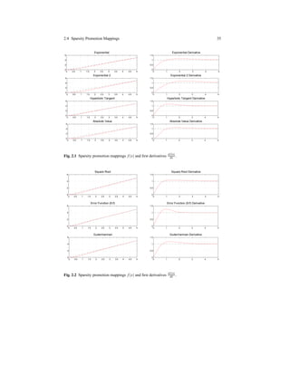
![36 2 Lipschitzian Mappings for Sparse Representation
at the origin [10]. It obeys to the shrinkage rule since |fλ (x)| ≤ |x| for all x ∈ R and
it is nondecreasing, as shown by its plotting in Figure 2.3. Just for comparison, in
figure is displayed also the soft threshold function Sτ(x) = max(|x| − τ,0)sgn(x)
which arises frequently in sparse signal processing and compressed sensing. The
latter, differently from (2.12), is discontinuous and Sτ(x) = 0 iff |x| ≤ τ.
x x
x
1−
e−
λ
|x|
x
x
m
ax(|x|−
τ
,0)sgn(x)
Fig. 2.3 The graphs of shrinking function (2.12) and the well known soft threshold function.
To deal with high dimensional data, we extend mapping (2.12) to many dimen-
sions , obtaining the one-parameter family of nonlinear mappings Fm = {Fλ : Rm →
Rm | λ ∈ R+}, where the k-th component (Fλ (x))k of Fλ
(Fλ (x))k = fλ (x), (1 ≤ k ≤ m) (2.13)
Analogously to the scalar case, the function [fλ (x1)/x1,..., fλ (xm)/xm] repre-
sents a symmetric sigmoid function in m dimensions, where larger values of λ give
sharper sigmoids, in the limit becoming a Heaviside multi-dimensional step func-
tion.
Now we come back to the problem
Φα = s
where Φ is an n×m sensing matrix of full rank, and s is the vector of observations.
The set of possible solutions AΦ,s = {x|Φx = s} is the affine space ν +NΦ, where
NΦ = {y|Φy = 0} is the null space of Φ and ν is the solution with minimum ℓ2
norm. We recall that ν = Φ†s, where Φ† = (ΦT Φ)−1ΦT is the Moore-Penrose
pseudo inverse of Φ.
Let P be the projector onto NΦ. For each x in Rm is projected in a point y ∈
AΦ,s = ν + NΦ as follow:
y = Px+ ν (2.14)
These early assumptions suggest to define a new mapping by composing the
shrinking (2.13) and the feasibility (2.14). As a consequence, we get the self-
mapping family Gλ : AΦ,s → AΦ,s, which has the form](https://image.slidesharecdn.com/f546e914-990d-4b7e-af7b-78d9394c1be8-160713201804/85/phd_unimi_R08725-52-320.jpg)


![50 2 Lipschitzian Mappings for Sparse Representation
2.5.4 The LIMAPS Algorithm
Stating the role of the parameter λ in the family of Lipschitzian-type mappings F,
we call it sparsity ratio because it determines how strong the overall increment of
the sparsity level should be within each step of the iterative process. In fact, when
applied iteratively, for small λ this kind of mappings should promote sparsity by
forcing the magnitude of all components αi to become more and more close to zero
(recall that the map is contractive within (−1/λ,1/λ)). On the other hand, for high
values of λ, the chance to reduce the magnitudes of the αi diminishes, fixing its
value over the time. Hence, for gaining sparsity, the scheduling of sparsity ratio λ
should start from small values and then increase according to the iteration step n.
This behavior is exhibited by the algorithm LIMAPS (which stands for LIPS-
CHITZIAN MAPPINGS FOR SPARSITY) introduced in [2], whose pseudo-code is
sketched in Algorithm 3.
Algorithm 3 LIMAPS
Require: - a dictionary Φ ∈ Rn×m
- its pseudo-inverse Φ†
- a signal s ∈ Rn
- a sequence {λt}t≥0
1: t ← 0
2: α ← ν
3: while [ cond ] do
4: λ ← λt <sparsity ratio update>
5: β ← fλ (α) <increase sparsity>
6: α ← β −Φ†(Φβ −s) <orthogonal projection>
7: t ← t +1 <step update>
8: end while
Ensure: a fixed-point α = Pα +ν
Remark 1 As said informally above, its ability to find desired solutions is
given by wise choices which will be adopted for the sequence {λt}t≥0, together with
choosing a good dictionary. Among many candidates respecting the constraints im-
posed by (2), one of the most promising sequence, at least on empirical grounds, is
the geometric progression whose t-th term has the form
λt = γλt−1 = θγt
for t ≥ 1,
where λ0 = θ and γ > 1 are positive and fixed constants.
Remark 2 In order to have faster computations, the projection operation P
must be split into the two matrix products of steps 5 and 6 in pseudocode LIMAPS .](https://image.slidesharecdn.com/f546e914-990d-4b7e-af7b-78d9394c1be8-160713201804/85/phd_unimi_R08725-66-320.jpg)


![2.6 Sparsity Approximation with Best k-Basis Coefficients 53
Algorithm 4 k-LIMAPS
Require: - dictionary Φ ∈ Rn×m
- signal x ∈ Rn
- least square solution ν = Φ†x
- sparsity level k
1: α ← ν
2: while [ cond ] do
3: σ ← sort (|α|)
4: λ ← 1/σk+1
5: α ← α −P α ⊙e−λ| ˆα|
6: end while
7: ˆα ← PCk
(α)
Ensure: An approximate solution ˆα ∈ Ck.
have some noise among the null coefficients, that is those with indices in the set Λc.
However, experimentally we found that such coefficients reach arbitrary close to
zero values as the number of loops increases, making the threshold step not strictly
necessary. In Fig. 2.8 we plot the α coefficients showing thus annealing-like behav-
ior which hits the not required coefficients exhibited by k-LIMAPS already at the
beginning of the first iterations.
1 15 10 15 20 25 30 1 15 10 15 20 25 30
1 15 10 15 20 25 30 1 15 10 15 20 25 30
σ15
= 0.0103 σ30
= 7.72e−04
σ15
= 0.0191 σ30
= 0.0039
Sparsity k = 10
Sparsity k = 20
Fig. 2.8 Sorted absolute values of the α coefficients. The red stencils represent the absolute values
of σt at varius times. They separate the null coefficients (black stencils) from the absolute values
of those not null (blue stencils).
The k-LIMAPS algorithm relies on the nonlinear self-mapping](https://image.slidesharecdn.com/f546e914-990d-4b7e-af7b-78d9394c1be8-160713201804/85/phd_unimi_R08725-69-320.jpg)
![54 2 Lipschitzian Mappings for Sparse Representation
α → α − P α ⊙ e−λ|α|
(2.57)
over the affine convex set (affine space) AΦ,s = {α ∈ Rm : Φα = x}, where λ > 0
is a parameter.
Starting with an initial guess α ∈ Rm and applying the mapping (2.57), the se-
quences {αt}t>0 obtained by the iterative step
αt+1 = αt − P αt ⊙ e−λt|αt|
, (2.58)
where {λt}t>0 given by (2.56). Points that at the same time minimize the problem
(LS0) and are fixed points of (2.57) are those we are looking for. To this end, after a
fixed number of iterations, k-LIMAPS uses the nonlinear orthogonal projection PCk
onto the set Ck = {β ∈ Rm : β 0 ≤ k} expressed by
PCk
(α) = arg min
β∈Ck
α − β 2
. (2.59)
Note that, due to the nonconvexity of Ck, the solution of problem (2.59) is not
unique.
2.6.1 Empirical Convergence for k-LIMAPS
To provide empirical evidence on the convergence ratio, in Fig. 2.9 we plot the
curves given by the norm
||Pαe−λ|α|
|| (2.60)
during the first simulation steps of system (2.58). They are chosen as examples
for highlighting how it behaves and how is in general the slope of the curves which
result to be decaying in all simulations. Here in particular, k-sparse random instances
s ∈ Rn and random matrix dictionaries Φ ∈ Rn×m with fixed size n = 100 and various
m = 200,...,1000. The different slopes are mainly due to the ratio m/n rather than
the values imposed to the algorithm by means of the sparsity parameter k. In fact,
the curves do not significantly change when we use values for k > k∗, where k∗ is
the optimum sparsity of the given signal s.
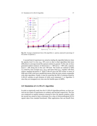
2.7 Simulation of LIMAPS Algorithm
To show the effectiveness of LIMAPS algorithm we directly compared it with some
algorithms for sparsity recovery well-known in literature, as Matching Pursuit (MP)
[77], Orthogonal Matching Pursuit (OMP) [91, 113], Stagewise Orthogonal Match-
ing Pursuit (StOMP) [45], LASSO [48], LARS [48], Smoothed L0 (SL0) [82], It-
erative Soft Thresholding [49], Accelerated iterative hard thresholding (AIHT) [17]](https://image.slidesharecdn.com/f546e914-990d-4b7e-af7b-78d9394c1be8-160713201804/85/phd_unimi_R08725-70-320.jpg)
![2.7 Simulation of LIMAPS Algorithm 55
0 10 20 30 40 50 60 70 80 90
0
0.02
0.04
0.06
0.08
0.1
0.12
0.14
0.16
m = 200
m = 400
m = 800
m= 1000
Fig. 2.9 Plotting of the norm in (2.60) with sparsity k = 10, size n = 100 and m =
200,400,800,1000.
and Improved SL0 (ISL0)[66]. In order to make the ISL0 algorithm behavior more
stable, in our implementation we used the explicit pseudo inverse calculation instead
of the conjugate gradient method, so penalizing its time performances in case of big
size instances.
In all tests, the frames Φ and the optimum coefficients α∗ are randomly generated
using the noiseless Gaussian-Bernoulli stochastic model, i.e., for all i, j ∈ [1,...,m]:
Φij ∼ N (0,n−1
) and α∗
i ∼ xi ·N (0,σ),
where xi ∼ Bern(p). In this way each coefficient α∗
i has probability p to be active
and probability 1 − p to be inactive. When the coefficient α∗
i is active, its value
is randomly drawn with a Gaussian distribution having zero mean and standard
deviation σ. Conversely, if the coefficient is not active the value is set to zero. As far
as the parameters are concerned, we fix λ0 = 10−3 and γ = 1.01 because they have
given good results in all considered instances, coming out essentially independent
from the size n × m of the frames and size m of the coefficient vectors.
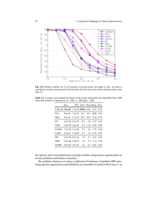
We evaluate the performances of the algorithms measuring relative error and
computation time:
1. as errors we consider the Signal-to-Noise-Ratio (SNR) and the Sum of Squares
Error (SSE) of found approximate solution α with respect the optimum α∗.
Precisely:
SNR = 20log10
α
α − α∗
, SSE = s− Φ ˆα 2
;](https://image.slidesharecdn.com/f546e914-990d-4b7e-af7b-78d9394c1be8-160713201804/85/phd_unimi_R08725-71-320.jpg)
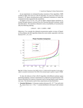
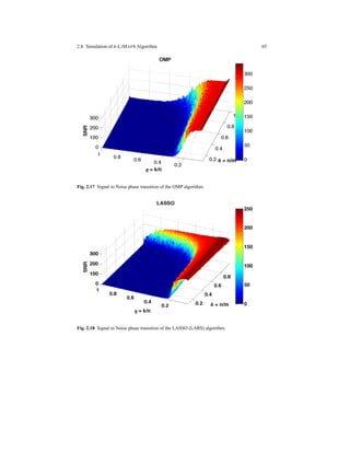
![2.8 Simulation of k-LIMAPS Algorithm 59
and an ensemble of k-sparse vectors s ∈ Rn. All matrices have been sampled from
the uniform spherical ensemble, while each vector s was a single realization of a
random variable having k nonzeros sampled from a standard iid N (0,1) distribu-
tion.
The OMP and k-LIMAPS algorithms are compared measuring their perfor-
mances on each realization according to the quantitative criterion given by the mean
square error:
MSE =
Φα − s 2
n
A diagram of the integral of the error depicts the performances of the two algo-
rithms for a wide variety of instances. The average value of such cumulative error
measure is displayed as a function of ρ = k/n and δ = n/m. Fig. 2.13 displays a grid
of δ − ρ values, with δ ranging through 50 equispaced points in the interval [.01,
.5] and ρ ranging through 100 equispaced points in [.01, 1]; here the signal length
is fixed to n = 100. Each point on the grid shows the cumulated mean square error
between the original and reconstructed, averaged over 100 independent realizations
at a given k,m.
It can be noticed that MSE of OMP increases particularly when δ tends to .5
and ρ tends to 1, while k-LIMAPS is less sensitive with respect to these saturation
values.
To show the effectiveness of our algorithm on real data, we focus on the dic-
tionary learning task for sparse representation applied to ECG signals. Instances are
taken from the Physionet bank [59], specifically in the class of normal sinus rhythm,
collecting many patient records with normal cardiac activity. We took a long ECG
registration relative to a single patient and we split the signal into segments of length
n = 128, each one corresponding to a second of the signal registration and sampled
with frequency fs = n, then we divide the blocks so obtained into two groups: train-
ing set and test set.
To perform the dictionary learning task we use KSVD[5] and MOD[50] tech-
niques working in conjunction with both the pursuit algorithm OMP and our non-
linear method k-LIMAPS as sparsity recovery algorithms. In the training phase, the
algorithms perform 50 iteration steps with a fixed sparsity level of 64 coefficients
(50% of the signal length), over a dataset collecting 512 samples randomly picked
from training set. At the end of the learning phase, the dictionaries carried out by
the learning algorithms were tested on 5000 signals picked from the test set using
the same sparse recovery algorithms (OMP or k-LIMAPS ) previously applied in
the training phase.
To evaluate the accuracy of the signal reconstruction, one of the most used perfor-
mance measure in the ECG signal processing field is the root mean square difference
or PRD, together with its normalized version PRDN (which does not depend on the
signal mean), defined respectively as:
PRD = 100 ∗
s− ˆs 2
s 2
and PRDN = 100 ∗
s− ˆs 2
s− ¯s 2
,](https://image.slidesharecdn.com/f546e914-990d-4b7e-af7b-78d9394c1be8-160713201804/85/phd_unimi_R08725-75-320.jpg)
![60 2 Lipschitzian Mappings for Sparse Representation
Fig. 2.13 Each point on the grid shows the cumulative MSE between the original s and recon-
structed Φα signals, averaged over 100 independent realizations. The grid of δ −ρ values is done
with δ ranging through 50 equispaced points in the interval [.01, 5] and ρ ranging through 100
equispaced points in [.01, 1].
where s and ˆs are the original and the reconstructed signals respectively, while ¯s is
the original signal mean.
As it can be observed in Tables 2.3 and 2.4 our sparse recovery algorithm, ap-
plied to the dictionary learning, obtains the best results on average for both training
algorithms MOD and KSVD, with standard deviations comparable to that of OMP.
The convergence error is a parameter in evaluating such a kind of algorithms.
In figure 2.14 we report all MSEs ensured by the algorithms: also in this case k-
LIMAPS outperforms OMP with both MOD and KSVD algorithms.
Qualitatively speacking, the signals recovered using dictionaries trained with
OMP suffer from a significant error in the more “flat” regions, which are mainly
localized nearby the most prominent features of a normal electrocardiogram, given
by the three graphical deflections seen on a typical ECG signal and called QRS
complex.](https://image.slidesharecdn.com/f546e914-990d-4b7e-af7b-78d9394c1be8-160713201804/85/phd_unimi_R08725-76-320.jpg)
![2.8 Simulation of k-LIMAPS Algorithm 61
Table 2.3 PRD over 5000 test signals.
PRD mean (%) PRD std. dev.
KSVD-LiMapS 15.86 5.26
MOD-LiMapS 16.16 5.05
KSVD-OMP 17.92 5.13
MOD-OMP 17.41 4.93
Table 2.4 PRDN over 5000 test signals.
PRDN mean (%) PRDN std. dev.
KSVD-LiMapS 16.17 5.26
MOD-LiMapS 15.86 5.05
KSVD-OMP 17.92 5.13
MOD-OMP 17.42 4.92
0 200 400 600 800 1000
0
1
2
3
4
5
6
7
# Iterations
Error
KSVD−LiMapS
MOD−LiMapS
KSVD−OMP
MOD−OMP
Fig. 2.14 Mean square error over the training set during each iteration of the learning process.
2.8.1 Empirical Phase Transition
Following [16], one of the main aspects of the CS systems is its ability to recover
k-sparse signals when the n ∼ k, as the problem size grows, i.e. n → ∞. Each sparse
recovery algorithm exhibits a phase transition property, such that, when no noise is
present, it exists a k∗
n such that for any ε > 0, as k∗
n, n → ∞, the algorithm successfully](https://image.slidesharecdn.com/f546e914-990d-4b7e-af7b-78d9394c1be8-160713201804/85/phd_unimi_R08725-77-320.jpg)
![62 2 Lipschitzian Mappings for Sparse Representation
recovers all k-sparse vectors, provided that k < (1 − ε)k∗
n and does not recover all
k-sparse vectors if k > (1 − ε)k∗
n.
We assume Φ is a n×m matrix with n < m, drawn from i.i.d. N (0,n−1
), the nor-
mal distribution with mean 0 and variance n−1 and let α ∈ Rm a real m dimensional
vector with k < n non zero entries.
For the problem (s,Φ) we seek the sparsest vector α such that s = Φα. When
the solution of (P1) is the same as the solution of the problem (BP0), α is called a
point of ℓ1/ℓ0 equivalence.
Following the convention used by Donoho [44], we denote ρ = k
n and δ = n
m a nor-
malized measure of problem indeterminacy and a normalized measure of the spar-
sity respectively, and we define regions (δ,ρ) ∈ [0,1]2
that describe the difficulty
of a problem instance, in which there is a high probability on the draw of Gaussian
matrix Φ that for large problem sizes (k,n,m) → ∞, all α ∈ Σk are points of ℓ1/ℓ0
equivalence.
A problem can be considered difficult to recover if the sparsity measure and the
problem indeterminacy measure are high.
The region where ℓ1/ℓ0 equivalences occur for all α ∈ Σk is given by (δ,ρ) for
ρ ≤ (1 − ε)ρS(δ) (2.61)
for any ε > 0, where the function ρS(δ) defines a curve below which there is expo-
nentially high probability on the draw of a matrix Φ with Gaussian i.i.d. entries that
every k-sparse vector is a point of ℓ1/ℓ0 equivalence .
0 1 2
0
1
n / m
k/n
Underdetermined Overderdetermined
ℓ1/ℓ0
Equivalence
Combinatorial
Search
Fig. 2.15 Donoho-Tanner [44] Phase Transition.](https://image.slidesharecdn.com/f546e914-990d-4b7e-af7b-78d9394c1be8-160713201804/85/phd_unimi_R08725-78-320.jpg)
![2.8 Simulation of k-LIMAPS Algorithm 63
Any problem instance with parameters (k,n,m), ∀ε > 0, if k
n = ρ < (1−ε)ρS(δ),
then with high probability in the draw of a matrix Φ with entries drawn i.i.d. from
N (0,n−1
) every α ∈ Σk is a point of ℓ1/ℓ0 equivalence.
Rudelson and Vershynin in [100] provided a sufficient condition under which
Gaussian matrices will recover all α ∈ Σk.
The next theorem shows the main result in terms of lower bound on the phase tran-
sition ρRV
S (δ) for Gaussian matrices.
Theorem 2.4. For any ε > 0 as (k,n,m) → ∞, there is an exponentially high prob-
ability on the draw of Φ with Gaussian i.i.d. entries that every α ∈ Σk is a point of
ℓ1/ℓ0 equivalence if ρ < (1 − ε)ρRV
S (δ), where ρRV
S (δ) is the solution of
ρ =
1
12 + 8log( 1
ρδ )β2(ρδ)
with
β(ρδ) = exp
log(1 + 2log( e
ρδ ))
4log( e
ρδ )
The curve (δ,ρRV
S (δ)) is the theoretical curve that separates the successful re-
coverability area positioned below from unrecoverable instances described by the
portion of phase space above. In Fig. 2.15, the Donoho-Tanner [44] phase transition
is illustrated. The area under the red curve represents the ℓ1/ℓ0 equivalence area.
For a given algorithm, we estimate the phase transition measuring the capability
of sparse recovery through extensive experiments. We fix the number of equations
of the undetermined system to n = 100 and we move the number of variables m and
the sparsity level k through a grid of 900 δ and 100 ρ, with δ varying from 0.01 to
1.0 and with ρ varying from 0.01 to 1.0. At each (δ,ρ) combination, we perform
100 problem instances.
Each problem instance is randomly generated using the Gaussian-Bernoulli
stochastic model, with each frame entry Φi,j ∼ N (0,n−1). Each entry belonging
to the optimal solution α∗ is modeled as
α∗
∼ xi.N (0,σ)
with xi ∼ Bern(p) distributed as a Bernoulli random variable with parameter p,
probability of coefficient’s activity. Finally the vector of known terms s of the linear
system is calculated by Φα∗ = s.
A problem instance generated as described above is thus a triplet (Φ,s,α∗) con-
sisting of a frame Φ ∈ Rn×m
and a k sparse coefficients vector α∗
.
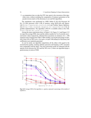
To better highlight the reconstruction performances obtained by each algorithm,
we chose to plot the phase transition plane in terms of Signal-to-Noise-Ratio (SNR),
that compares the level of the desired k sparse vector α∗ to the level of noise of the
estimated vector α.](https://image.slidesharecdn.com/f546e914-990d-4b7e-af7b-78d9394c1be8-160713201804/85/phd_unimi_R08725-79-320.jpg)


![Chapter 3
Face Recognition
Abstract In the first part of this chapter, we present a new holistic approach for
face recognition [3] that even with few training samples is robust against both
poorly defined and poorly aligned training and testing data. Working in the con-
ventional feature space yielded by the Fisher’s Linear Discriminant analysis, it uses
the sparse representation algorithm, namely k-LIMAPS introduced in chapter 2, as
general classification criterion. Thanks to its particular search strategy, it is very fast
and able to discriminate among separated classes lying in the low-dimension Fish-
erspace. In the second part of this chapter, we introduce a local-based FRS namely
k-LIMAPS LFR, proposing two possible local features: either raw sub-images or
Gabor features. Both these variants combine weak classifiers based on random local
information, creating a new robust classifier able to recognize faces in presence of
occlusions.
3.1 Introduction
In the last decades the face recognition problem has been widely studied involving
biological researchers, psychologists, and computer scientists. This interest is moti-
vated by the numerous applications it involves, such as human-computer interaction
(HCI), content-based image retrieval (CBIR), security systems and access control
systems [125]. Unfortunately there is still a big disparity between the performances
achieved by existing automatic face recognition systems (FRSs) [125, 97] and hu-
man ability in solving this task. In particular, the existing methods behave very well
under controlled conditions, but their performances drop down significantly when
dealing with uncontrolled conditions [125, 112, 97]. The term uncontrolled con-
ditions refers to several problems affecting the images, including variations in the
environmental conditions (lighting, clutter background), variations in the acquired
face (expressions, poses, occlusions), and even the quality of the acquisition (fo-
cus/blurred). All these problems have high probability to happen in real applica-
tions, thus they need to be faced to have a robust face recognition system (FRS).
71](https://image.slidesharecdn.com/f546e914-990d-4b7e-af7b-78d9394c1be8-160713201804/85/phd_unimi_R08725-87-320.jpg)
![72 3 Face Recognition
Many solutions have been proposed to face each single problem: several illumi-
nation invariant FRSs have been presented (e.g. [107, 46, 60, 83]), and also systems
dealing with variations of the expression and occlusions (e.g. [84, 7]). However,
such systems are specialized on one problem, while in real applications, it is neces-
sary a system able to deal with any possible imperfection, even added together. In
this perspective a big effort has been done: the FRSs proposed in [122, 38, 104, 95]
deal with uncontrolled images in general, achieving high performances. But again
when trying to adopt them in real applications other problems arise. The first con-
cerns the number of images per subjects required for training: many FRSs [122, 38]
behaves well only if a sufficiently representative training set is available which,
however, is not possible in many applications. On the contrary in literature we find
works where the training phase requires only one image per subject (facing the so
called Small Sample Size problem) [70, 96], but then the performances are too poor.
Another question concerns the step of face cropping: most approaches [104, 95]
present results on face images cropped using manual annotated landmarks, but this
is not indicative of the performances we would have applying the methods on au-
tomatic detected faces. In fact it has been amply demonstrated that the system per-
formances decrease drastically in presence of misalignment [18]. This problem has
been tackled in [124, 118] showing extensive results. Other factors to take into ac-
count evaluating a FRS are its scalability, namely, ”does the system perform well
even with big galleries?”, and the computational cost of the algorithm: real-time is
often required in applicative contexts.
Existing FRSs can be classified in holistic (H) and local-based (L). The holistic
approaches are suitable in case of low quality images considering they do not re-
quire to design and extract explicit features. The most popular are Eigenface [115],
Fisherface [14] and Laplacianface [64]. More recently a new approach [123] based
on the sparse representation theory [41, 25] has been proposed, proving its effec-
tiveness. This method aims at recognizing a test image as a sparse representation
of the training set, assuming that each subject can be represented as a linear com-
bination of the corresponding images in the training set. The main disadvantage of
this method, and of all the holistic approaches in general, is that it requires a very
precise (quasi-perfect) alignment of all the images both in the training and in the test
sets: even small errors affect heavily the performances [37]. Besides, they require to
have numerous images per subject for training. All these characteristics are not con-
ceivable for real world applications. The local-based methods extract local features
either on the whole face [92] or in correspondence to peculiar fiducial points [120].
By construction, such methods are more robust to variations caused by either illu-
mination or pose changes. Moreover they are more suitable to deal with face partial
occlusions [90, 79] that may occur in real world applications. Their main disad-
vantages are the computational cost and the fact that they require a certain image
resolution and quality, which cannot be guaranteed in real world applications.
In this chapter we propose both a holistic method and a local approach, high-
lighting their strengths and weaknesses.
The holistic approach follows [123], while being fast, robust and completely au-
tomatic. The crucial peculiarity consists in the adopted sparse approximation algo-](https://image.slidesharecdn.com/f546e914-990d-4b7e-af7b-78d9394c1be8-160713201804/85/phd_unimi_R08725-88-320.jpg)
![3.2 Holistic Face Recognition by k-LIMAPS Algorithm 73
rithm, solving an underdeterminend linear system using the k-LIMAPS algorithm
[2] presented in chapter 2. Such method is based on suitable Lipschitzian type map-
pings providing an easy and fast iterative scheme which leads to capture sparsity in
the face subspace spanned by the training set. With this change the method achieves
higher performances both in presence of unregistered and uncontrolled images.
The local-based approach we propose is also based on the k-LIMAPS algorithm,
while it extracts local and multiscale information (either raw sub-images or Gabor
features) in correspondence to the visible parts of faces. Such setting makes the
approach suitable to deal with partial occlusions caused by either accessories (e.g.
sunglasses, scarves or hats), or hands or hair on the faces, or even external sources
that partially occlude the camera view. The main novelty of our algorithm is that it
attempts to solve the face recognition problem with a set of weak classifiers com-
bined by the majority vote rule to create a strong FRS that classifies among multiple
linear regression models, being robust to partial occlusions and misalignments.
3.2 Holistic Face Recognition by k-LIMAPS Algorithm
In this section we propose a completely automatic and fast FRS based on the sparse
representation (SR) method. Both the training and the test sets are preprocessed
with the off-the-shelf face detector presented in [116] plus the eyes and mouth lo-
cator presented in [19]. The obtained face sub-images are projected in the Fisher
space and then sparsity is accomplished applying the recently proposed algorithm
k-LIMAPS [2]. Such method is based on suitable Lipschitzian type mappings pro-
viding an easy and fast iterative scheme which leads to capture sparsity in the face
subspace spanned by the training set.
We tested out method on the Yale, Yale B Extended [56], ORL [88], BANCA [11]
and FRGC version 2.0 database [93], and compared it with the SRC method. These
experiments prove that, despite the system is completely automatic, it is robust with
respect to misalignments and variations in expression or illumination.
3.2.1 Eigenfaces and Fisherfaces
Holistic Face Recognition algorithms deal with face images trying to extract global
features describing the face in its wholeness. In this section we outline two fun-
damental techniques used to extract interesting features useful for solving the face
recognition problem. These techniques are low sensitive to large variations in light-
ing intensity, direction and number of light sources and to different facial expres-
sions.
The first is the principal component analysis (PCA) that extracts a set of features
called Eigenfaces which maximize the total scatter over the whole training set. The
second method exploits the information given by the labels of the training set to](https://image.slidesharecdn.com/f546e914-990d-4b7e-af7b-78d9394c1be8-160713201804/85/phd_unimi_R08725-89-320.jpg)
![74 3 Face Recognition
extract features called Fisherfaces which are the most discriminative as possible
among the different classes.
3.2.1.1 Eigenfaces
The Eigenface method [114, 69], is based on the principal component analysis
(PCA) also called Karhunen–Lo´eve transformation for dimensionality reduction .
It applies a linear projection from the image space to a lower dimensional feature
space so that the chosen directions maximize the total scatter across all classes, i.e.
across all images of all faces. Choosing the projection which maximizes total scatter,
the principal component analysis retains unwanted variations such as for example
facial expressions and illuminations.
Let {x1,...,xN} with xi ∈ Rn be a set of N images taking values in an n-
dimensional image space, and assume that each image xi belongs to one of the C
classes {1,...,C}. Let us consider a linear transformation mapping the original n-
dimensional image space into an l-dimensional feature space , with l < n. The new
feature vectors yi ∈ Rl are defined by:
yi = WT
xi with i = 1,...,N (3.1)
where W ∈ Rn×l is an orthonormal column matrix.
Let ST the total scatter matrix defined as
ST =
N
∑
i=1
(xi − µ)(xi − µ)T
where µ ∈ Rn is the mean image of all samples, then after applying the linear trans-
formation WT , the scatter of the transformed feature vector {y1,...,yN} is WT STW.
Principal component analysis choose the projection Wopt such that the determinant
of the total scatter matrix of the projected samples is maximized
Wopt = argmax WT
STW
with Wopt = [w1,...,wl] is the set of n-dimensional eigenvectors of ST corre-
sponding to the l largest eigenvalues . Considering these eigenvectors have the same
dimension of the original images, they are also called Eigenfaces.
If the principal component analysis is presented with images of faces under
varying illumination , the projection matrix Wopt will contain principal components
which retain, in the projected feature space, the variation due to lighting. For this
reason, the points in the projected space will not be well clustered according to the
subject identity.
The eigenvectors that catch the variance of lighting are the first eigenvectors,
thus, discarding them permits a reduction of the variation due to lighting, and con-
sequently a better clustering of the projected samples.](https://image.slidesharecdn.com/f546e914-990d-4b7e-af7b-78d9394c1be8-160713201804/85/phd_unimi_R08725-90-320.jpg)
![3.2 Holistic Face Recognition by k-LIMAPS Algorithm 75
Fig. 3.1 Examples of Eigenfaces of some subjects of the YaleB database.
3.2.1.2 Fisherfaces
The principal component analysis projections are optimal for reconstruction from
a low dimensional basis but they may not be optimal from a discrimination stand-
point.
Since the learning set is labeled, it makes sense to use this information to build a
more reliable method for reducing the dimensionality of the feature space .
Fisher Linear Discriminant analysis (FLD) [54, 14] is a class specific method,
in the sense that it tries to reshape the scatter in order to make it more reliable for
classification. This method selects the projection matrix W of (3.1) such that the
ratio of the between class scatter and the within class scatter is maximized. We
define the between class scatter matrix as:
SB =
C
∑
i=1
Ni(µi − µ)(µi − µ)T
and let the within class scatter matrix be
SW =
C
∑
i=1
∑
xj∈Xi
(xj − µi)(xj − µi)T
where µi is the mean image of the class Xi and Ni the number of samples in the
class Xi. If SW is non singular, the optimal projection Wopt is chosen as the matrix
with orthonormal columns which maximizes the ratio between the determinants of
the between and the within class scatter matrix of the projected samples respectively
Wopt = argmax
W
WT SBW
|WT SWW|
(3.2)
The matrix Wopt = [w1,...,wl] is the matrix that contains the generalized eigen-
vectors of SB and SW corresponding to the l generalized eigenvalues](https://image.slidesharecdn.com/f546e914-990d-4b7e-af7b-78d9394c1be8-160713201804/85/phd_unimi_R08725-91-320.jpg)
![76 3 Face Recognition
SBwi = λiSW wi with i = 1,...,l
Fig. 3.2 Examples of Fisherfaces of some subjects of the YaleB database.
The maximum number of nonzero generalized eigenvalues is C − 1, so an upper
bound on l is C − 1, where C is the number of classes.
In the face recognition problem, a possible difficulty that can be appear is that the
within class scatter matrix SW ∈ Rn×n can be singular. This stems from the fact that
the rank of the matrix SW is at most N −C, and in general the number of images N in
the learning set is much smaller then the number n of pixels in each image, making
possible to choose the matrix W such that the within class scatter of the projected
samples can be made exactly zero.
To avoid this problem in [14] it was proposed an alternative to the criterion (3.2)
called Fisherfaces , that projects the image set to a lower dimensional space such
that the within class scatter matrix SW is nonsingular . This can be achieved by using
the principal component analysis to reduce the dimensions of the feature space to
N −C and then applying the standard Fisher linear discriminant (3.2) to reduce the
dimension to C − 1. The projection matrix Wopt can be rewritten as
WT
opt = WT
fldWT
pca (3.3)
where
Wpca = argmax
W
WT
STW
Wfld = argmax
W
WTWT
pcaSBWpcaW
WTWT
pcaSWWpcaW
where Wpca is the projection matrix of the principal component analysis and Wfld
is the projection matrix of the Fisher linear discriminant.](https://image.slidesharecdn.com/f546e914-990d-4b7e-af7b-78d9394c1be8-160713201804/85/phd_unimi_R08725-92-320.jpg)
![3.2 Holistic Face Recognition by k-LIMAPS Algorithm 77
3.2.2 Classification Based on Linear Sparse Representation
The classification process aiming at identifying a subject within a fixed group of
individuals can be successfully carried out using techniques based on sparse repre-
sentation [123].
This process can be recasted into the problem of finding the sparsest represen-
tation of a test image, usually represented by a vector in a suitable feature space
x ∈ X ⊆ Rn, into a frame (called dictionary in this context) Φ = [φ1,...,φm] as-
sumed to be a wide collection (m > n) of vectors (or atoms ) in X , each one coding
a subject belonging to a fixed training set. In this setting, a sparse representation for
x means to linearly combine the fewest possible training images, i.e., the smallest
number of atoms such that x = ∑i αiφi, or equivalently in matricial form
Φα = x. (3.4)
Ideally, under condition of underdetermination of the system (3.4) the sparsest
solution can be found as a unique solution of the NP-hard optimization problem
BP0
In order to make effective the general techniques based on sparsity promotion
two main issues must be taken into account:
1. projection – it helps both in extracting holistic features to discriminate among
subjects and in projecting high-dimensional face images to low-dimensional
feature spaces, so making computations faster.
2. approximation – the recovery by the exact superposition of few atoms is some-
times unlikely for holistic feature spaces, therefore it is better for the sparse rep-
resentation to focus on constructing the best approximation of an image with a
linear combination of k, or fewer, atoms from the dictionary, as stated by the
sparse approximation problem:
min
α∈Rm
Φα − x subject to α 0 ≤ k, (LS0)
where · represents the standard Euclidean norm.
Following [123], the previous defined sparsity framework can be used to deter-
mine, given c distinct classes or subjects, at which one a given test image belongs.
To this end data are arranged such that the training samples from the i-th class are
represented as column vectors of the matrix Ai = [x1,...,xni ] ∈ Rn×ni. The training
set collecting all subjects is then obtained by stacking all matrices Ai into matrix
A = [A1,...,Ac].
As a usual practice, a dimensional reduction is carried out by linearly project-
ing high-dimensional face images to low-dimensional feature spaces by means of a
suitable matrix W. Thus the dictionary Φ for the sparse recovery is determined as
Φ =W A. Successively, in the classification stage, given a test image x, the projected
sample y = W x is used to find a sparse vector α such that Φα ≈ y, i.e., to solve one
out the many sparsity problems as, for instance, the problem referred by (LS0).](https://image.slidesharecdn.com/f546e914-990d-4b7e-af7b-78d9394c1be8-160713201804/85/phd_unimi_R08725-93-320.jpg)
![78 3 Face Recognition
In the purpose of solving the membership i of the test image x, one looks for
the linear span of the training samples associated to the subject i that better ap-
proximates the feature vector y. In other words, by denoting with ˆαi the coefficient
vector whose only nonzero entries are the ones in α associated to class i (zeroing
all others entries), the identity of y is found minimizing the residual with the linear
combination Φ ˆαi, i.e., by applying the discrepancy rule:
identity(y) = argmini∈[1,..,c] y− Φ ˆαi . (3.5)
3.2.3 Classification by k-LIMAPS
The holistic FRS we propose here, namely k-LIMAPS HFR, follows the setting
of the general framework introduced in the previous section, while adopting the
k-LIMAPS algorithm to solve the sparsity promotion.
The entire process for face recognition using k-LIMAPS is summarized in the
flow diagram of Figure 3.3 and consists in the following steps.
Fig. 3.3 The k-LIMAPS FR system.
1. Projection – which embed training and test n-dimensional images in the LDA
space ((c − 1)-dimensional vectors) in order to extracts holistic facial features
using the matrix WLDA as projector.
2. Sparsity – which finds a sparse representation of a test image x by building the
dictionary Φ =WLDA A ∈ R(c−1)×n (with c−1 < n) and applying k-LIMAPS to](https://image.slidesharecdn.com/f546e914-990d-4b7e-af7b-78d9394c1be8-160713201804/85/phd_unimi_R08725-94-320.jpg)
![3.2 Holistic Face Recognition by k-LIMAPS Algorithm 79
the projected test image y =WLDA x using dictionary Φ, an initial guess α0 = Py,
and the sparsity parameter s.
Classify – which finds the identity of x by applying rule (3.5).
3.2.4 Databases
As claimed before, our goal is to define a FRS that works independently of the ac-
quisition conditions. In order to verify this independence, we test our FRS on several
databases that differ significantly one from the others with respect to several aspects:
the illumination conditions, the photo sharpness, the face pose and expression, the
context, and the subject cardinality. In particular in table (3.1) we report the results
obtained on the following databases:
1. Yale db: contains 165 grayscale images of 15 individuals with homogeneous
background. There are 11 images per subject, where the expression (neutral,
happy, sad, sleepy, and wink) and the illumination conditions (central/right/left-
light) are varied. The subjects are also acquired both with or without glasses.
2. YaleB + Extended YaleB db [56]: contains 21888 grayscale images of 38 in-
dividuals acquired in 9 poses and 64 different illuminations, all with homoge-
neous background. For our experiments we considered the images with frontal
faces under any illumination conditions (2432 images).
3. ORL db [88]: contains 400 grayscale images of 40 distinct subjects in frontal
position and with homogeneous background.The images were taken at different
times, varying the lighting, facial expressions (open / closed eyes, smiling / not
smiling) and facial details (glasses / no glasses).
4. BANCA db [11]: it is a large, realistic and challenging multi-modal database.
For our experiments we refer to the sections Controlled and Adverse. Con-
trolled: it consists of 2080 images of of 52 people placed in front of the camera
and looking down as if reading. The images were acquired in 4 different ses-
sions. The images have homogeneous background while the illumination condi-
tions vary from daylight to underexposed. Adverse: like the Controlled section
it consists of 2080 images. The main difference is that the background is non-
uniform and the image quality and illumination are poorer.
5. FRGC version 2.0 db [93]: this dataset reports images of 466 people acquired
in several sessions (from 1 to 22, varying from person to person), over two pe-
riods (Fall 2003 and Spring 2004). A session consists of six images: four con-
trolled and two uncontrolled, both acquired with either neutral or smiling face
expression. Controlled images are acquired in frontal pose, with homogeneous
illumination, while the uncontrolled ones represent smaller faces, often blurred
and acquired in several illumination conditions. For our experiments we con-
sidered only the subjects with at least three sessions per period. This brought us
to 384 subjects, in the case of the uncontrolled section, and 394 subjects for the
controlled one.](https://image.slidesharecdn.com/f546e914-990d-4b7e-af7b-78d9394c1be8-160713201804/85/phd_unimi_R08725-95-320.jpg)
![80 3 Face Recognition
Table 3.1 Database description. From the left to the right the columns are the database name,
number of subjects, number of images, background, illumination, expression, timing and the image
quality.
Database N. sbj N. Imgs. Back. Illum. Expr. Timing Qual.
Yale 15 165 hom. varies varies n good
ORL 40 400 hom. varies varies y good
BANCA Controlled 52 2080 hom. good reading y good
BANCA Adverse 52 2080 clutter poor reading y bad
Extended Yale B (frontal) 38 2432 hom. varies neutral n good
FRGC v.2 Controlled 394 5726 hom. good varies y good
FRGC v.2 Uncontrolled 384 5248 clutter poor varies y bad
3.2.5 Experimental results
In this section we present the experimental results obtained running our system
on several public databases.
All the experiments have been carried out on images automatically localized
with the face detector proposed in [117] followed by the eyes and mouth locator
presented in [19]. No human intervention is required. The misalignment we deal
with is exemplified in Fig. 3.4.
Fig. 3.4 Examples of automatic cropping on uncontrolled images (first line from the FRGC v.2
db; second line from the BANCA Adverse db).
The number of images in the training set has been deliberately kept low (k vary-
ing between 3 and 5) in order to emulate real world settings. The results we
report have been obtained mediating over 100 trials; at each iteration, k images
are randomly selected for training and the remaining are used to construct the
test set. Comparisons have been carried out with the state-of-the-art SRC [123],
with a feature space dimension equal to 100, which is a good compromise be-
tween the performances and the computational costs.
We first set up several experiments referring to a subset of the FRGC 2.0 dataset.
The choice of this database is due to its high subject cardinality and to its rich-](https://image.slidesharecdn.com/f546e914-990d-4b7e-af7b-78d9394c1be8-160713201804/85/phd_unimi_R08725-96-320.jpg)

![82 3 Face Recognition
ORL and the FRGC v.2 Controlled and Uncontrolled. With this experiment
we wanted to demonstrate the robustness of our method independently of the
database in analysis.
Table 3.4 The face recognition rate (%) on some databases.
Database k = 3 k = 4 k = 5
k-LIMAPS HFR SRC k-LIMAPS HFR SRC k-LIMAPS HFR SRC
Yale 95.7 (26) 36.7 97.4 (46) 39.9 98.0 (44) 41.0
ORL 89.6 (52) 65.5 93.0 (66) 83.0 95.3 (54) 89.4
BANCA Co. 90.8 (148) 81.1 94.3 (154) 89.9 96.5 (190) 93.8
BANCA Ad. 86.3 (148) 77.4 90.7 (154) 87.5 93.9 (198) 91.9
Ext. Yale B 89.3 (109) 45.7 94.2 (114) 69.9 96.3 (146) 79.7
FRGC v.2 Co. 90.1 (565) 87.8 94.0 (625) 92.4 96.0 (685) 94.4
FRGC v.2 Un. 72.5 (530) 65.6 79.7 (530) 72.1 84.6 (634) 75.1
The experiments have been carried out keeping low the number of images per
subjects in the training set and repeating 100 times each single setting. In table
3.4 we report the average results; regarding the standard deviations, we remark
they are always very low (varying between 0.013 and 0.019), indicating a good
stability of the system. Results are presented for each database, reporting for
each k: the best results obtained varying the number of features n (in brackets
we indicate the corresponding value of n) and the results obtained on the same
data running the SRC algorithm.
In the following we highlight some aspects crucial for the applicability of the
system in real applications: the robustness to possible misalignment produced
by the localization step (sec. 3.2.5.1); the low criticality of the parameter set-
ting (sec. 3.2.5.2); the robustness in a wide range of acquisition conditions
(sec. 3.2.4); the low computational cost in testing phase (sec. 3.2.5.3).
3.2.5.1 Face localization
In all the experiments the images have been cropped automatically: we applied
the face detector proposed in [116], followed by the eyes and mouth locator
(EML) presented in [19]. The faces missed by the Viola-Jones face detector are
not considered for the subsequent steps, while the misalignments caused by the
EML is managed by the FRS.
In order to give a quantitative estimate of the misalignment error, we computed
the relative error measure introduced by Jesorsky [67] defined as
deye =
max(||Cl − ˜Cl||,||Cr − ˜Cr||)
||Cl −Cr||](https://image.slidesharecdn.com/f546e914-990d-4b7e-af7b-78d9394c1be8-160713201804/85/phd_unimi_R08725-98-320.jpg)

![84 3 Face Recognition
on the other hand, it is computational very expensive preventing by itself the
applicability in real applications.
The k-LIMAPS HFR is very fast being based on an iterative search strategy,
that in the case of face recognition arrives to convergence after few iterations
(namely 5-10).
In particular, the MATLAB implementation of our algorithm runs each image
in 0.01 seconds when referring to the most populous dictionary (FRGC con-
trolled), resulting in a real-time solution for the FR problem.
3.3 Face Recognition with Occlusions by k-LIMAPS
Occlusions and variation of expressions are the most common difficulties in
applications involving automatic FRSs. Sources of occlusions can be apparel
like sunglasses, eyeglasses, scarves and hats as well as hands or hair covering
part of a face or even other objects placed between the camera and the face.
Other kind of occlusions can be considered extreme variation of illumination
like dark shadows or excessive lighting.
Robustness to occlusions is essential for real world FRSs. If faces are partially
occluded, holistic methods based on Eigenfaces of Fisherfaces [14] cannot be
applied, since all the features extracted from the training set would be corrupted.
In this work we propose a local-based FRS namely k-LIMAPS LFR, com-
bining a set of weak local classifiers obtaining a strong and robust classifier,
suitable to solve the face recognition problem under occlusions. This algorithm
exploits two possible local features: the first, described in 3.3.2, called Multi-
scale Random Tessellations (MRT), consist of natural patches extracted from
face images; the second, are Gabor features (Gf) that well describe contours
and local variations in spatial domain.
The k-LIMAPS LFR system consists of two phases: the dictionary construction
and the test phase. Regarding the first one, we proceed selecting k unoccluded
images per subject and extracting from each of them a high number Z, of local
features (the same pool of features for all the images). Z dictionaries are then
constructed, one for each feature z, linearizing the corresponding information
extracted from each training images and placing them side by side in the matrix
Φz.
The testing phase is articulated in the following steps. At first the test image
is classified according to the possible occlusion (unoccluded / glasses / scarf)
performed through the use of the EML locator. In the case the EML locator cor-
rectly localize eyes, the subject must be checked by the scarf detector described
in [80] in order to determine the scarf possible presence. Otherwise, if the EML
fails to locate eyes, the face are classified as occluded by sunglasses. On the
basis of this information, we inhibit the occluded regions referring to off-line
defined masks. In particular two binary masks, one corresponding to sunglasses
and the other to scarves. The masks are mathematically described as M(x,y):](https://image.slidesharecdn.com/f546e914-990d-4b7e-af7b-78d9394c1be8-160713201804/85/phd_unimi_R08725-100-320.jpg)
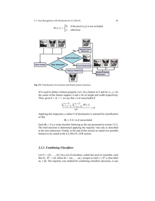
![86 3 Face Recognition
of many methods that assign to x the class label ωj that is supported by the
majority of the classifiers Di.
In general given the votes of L classifiers D1,...,DL, we define a majority vote
classifier as follows
C(x) = argmax
i
L
∑
j=1
wjI(Dj(x) = i) (3.6)
where w1,...,wL are weights such that ∑j wj = 1, and I(.) is an indicator func-
tion. If weights are wj = 1
L , (3.6) can be rewritten as
C(x) = mode{D1(x),...,DL(x)} (3.7)
where mode(.) is the value that appears most often in the set of classifiers.
Finding independent classifiers is one aim of classifier fusion methods for the
following reason. Let L be odd, Ω = {ω1,ω2}, and all classifiers have the same
classification accuracy p ∈ [0,1]. The majority vote method with independent
classifiers decisions gives an overall correct classification accuracy calculated
by the binomial formula
pma j =
⌊L/2⌋
∑
i=0
L
i
pL−i
(1 − p)i
where ⌊x⌋ denotes the largest integer less than or equal to x. The majority vote
method with independent classifiers is guaranteed to give a higher accuracy than
individual classifiers when p > 0.5 [72, 71].
3.3.2 Local Features
The first pool of features we are interested in investigating consists of patches
extracted varying randomly the position, the height and the width. These raw
data capture local details, varying the scale and thus the retailed details.
In figure 3.6 we can see examples of random patches maintained in presence
of different kind of occlusions. We observe that both the screaming and neutral
expression images are unoccluded, thus their occlusion masks are set to 0 for
all pixels.
The second pool of features we investigate is obtained applying a bank of Gabor
filters in correspondence to a certain number of points randomly extracted from
the non occluded face portion.
A Gabor filter is a linear band pass filter, widely used for edge detection, ob-
tained by modulating an harmonic sinusoidal function with a Gaussian function.
The filter has a real and an imaginary component representing orthogonal di-
rections.](https://image.slidesharecdn.com/f546e914-990d-4b7e-af7b-78d9394c1be8-160713201804/85/phd_unimi_R08725-102-320.jpg)
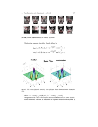
![88 3 Face Recognition
specifies the ellipticity of the support of the Gabor function and φ is the phase
offset.
The real and the imaginary components of the Gabor filter may be used individ-
ually or combined to form a complex number as defined below:
g(x,y;λ,θ,φ,σ,γ) = e
− x′2
+y′2
γ2
2σ2 ei(2π x′
λ +φ)
The response of a Gabor filter to an image is obtained by a 2D convolution
operation. Let I(x,y) denotes the image and let G(x,y;λ,θ,φ,σ,γ) be the re-
sponse of a Gabor filter g(x,y;λ,θ,φ,σ,γ) at point (x,y) on the image plane.
The response G(.) of the Gabor filter is obtained as
G(x,y;λ,θ,φ,σ,γ) = I(u,v)∗ g(x,y;λ,θ,φ,σ,γ)
=
+∞
−∞
I(u,v)g(x− u,y− v;λ,θ,φ,σ,γ)dudv
In figure 3.8 we show the amplitude of response of Gabor filters with different
orientations and scales applied to a face image.
Wiskott at al. in [121] suggest a set of Gabor filters with 5 spatial frequencies
and 8 distinct orientations to create an efficient filter bank.
Parameters are resumed in table 3.5
Table 3.5 Parameters of Gabor filters.
Parameter Symbol Values
Orientation θ {0, π
8 , 2π
8 , 3π
8 , 4π
8 , 5π
8 , 6π
8 , 7π
8 }
Wavelength λ {4,4
√
2],8,8
√
2,16}
Phase φ {0, π
2 }
Gaussian Radius σ {4,4
√
2],8,8
√
2,16}
Aspect Radius γ 1
Gabor filters are among the most popular tools for facial feature extraction.
Their use in automatic face recognition system is motivated by two major fac-
tors: their computational properties and their biological relevance.
When exploited for feature extraction, a filter bank with several filters is usually
created and used to extract multiorientational and multi-scale features from the
given face image.
By convolving face images with the Gabor kernels of the filter bank previously
defined, we would have a total of 40 Gabor filter response images. These im-
ages could be used as features, but their high dimensionality would make this
approach impractical.
To reduce the feature space, our approach consists in generating random points
spatially located in non occluded area of the image, and in calculating local
features through the application of the Gabor filter bank.](https://image.slidesharecdn.com/f546e914-990d-4b7e-af7b-78d9394c1be8-160713201804/85/phd_unimi_R08725-104-320.jpg)
![3.3 Face Recognition with Occlusions by k-LIMAPS 89
5 10 15 20 25 30 35 40 45 50
10
20
30
40
50
60
5 10 15 20 25 30 35 40 45 50
10
20
30
40
50
60
5 10 15 20 25 30 35 40 45 50
10
20
30
40
50
60
5 10 15 20 25 30 35 40 45 50
10
20
30
40
50
60
5 10 15 20 25 30 35 40 45 50
10
20
30
40
50
60
5 10 15 20 25 30 35 40 45 50
10
20
30
40
50
60
Fig. 3.8 Example of features extracted convolving a subject with Gabor filters with different ori-
entations and scales.
3.3.3 Occlusion and Expression Database
Our goal is to test the k-LIMAPS LFRS system in case of partial occlusions
or expression variations. To this end we adopted the AR [78] database that con-
tains images of faces acquired with different occlusions and with different ex-
pressions.
This face database was created by Aleix Martinez and Robert Benavente in
the Computer Vision Center (CVC) at the U.A.B. It contains over 4,000 color
images corresponding to 126 people’s faces (70 men and 56 women). Images
show frontal view faces with different facial expressions, illumination condi-
tions, and occlusions (sun-glasses and scarves). The pictures were taken at the
CVC under strictly controlled conditions. No restriction on clothing, make-up,
hair style, etc. were imposed to participants. Each person participated in two
sessions, separated by two weeks (14 days) time.
The same pictures were taken in both sessions.
All images are stored in raw file format of the form G-xx-yy.raw. The letter ’G’
represents the gender of the subject and can assume the value ”M” for males
and ”F” for females, ’xx’ is a unique person identifier (from ”00” to ”70” for
males and from ”00” to ”56” for females) and ’yy’ specifies the features of each
image; its meanings are described in the following table:
1 Neutral expression
2 Smile
3 Anger
4 Scream
5 left light on
6 right light on
7 all side lights on
8 wearing sun glasses
9 wearing sun glasses and left light on
10 wearing sun glasses and right light on
11 wearing scarf
12 wearing scarf and left light on
13 wearing scarf and right light on
14 to 26 second session (same conditions as 1 to 13)](https://image.slidesharecdn.com/f546e914-990d-4b7e-af7b-78d9394c1be8-160713201804/85/phd_unimi_R08725-105-320.jpg)
![90 3 Face Recognition
3.3.4 Experimental results
In this section we present the experimental results obtained on the AR database run-
ning our local-FRS using both Multiscale Random Tessellation and Gabor features
.
Table 3.6 Face recognition rate (%) for AR registered with 100 subjects, 100 trials.
k-LIMAPS LFR k-LIMAPS LFR SRC PFI
Type Train Test MRT Gf
200 pieces 300 points
1 Glasses [1 : 4,14 : 17] [8,21] 98.15 94.50 97.50 97.50
2 Scarf [1 : 4,14 : 17] [11,24] 98.27 97.30 93.00 93.50
3 Glasses [1,5 : 7,14,18 : 20] [8 : 10,21 : 23] 95.01 95.00 96.00 97.70
4 Scarf [1,5 : 7,14,18 : 20] [11 : 13,24 : 26] 96.45 97.17 91.50 82.50
5 Glasses [1,2,5 : 7] [8 : 10,21 : 23] 87.80 91.30 79.30 84.50
6 Scarf [1,2,5 : 7] [11 : 13,24 : 26] 92.05 95.53 82.30 73.20
7 Neutral [1,2,5 : 7] [14,15,18 : 20] 98.94 99.76 96.20 98.80
8 Expression [1 : 4,7] [15 : 17] 95.77 96.47 91.00 97.00
In all the experiments the images are automatically located with the face detector
proposed in [117] and automatically registered by the eyes and mouth locator (EML)
presented in [19]. In case of sunglasses, the EML reports the eyes absence, thus
we refer to the face localized by the face detector. In case of scarves, the eyes are
generally correctly localized, allowing a partial registration.
The results we report have been obtained mediating over 100 experiments, vary-
ing randomly the patches for the Multiscale Random Tessellation (MRT) and the
point locations for the Gabor features (Gf).
We setup two sessions of experiments. In the first we adopt 8 images per subject
for the training set (k = 8), according to the experiments reported in literature [123].
In the second we reduce k to 5 in order to test the system behavior in more realistic
conditions. In all cases the training images are non occluded. Comparisons have
been carried out with the state-of-the-art SRC [123] and with the algorithm proposed
in [103, 105] that use a large features sets extracted locally in each image.
In the first session, the training sets are constructed as proposed in [123]. In
particular the authors propose two scenarios: in the first (adopted for the experiments
1 and 2 in the table (3.6)) the training sets represents each subject under different
expressions, while the illumination condition is constant. In the second (adopted for
the experiments 3 and 4 in the table (3.6)), the expression is always neutral while
the illumination conditions vary over the training images. In the second session all
illumination and neutral and smiling expressions are used for training. Only in the](https://image.slidesharecdn.com/f546e914-990d-4b7e-af7b-78d9394c1be8-160713201804/85/phd_unimi_R08725-106-320.jpg)
![3.3 Face Recognition with Occlusions by k-LIMAPS 91
case of test over the expressions, we enrich the training with all the expressions,
reducing the illumination variability.
Experiments are run both on manually registered images and on automatic regis-
tered images. Results are respectively summarized in in table (3.6) and in table (3.7).
We observe that in all the experiments we obtained a very low standard deviation,
varying between 0.022 and 0.037 indicating good stability results.
Table 3.7 Face recognition rate (%) for AR unregistered with 72 subjects, 100 trials.
k-LIMAPS k-LIMAPS SRC PFI
Type Train Test MRT GC
200 pieces 300 points
1 Glasses [1 : 4,14 : 17] [8,21] 84.40 82.74 52.56 83.80
2 Scarf [1 : 4,14 : 17] [11,24] 95.51 96.50 88.46 70.90
3 Glasses [1,5 : 7,14,18 : 20] [8 : 10,21 : 23] 78.21 81.60 56.55 74.50
4 Scarf [1,5 : 7,14,18 : 20] [11 : 13,24 : 26] 92.86 95.95 84.33 71.40
5 Glasses [1,2,5 : 7] [8 : 10,21 : 23] 65.60 66.84 44.02 62.80
6 Scarf [1,2,5 : 7] [11 : 13,24 : 26] 87.18 91.42 75.50 64.20
7 Neutral [1,2,5 : 7] [14,15,18 : 20] 91.64 94.02 83.59 92.50
8 Expression [1 : 4,7] [15 : 17] 80.80 85.76 74.64 91.20
As we can see in table 3.6, our local-FRS using 300 Gabor features results the
best classifier in almost all cases, except for the first experiment that use training
images with controlled frontal illumination but with variations in expressions. In
this case the best results are obtained adopting the MRT features. This behavior of
the Gabor features could be explained by the fact that the Gabor filter bank is very
sensitive to edges caused by expression variations, corrupting the training informa-
tion.
In the second most realistic scenario, where the images are automatically reg-
istered, the worst performances are obtained in the case of glasses occlusion. This
result confirms the difficulty already shown in table 3.6 of recognizing a person
viewing only the lower half of the face. Here the performance drop down even more
because of the higher misalignment: in case of occlusion only the face detector is
adopted to locate the face.
As general consideration we can remark that the local-based FRS does not re-
quire specific tuning, except the number of features to generate randomly. Obvi-
ously, a small feature cardinality Z would compromise the system performances, but
at a certain level we observed that further increasing of Z would be useless for the
performance improvement, while augmenting significantly the computational costs.
Experimentally we set Z = 300 as a trade-off between performances and compu-
tational costs. In any case, considering the weak classifiers are independent, it may](https://image.slidesharecdn.com/f546e914-990d-4b7e-af7b-78d9394c1be8-160713201804/85/phd_unimi_R08725-107-320.jpg)


![94 4 ECG Signal Compression
The lossless algorithms such as the Run-Length Encoding [74], Huffman [65]
and Lempel-Ziv-Welch [119] do not show reconstruction error while the compres-
sion ratio (CR) is generally small, conversely the lossy algorithms like Foveation-
SPIHT[32] and DCeq-MMP [51] pay a quantization error to obtain higher compres-
sion level.
The most classical compression algorithms apply some data transformations to
extract the most informative characteristics exploiting the redundancy of data. The
most informative coefficients are then encoded using different lossless compression
algorithms.
Within this group many methods based on the Discrete Wavelet Transform
(DWT) [4], like the Set Partitioning in Hierarchical Tree (SPIHT) algorithm [73]
show good results in ECG signal coding.
In recent years, compressive sensing and sparse recovery theory has generated
significant interest in the signal processing community because of its potential to
enable signal reconstruction from significantly fewer data samples than suggested
by conventional sampling theory. Compared to conventional ECG compression al-
gorithms, sparse recovery has some important advantages:
(a) It transfers the computational burden from the encoder to the decoder, and thus
offers simpler hardware implementations for the encoder.
(b) The location of the largest coefficients in the wavelet domain does not need to
be encoded.
Based on the fact that electrocardiogram (ECG) signals can be approximated by a
linear combination of a few coefficients taken from a Wavelet basis, in [94] com-
pressed sensing-based approach for ECG signal compression. For solving ECG de-
noising and compression problem, in [58] was proposed an algorithm based on a
sparse separable 2-dimensional transform for both complete and overcomplete dic-
tionaries.
In this chapter we propose a new compression algorithm that seeks, for each
block of a signal, the sparsest solution of an underdetermined linear system, in a
frame generated on the basis of the first second of the signal itself.
Conversely to the algorithms in the literature, we do not compress the signal
using random projection in a lower space, but we use the sparsest representation of
the signal in a natural basis.
4.2 The Electrocardiogram
A great variety of electrical signals are produced by the human body due to the
chemical activities both in the nerves and in the muscles. Among the others, the
heart leads to a characteristic pattern of voltage variations.
The registration and analysis of these bioelectrical activities are very important
processes in fields such as the clinical research.](https://image.slidesharecdn.com/f546e914-990d-4b7e-af7b-78d9394c1be8-160713201804/85/phd_unimi_R08725-110-320.jpg)
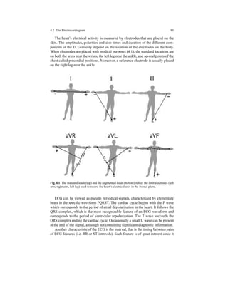
![96 4 ECG Signal Compression
Fig. 4.2 Wave definitions of the cardiac cycle. In figure are noted the P wave, the QRS complex,
the T wave and the R-R interval.
provides a measure of the state of the heart and can indicate the presence of certain
cardiological conditions [34] or diseases.
4.3 ECG Preprocessing
The aim of the preprocessing phase is to improve the quality of the electrocardio-
gram signals. The kinds of noise that can disturb the ECG signal are both low fre-
quency baseline wander (BW) and high frequency (50-60 Hz) noise. The first is
caused by the respiratory activity while the latter by either electrical power line,
poor electrode contacts, body movements or muscular activities.
In the next subsections we describe the preprocessing phase used to suppress
noise in our experiments.
4.3.1 Baseline Wander
Some considerations should be taken into account in designing a linear time invari-
ant highpass filter aimed at removing the baseline wander:
• The cut-off frequency should be chosen so that the clinical information in the
ECG signal remains undistorted while the baseline wander is removed. Indeed, if
we chose a too high cut-off frequency, the filtered signal would contain unwanted
artifacts with oscillatory component highly correlated to the beat rate. To this end
a reasonable cut-off can be fixed at 0.5 Hz: if the patient is retired, the frequency
content of the baseline wander is usually below 0.5 Hz and the lowest frequency
components of the ECG spectra are approximately 0.67 Hz.
• Linear phase is highly desirable in order to prevent phase distortions which would
alter wave properties of the cardiac cycle such as the duration of the QRS, the
ST-T segment level and the duration of the T wave.](https://image.slidesharecdn.com/f546e914-990d-4b7e-af7b-78d9394c1be8-160713201804/85/phd_unimi_R08725-112-320.jpg)
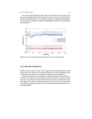
![98 4 ECG Signal Compression
4.4 R - Peak Detection
A basic task necessary for our electrocardiogram (ECG) compression algorithm is
the R wave peak detector. This task is necessary both for building the dictionary
used in the sparse representation phase and for the compression stage that they re-
quire RR signal bloks. To detect the peaks in ECG signals one can encounter some
difficulties, i.e. irregular peak form, irregular distance between peaks and presence
of low-frequency component due to patient breathing etc.
In literature many algorithms for QRS and R peak detection were presented. The
principal techniques are based on the filtering and thresholding of the signal [63, 89],
wavelets [36, 1] and template matching [30]. In our algorithm we use a simple and
inexpensive method to detect R peaks, that does not preserve information about the
Q and S waves, that are not useful for our purpose.
Let assume to have a digital ECG signal s = (s1,...,sn) ∈ Rn. The first step
in the ECG peak detection algorithm is to remove the low-frequency components.
We apply a direct Fast Fourier Transform (FFT), remove the low frequencies by
thresholding and reconstruct the ECG signal by applying the Inverse Fast Fourier
Transform (IFFT).
The second step is to find local maxima using a windowed nonlinear filter. This pro-
cess puts to zero all the values in the window except the local maximum.
The last step is to remove the small values that called false positives, i.e. high volt-
age T waves. To do this, we threshold the local maxima found in the previous step
with appropriate value that can be easily set equal to a percentage of the absolute
maximum of the signal s.
4.5 Compression Method
The algorithm for ECG signal compression and reconstruction is summarized in
Fig. 4.4. It consists of a block-wise sparse coding preceded by standard preprocess-
ing and dictionary creation, and followed by a final lossless compression of sparse
coefficients, as detailed in the following.
4.5.1 Dictionary Creation and Signal Normalization
The ECG signal s = (s1,...,sn) ∈ Rn
can be modeled as a mixture of two cardiac
activities:
s = sVA + sAA (4.1)](https://image.slidesharecdn.com/f546e914-990d-4b7e-af7b-78d9394c1be8-160713201804/85/phd_unimi_R08725-114-320.jpg)
![4.5 Compression Method 99
Preprocessing
Create the ECG
Sparse Encoding
s.t.
Coefficients
Normalization
Lossless
Compression
Dictionary Φ
minα||α||0
||Φα − s||2
2 ≤ ǫ
Fig. 4.4 Block diagram of the signal encoding phase.
where sAA ∈ Rn denotes the atrial activity signal and sVA ∈ Rn represent the ventric-
ular activity signal.
The generation of good sparse models for the atrial sAA and the ventricular sVA
signals requires the use of dictionaries capable to fit the signal structure.
The approach proposed in [40] is based on the decomposition of the ECG signal s
in a redundant dictionary Φ ∈ Rn×m that is a composition of two sub dictionaries:
ΦAA ∈ Rn×k1 suited for the representation of the atrial activity and ΦVA ∈ Rn×k2 able
to represent the ventricular activity (with m = k1 + k2).
In this way the ECG signal can be represented as
s = ΦVAαVA + ΦAAαAA (4.2)
The subdictionary ΦVA in [40] was proposed to be generated by all possible trans-
lations of the Generalized Gaussian function
gVA(t) = cexp(−
|t − a|d
b
) (4.3)
where c is a normalization constant, a represents the position, b is the scale and d
is the peakiness, conversely the subdictionary ΦAA was proposed to be generated by
all translations of the real Gabor function
gAA(t) = cexp −
t − a
b
2
cos
2πk(t − a)
n
− ∆θ (4.4)
where n is the signal length, a the peak position, c the normalization constant, b the
scale and ∆θ the phase.
In [75] was proposed to learn the subdictionaries from training samples by alter-
nating dictionary learning phases for ΦAA and ΦVA.](https://image.slidesharecdn.com/f546e914-990d-4b7e-af7b-78d9394c1be8-160713201804/85/phd_unimi_R08725-115-320.jpg)
![100 4 ECG Signal Compression
In [53, 30] ECG signals, were represented using a nlog2 n waveforms analytically
represented by wavelets functions (like the Haar, Coiflet4, Deaubuchies18, Battle3
and Symmlet8) as atoms of the dictionary Φ.
Alternative dictionaries are proposed in [61]. The first kind of dictionary, called
Resampled Cardiac Pattern, uses as atoms cardiac pattern taken between the middles
of successive RR intervals of the ECG signal. Each segment contains the P wave,
the QRS complex and the T wave. The second kind of overcomplete dictionary is
called Resampled R-centered Cardiac Patterns and is built taking beats patterns from
an ECG signal each of which is elastically shrinked and stretched with respect to the
peak of the R wave, until it is moved in the middle of the waveform.
Algorithm 5 Dictionary Creation
Require: - the ECG signal s
- the number m of atoms
- the length n of atoms
- the vector of peak positions RR
for i = 1,...,m do
2: µ =
RRi+1−RRi
2 < calculate the mean of the current RR interval >
sl = sRRi:(RRi+µ−1) < set the left half part of the current RR interval into sl >
4: sr = s(RRi+µ):(RRi+1−1) < set the right half part of the current RR interval into sr >
z = (0,...,0) ∈ Rn−(RRi+1−RRi) < create the zero padding vector >
6: φi = [sT
l ,zT ,sT
r ]T < stretch the atom to the fixed size >
end for
8: return Φ = {φ1,...,φm} < the dictionary Φ >
Following the idea in [61] to use natural patterns as representation basis of the
ECG signal, in our algorithm we propose a dictionary constructed from pieces of
RR interval sampled from the ECG signal that we want to compress. Given an ECG
signal, an overcomplete dictionary is built using the cardiac patterns of the signal
extracted from an initial transitory of few seconds’ duration. To do this, the signal
is segmented by taking patterns between successive RR intervals. Each segment s
contains two halves of the QRS complex with the T-wave on the left and the P-wave
on the right. s is then normalized extending its length to the size of the sample rate
by adding the right number of zeros in the middle.
The normalization meaning is obviously that of concentrating the distribution or
RR-peaks at the extrema of each segment in order to facilitate the sparse represen-
tation stage. In fact, the more the signal is regular and closer to be a cyclostationary
process, the higher the sparse representation will be. Thus, the light overhead given
by the normalization phase is widely compensated by the high level of sparsity
that could be potentially reached. This stage should then imply a first significant](https://image.slidesharecdn.com/f546e914-990d-4b7e-af7b-78d9394c1be8-160713201804/85/phd_unimi_R08725-116-320.jpg)
![4.5 Compression Method 101
numerosity reduction of coefficients involved in the sparse representation and con-
sequently a first decisive step toward high compression ratio.
100 200 300 400 500
−500
0
500
100 200 300 400 500
−500
0
500
100 200 300 400 500
−500
0
500
Fig. 4.5 Example of atoms from the original signal s. In red the zero padding for atom length
normalization.
After normalization, taken a set of m heart-beat segments φi (i = 1...,m) of size
n, with n < m, the dictionary Φ is obtained stacking all basis vectors (or atoms)
so that Φ = [φ1,...,φm], represents a linear mapping into a suitable feature space
S ⊆ Rn. This algorithm is summarized in Algorithm (5). Each atom of the dic-
tionary Φ so builted, ensures to represent the clinical information such as the PR
interval, the P wave configuration, the RR duration etc.
4.5.2 Sparse Representation
The main purpose of the sparsity promotion phase is to adaptively choose the spar-
sity level k in order to guarantee an upper bound on the discrepancy between the
i-th ECG segment si and its sparse representation ˆsi. To this end we introduce the
main criterion involved in such approximation in order to respect the bounded error
requirement, namely the Percent Root-Mean Square Difference (PRD) defined as:](https://image.slidesharecdn.com/f546e914-990d-4b7e-af7b-78d9394c1be8-160713201804/85/phd_unimi_R08725-117-320.jpg)

![4.5 Compression Method 103
4.5.3 Quantization and Compression
For long term signal of N heart-beats the data we have to compress are of three
kinds:
1. the set of coefficients (amended by zeros elements) contained in the vectors
α1,...,αN whose number amount to K = ∑N
i=1 ki. Fixed q bits for 2q quanti-
zation levels we simply rescale and quantize each coefficient c into the integer
number
cq = round
c− αmin
αmax − αmin
(2q
− 1) (4.6)
where αmin and αmax are the minimum and maximum value coefficients.
2. Once processed coefficients, we have to compress the positions of coefficients
different from zero, i.e., the characteristic vectors {χα1,...,χαN }, one for each
n-tuple αi, identifying the positions of coefficients not null. The concatenation
of the binary vectors χαi forms a sparse bit-vector with K ones over nN bits,
with K ≪ nN. An effective way to compress them is to use of Huffman coding
[65] for bit-vectors. It is partitioned into blocks of fixed size l and statistics are
collected on the frequency of occurrence of the 2l bit patterns. Based on these
statistics the set of blocks is Huffman encoded and the bitmap itself is encoded
as a sequence of such codewords For sparse vectors the l-bit block consisting
of zeros only and blocks with only a single 1-bit have much higher probabilities
than the other blocks so the average codeword length of the Huffman code will
be smaller than l.
3. The last set of numbers ρ1,...,ρN to be compressed are those involved in the
zero-padding normalization task, accomplished for each heart-beat. An effec-
tive way to encode such a list is with the delta encoding, which stores the dif-
ferences between pairs of successive values in the list. Such encoding is par-
ticularly useful in our case where most of the differences are small. The final
sequence of differences can be thus compressed much more efficiently by most
of the compression algorithms.
Restore
Coefficients
DecodingSparse
Decompression
Lossless
ˆs = Φα
Fig. 4.6 Block diagram of the signal reconstruction phase.](https://image.slidesharecdn.com/f546e914-990d-4b7e-af7b-78d9394c1be8-160713201804/85/phd_unimi_R08725-119-320.jpg)
![104 4 ECG Signal Compression
4.6 Performance Evaluation
The compression performances for a cardiac signal x of fixed duration is computed,
as usual, in terms of Compression Ratio (CR) [102]:
CR =
# bits of x
# bits of ˆx
.
In our setting the signal to be compressed is a sequence of N cardiac segments x =
[s1,...,sN] picked sequentially by a sliding window without overlapping. As already
mentioned in the previous section, to accomplish this task we have to compress three
kinds of data: not null coefficients in each vectors αi, characteristic bit-vectors χi
and padding numbers ρi. Putting all tighter, the CR thus becomes
CR =
N × fs × 11
Bα + Bχ + Bρ
,
where fs the sampling frequency and Bα, Bχ, Bρ the number of bits coding coeffi-
cients, characteristic vectors and padding numbers respectively.
However, in the case of lossy data compression, the data compression ratio does
not provide sufficient detail on the performances because it does not reflect distinc-
tion between the original signal and the reconstructed signal.
Regarding the error, since PRD [6] measure heavily depends on the mean value
¯s of the ECG signal s, it is sometime more suitable to use the normalized PRD
measure given by
PRDN = 100
s− ˆs
s− ¯s
.
where ¯s is the mean value of the signal s.
Another measure typically used to evaluate the reconstruction error is the root
mean square error (RMS) defined as
RMS =
1
n
||s− ˆs||2
2 (4.7)
where n is the length of the window over which the RMS is evaluated [126].
The RMS quantifies the amount of the original signal discarded by the compression
method, as measured by the difference between the signal s and ˆs.
An important aspect of performanceevaluation is the choice of the ECG database.
As the performance of a method depends on the noise level, the evaluation should
be based on data representative of the application of interest.
In the next session we describe the PhysioNet MIT-BIH Arrhythmia database [59],
used to evaluate the performances of our algorithm.](https://image.slidesharecdn.com/f546e914-990d-4b7e-af7b-78d9394c1be8-160713201804/85/phd_unimi_R08725-120-320.jpg)
![4.8 Experimental Results 105
4.7 PhysioNet MIT-BIH Arrhythmia Database
PhysioNet offers free web access to large collections of recorded physiologic sig-
nals (PhysioBank) and related open-source software (PhysioToolkit) [59].
Since 1975 the Massachusetts Institute of Technology (MIT) together with the Beth
Israel Deaconess Medical Center have carried out research concerning medical ex-
aminations analysis and related points.
One of the first major product of that effort was the MIT-BIH Arrythmia database
(downloadable from the PhysioNet web site [59]) which was completed in 1980.
This database contains standard test material for evaluation of arrythmia detectors.
The MIT-BIH Arrhythmia Database contains 48 half-hour excerpts of two-
channel ambulatory ECG recordings, obtained from 47 subjects studied by the BIH
Arrhythmia Laboratory between 1975 and 1979. Twenty-three recordings were cho-
sen random from a set of 4000 24-hour ambulatory ECG recordings collected from a
mixed population of inpatients (about 60%) and outpatients (about 40%) at Boston’s
Beth Israel Hospital; the remaining 25 recordings were selected from the same set to
include less common but clinically significant arrhythmias that would not be well-
represented in a small random sample.
The recordings were digitized at 360 samples per second per channel with 11-bit
resolution over a 10 mV range and each signal was independently annotated from
two or more cardiologists.
4.8 Experimental Results
In order to evaluate the compression performances of the k-LIMAPS based com-
pression algorithm, we have performed extended computer simulations. Tests were
conducted using the records 100, 101, 102, 109, 111, 112, 113, 115, 117, 119 and
121 extracted from the MIT-BIH Arrythmia database [63]. These signals are 30
minutes registrations sampled at 11 bits with a sampling rate of 360 Hz.
Each recording was splitted in two parts: the first one of about 10 minutes, used
for the dictionary creation phase, the second one for the sparse representation and
signal compression.
Our experiments were performed on an AMD Athlon II X4 630 Processor 64 bit,
2.8 GHz processor with 4 GB of memory, implementing our algorithm in MATLAB
v.2011b.
In table (4.1) we can see results for the compression of the selected records. Each
one is quantized with two different quantization rate: 6 and 7 bits. With the 6 bits](https://image.slidesharecdn.com/f546e914-990d-4b7e-af7b-78d9394c1be8-160713201804/85/phd_unimi_R08725-121-320.jpg)

![4.8 Experimental Results 107
0 1 2 3 4 5
900
1000
1100
1200
(b)
0 1 2 3 4 5
−150
−100
−50
0
50
100
150
(c)
0 1 2 3 4 5
900
1000
1100
1200
(a)
Fig. 4.7 Compression of the record 100 with CR = 75.12 and PRD = 0.68. (a) Original signal. (b)
Reconstructed signal. (c) Error signal.
In table (4.3) we summarize comparative results with the algorithms DCeq-MMP
[52] (Multididimensional Multiscale Parser) and with Foveation [33] + SPIHT algo-
rithm (Set Partitioning in Hierarchical Trees [101, 106]) for records 100, 102, 115,
117 and 119.
In all the experiments conducted, the PRD of each signal was calculated with
respect to the original non-processed signal mean. This turns out to be necessary
because different preprocessing filtering can change significantly the average signal
magnitude, making the results incomparable.
As we can see for almost all the records, the compression rate obtained by our
algorithm is the highest, maintaining a PRD less or comparable to other algorithms.
An exception is found for the record 119: in this case this the irregularities of the
RR interval and the presence of large muscular noise, the atoms of the dictionary do
not represent properly the signal when only few coefficients are adopted.](https://image.slidesharecdn.com/f546e914-990d-4b7e-af7b-78d9394c1be8-160713201804/85/phd_unimi_R08725-123-320.jpg)
![108 4 ECG Signal Compression
Table 4.3 Performance comparison of different ECG compression schemes
Method Record CR PRD
DCeq - MMP [52] 100 24 3.30
Foveation + SPIHT [33] 100 20 0.52
k-LIMAPS (7 bit) 100 74.12 0.68
k-LIMAPS (6 bit) 100 78.20 0.72
DCeq - MMP [52] 102 10 2.03
k-LIMAPS (7 bit) 102 48.47 0.68
k-LIMAPS (6 bit) 102 50.54 0.69
DCeq - MMP [52] 115 30.6 2.92
k-LIMAPS (7 bit) 115 36.57 0.61
k-LIMAPS (6 bit) 115 38.26 0.65
DCeq - MMP [52] 117 13 0.91
Foveation + SPIHT [33] 117 32 0.51
k-LIMAPS (7 bit) 117 37.13 0.56
k-LIMAPS (6 bit) 117 38.19 0.61
DCeq - MMP [52] 119 20 1.83
DCeq - MMP [52] 119 10 1.07
DCeq - MMP [52] 119 8 0.91
Foveation + SPIHT [33] 119 20 0.49
k-LIMAPS (7 bit) 119 15.24 1.90
k-LIMAPS (6 bit) 119 16.26 3.74
4.9 Garanteed-Percentage Root Mean Square Difference Error
In this section we present a variant of the ECG compression algorithm explained in
4.5. The main difference concerns the dictionary construction: in this variant it is a
concatenation of two dictionaries, one extracted directly from a portion of the signal
to be compressed, the second is a random generated matrix used with the purpose of
improving the ability of sparse recovery of k-LIMAPS into a natural base. Moreover
no zero padding is added to the natural signals, thus no noise in the superposition
of atoms are added and propagated to the compressed coefficients. The algorithm
proposed in this section ensures that the recovered signal has a guaranteed PRD
error.](https://image.slidesharecdn.com/f546e914-990d-4b7e-af7b-78d9394c1be8-160713201804/85/phd_unimi_R08725-124-320.jpg)
![4.9 Garanteed-Percentage Root Mean Square Difference Error 109
4.9.1 Dictionary Creation
The dictionary is created by slicing a natural ECG signal with a fixed window size.
Atoms are selected as non overlapped pieces of signal that contain (in average) only
one beat. To do this, in the case the ECG signal used, belongs to subjects at rest, we
can simply choose a window size of dimension approximately equal to the sampling
rate. This assumption is justified by the fact that in normal conditions, the average
heart beat rate is in the interval of 60-80 bpm (beat per minute). If an estimate of
the average beats per minutes is available, another possible choice for the temporal
resolution is given by the formula
tr = ⌈
abpm
60
∗ fs⌉
where abpm is the average beat per minutes and fs is the sampling rate frequency.
0 50 100 150 200 250
−100
−50
0
50
100
150
200
250
300
ECG Dictionary Atoms
Fig. 4.8 Example of Dictioanry Atoms.
In figure 4.8 we can see examples of dictionary atoms extracted by slicing the
ECG signal with a temporal resolution equal to the sampling rate.
A generalization of the notion is presented in [8], where two fundamental mea-
sures of coherence are introduced: worst-case coherence and the average coherence
, among the columns of a matrix.
Let Φ be an n × m matrix with unitary norm columns φi ∈ Rn, [8] defines](https://image.slidesharecdn.com/f546e914-990d-4b7e-af7b-78d9394c1be8-160713201804/85/phd_unimi_R08725-125-320.jpg)
![110 4 ECG Signal Compression
µ(Φ) = max
i,j:i= j
| < φi,φj > | (4.8)
ν(Φ) =
1
m− 1
max
i
| ∑
j:j=i
< φi,φj > | (4.9)
respectively the worst-case coherence and the average coherence of Φ. The smaller
the worst-case coherence, the less similar the columns. On the other hand, the av-
erage coherence is a measure of the spread of the columns of a dictionary matrix
within the n-dimensional unit ball. TNote that, in addition to having zero worst-case
coherence, orthonormal bases also have zero average coherence.
The uniqueness of the sparsest solution of an underdetermined linear system de-
pends on the worst-case coherence of the dictionary Φ. Recalling the theorem 1.3:
i f a linear system Φα = s has a solution α such that ||α||0 < 1
2 (1 + 1
µ(Φ) ), than
α is the sparsest solution. Futhermore, the worst case analysis tells us that we can
recover superposition of k atoms as long as
k
1
µ(Φ)
≈
√
m (4.10)
The resulting worst case bounds for recoverable sparsity levels turn out to be overly
pessimistic and quite in contrast to the much better performancearchived in practice.
The natural bases extracted from the ECG signal, does not guarantee a low worst
case coherence, making difficult to recover the sparsest solution of the underdeter-
mined system.
It was established in [8] that when the average coherence ν(Φ) is sufficiently
smaller than µ(Φ), a number of guarantees can be provided for sparse signal pro-
cessing.
To decrease the average coherence of our dictionary, we concatenate the dictio-
nary containing atoms extracted from natural ECG signal with a dictionary random
sampled from a Gaussian distribution.
Formally let Φ be the dictionary created by segmenting the natural ECG signal,
and let Ψ be the dictionary sampled from a Gaussian distribution N (0, 1
n ), we can
recast the regularization problem 4.5 as
min
αi∈Rm
αi 0 subject to PRD(si,Σαi) ≤ PRDmax, (4.11)
with Σ defined as
Σ = [Φ|Ψ]
that is the concatenation of the two dictionaries.
As proved in [8], we note that the average coherence of Gaussian matrix Ψ ∈
Rn×p
with i.i.d. N (0, 1
n ) entries, is
ν(Ψ) ≤
√
15log p
n](https://image.slidesharecdn.com/f546e914-990d-4b7e-af7b-78d9394c1be8-160713201804/85/phd_unimi_R08725-126-320.jpg)
![4.9 Garanteed-Percentage Root Mean Square Difference Error 111
200 400 600 800 1000 1200 1400 1600 1800
50
100
150
200
250
300
350
ECG Atoms
Random Atoms
Fig. 4.9 ECG Dictionary with Gaussian atoms. The left part of the dictionary contains atoms
sampled from ECG signal, right part are atoms random sampled from Gaussian distribution.
with probability exceeding 1 − 2p−2 as long as p > n ≥ 60log p.
Conversely, the dictionary Φ extracted by natural ECG signal has a high average
coherence, hence concatenating the two dictionaries we can establish the following
relation
ν(Ψ) ≤ ν(Σ) ≤ ν(Φ)
4.9.2 Experimental Results
To analyze the compression performances of the method described in this session,
we have performed a wide range of experiments using the records taken from the
MIT-BIH Arrythmia database [63], as we have done to evaluate the k-LIMAPS
ECG in section 4.5.
Each record signal was divided in two partitions: one of about 12 minutes for the
creation of the subdictionary, and the other to be used to measure the compression
capability of the method.
In table (4.4) we resume the results of compression performances reached by the
Garanteed-Percentage Root Mean Square Difference Error algorithm, obtained over
a selection of ECG records taken from the MIT-BIH Arrythmia database.](https://image.slidesharecdn.com/f546e914-990d-4b7e-af7b-78d9394c1be8-160713201804/85/phd_unimi_R08725-127-320.jpg)


![Appendix A
MATLAB Code
A.1 LIMAPS
function [ alpha ] = LiMapS(s, D, DINV, gamma, maxIter, ftype)
%
% [ alpha ] = LIMAPS(s, D, DINV, gamma, maxIter, ftype)
%
% Returns the sparsest vector alpha which satisfies underdetermined
% system of equations D*alpha=s, using Lipschitzian Mapping for Sparsity
% Recovery algorithm.
% The dictionary matrix D should have more columns than rows. The
% number of rows of dictionary D must be equal to the length of the
% column observation vector(or matrix) s.
%
% The observations signal(s) s and the dictionary D necessarily, must
% be provided by the user. The other parameters have defult values, or
% may be provided by the user.
%
% This algorithm work fine with matrix too, returning the sparsest matrix
% alpha that satisfy the underdetermined system of equations D*alpha=s.
% Then the dictionary D is of size [n x m], s must be of size [ s x T ] and
% as consiquence the coefficients matirx alpha is of size [ m x T]
%
% s:
% The observation vector (matrix)
%
% D:
% The dictionary
%
% DINV (optional):
% The pseudo-inverse of the dictionary matrix D
%
% gamma (optional):
% The increase factor (default 1.01)
%
115](https://image.slidesharecdn.com/f546e914-990d-4b7e-af7b-78d9394c1be8-160713201804/85/phd_unimi_R08725-131-320.jpg)

![A.1 LIMAPS 117
% choose the shrinking function
f=shrinkage_function (ftype);
%% -- CORE --
for i=1:maxIter
alphaold=alpha;
% apply sparsity constraction mapping: increase sparsity
beta = f(alpha,lambda);
beta(abs(beta)<alpha_min)=0;
% apply the orthogonal projection
alpha = beta-DINV*(D*beta-s);
% update the lambda coefficient
lambda = lambda*gamma;
% check the stopping criteria
if (norm(alpha(:)-alphaold(:))<epsilon)
break;
end
if (mod(i,100))
if(sum(abs(f(alpha,lambda)./alpha)>1/lambda)>size(D,1))
break;
end
end
end
%% -- REFINEMENT --
% threshold the coefficients
alpha(abs(alpha)<alpha_min) = 0;
% final refinements of the solution
for i=1:size(alpha,2);
alpha_ind = alpha(:,i)=0;
D1 = D(:,alpha_ind);
alpha(alpha_ind,i) = alpha(alpha_ind,i) - pinv(D1)*(D1*alpha(alpha_ind,i)-s(:,i));
end
end
function [ f ] = shrinkage_function ( type )
f = @exponential_func;
switch(type)
case 'exp'
f = @exponential_func;
case 'exp2'
f = @exponential2_func;](https://image.slidesharecdn.com/f546e914-990d-4b7e-af7b-78d9394c1be8-160713201804/85/phd_unimi_R08725-133-320.jpg)
![118 A MATLAB Code
case 'htan'
f = @hyperbolic_tangent_func;
case 'abs'
f = @absolute_value_func;
case 'sqrt'
f = @square_root_func;
case 'err'
f = @error_func;
case 'gud'
f = @gudermannian_func;
end
end
function [ y ] = exponential_func(x,lambda)
y=x.*(1-exp(-lambda*abs(x)));
end
function [ y ] = exponential2_func(x,lambda)
y=x.*(2./(1+exp(-lambda*abs(x)))-1);
end
function [ y ] = hyperbolic_tangent_func(x,lambda)
y=x.*tanh(lambda*abs(x));
end
function [ y ] = absolute_value_func(x,lambda)
y=x.*(lambda*x.ˆ2./(1+lambda*x.ˆ2));
end
function [ y ] = square_root_func(x,lambda)
y=x.*(lambda*abs(x))./sqrt(1+(lambda*x).ˆ2);
end
function [ y ] = error_func(x,lambda)
y=x.*erf(lambda*abs(x));
end
function [ y ] = gudermannian_func(x,lambda)
y=x.*(2/pi*atan(sinh(pi/2*lambda*abs(x))));
end
A.2 k-LIMAPS
function [ alpha ] = KLiMapS(s, D, k, DINV, maxIter, ftype)
%
% [ alpha ] = KLIMAPS(s, D, k, DINV, maxIter, ftype)
%
% Returns the k-sparse vector alpha which satisfies underdetermined
% system of equations D*alpha=s, using Lipschitzian Mapping for Sparsity
% Recovery algorithm.
% The dictionary matrix D should have more columns than rows. The](https://image.slidesharecdn.com/f546e914-990d-4b7e-af7b-78d9394c1be8-160713201804/85/phd_unimi_R08725-134-320.jpg)
![A.2 k-LIMAPS 119
% number of rows of dictionary D must be equal to the length of the
% column observation vector(or matrix) s.
%
% The observations signal(s) s and the dictionary D necessarily, must
% be provided by the user. The other parameters have defult values, or
% may be provided by the user.
%
% This algorithm work fine with matrix too, returning the sparsest matrix
% alpha that satisfy the underdetermined system of equations D*alpha=s.
% Then the dictionary D is of size [n x m], s must be of size [ s x T ] and
% as consiquence the coefficients matirx alpha is of size [ m x T]
%
% s:
% The observation vector (matrix)
%
% D:
% The dictionary
%
% k:
% Number of coefficients to select
%
% DINV (optional):
% The pseudo-inverse of the dictionary matrix D
%
% gamma (optional):
% The increase factor (default 1.01)
%
% maxIter (optional):
% Maximum number of iterations (default 1000)
%
% ftype (optional):
% String that represent the shrinking function
% - 'exp' (default) exponential
% - 'exp2' exponential function
% - 'htan' hyperbolic function
% - 'abs' absolute value function
% - 'sqrt' square root function
% - 'err' error function
% - 'gud' Gudermannian function
%
% Authors: Alessandro Adamo and Giuliano Grossi
% Version: 1.0
% Last modified: 1 Aug. 2011.
%
% WEB PAGE:
% ------------------
% http://dalab.dsi.unimi.it/klimaps
%
% HISTORY:
%--------------
% Version 2.0: 9 Feb. 2013
% official version.
%
if(nargin<3||nargin>6)](https://image.slidesharecdn.com/f546e914-990d-4b7e-af7b-78d9394c1be8-160713201804/85/phd_unimi_R08725-135-320.jpg)

![A.2 k-LIMAPS 121
end
function [ f ] = shrinkage_function ( type )
f = @exponential_func;
switch(type)
case 'exp'
f = @exponential_func;
case 'exp2'
f = @exponential2_func;
case 'htan'
f = @hyperbolic_tangent_func;
case 'abs'
f = @absolute_value_func;
case 'sqrt'
f = @square_root_func;
case 'err'
f = @error_func;
case 'gud'
f = @gudermannian_func;
end
end
function [ y ] = exponential_func(x,lambda)
y=x.*(1-exp(-lambda*abs(x)));
end
function [ y ] = exponential2_func(x,lambda)
y=x.*(2./(1+exp(-lambda*abs(x)))-1);
end
function [ y ] = hyperbolic_tangent_func(x,lambda)
y=x.*tanh(lambda*abs(x));
end
function [ y ] = absolute_value_func(x,lambda)
y=x.*(lambda*x.ˆ2./(1+lambda*x.ˆ2));
end
function [ y ] = square_root_func(x,lambda)
y=x.*(lambda*abs(x))./sqrt(1+(lambda*x).ˆ2);
end
function [ y ] = error_func(x,lambda)
y=x.*erf(lambda*abs(x));
end
function [ y ] = gudermannian_func(x,lambda)
y=x.*(2/pi*atan(sinh(pi/2*lambda*abs(x))));
end](https://image.slidesharecdn.com/f546e914-990d-4b7e-af7b-78d9394c1be8-160713201804/85/phd_unimi_R08725-137-320.jpg)

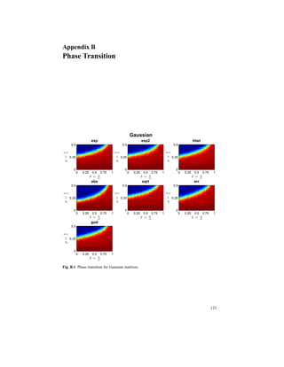


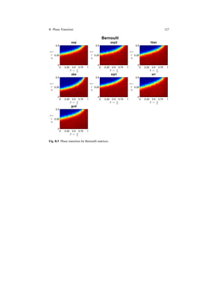
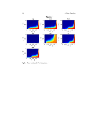
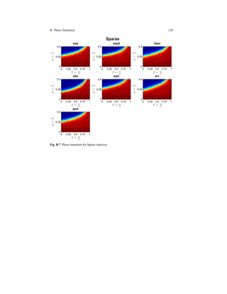

![References 131
References
1. Wavelets for QRS detection, volume 2, November 2002.
2. Alessandro Adamo and Giuliano Grossi. A fixed-point iterative schema for error minimiza-
tion in k-sparse decomposition. pages 167–172, 2011.
3. Alessandro Adamo, Giuliano Grossi, and Raffaella Lanzarotti. Sparse representation based
classification for face recognition by k-limaps algorithm. In ICISP, pages 245–252, 2012.
4. P. S. Addison. Wavelet transforms and the ECG: a review. Physiol Meas, 26(5), October
2005.
5. M. Aharon, M. Elad, and A. Bruckstein. K-SVD: An Algorithm for Designing Overcom-
plete Dictionaries for Sparse Representation. Signal Processing, IEEE Transactions on,
54(11):4311–4322, November 2006.
6. Sabah M. Ahmed, Anwer Al-Shrouf, and Mohammed Abo-Zahhad. ECG data compression
using optimal non-orthogonal wavelet transform. Medical engineering & physics, 22(1):39–
46, 2000.
7. K. Ayarpadi, E. Kannan, R. R. Nair, T. Anitha, R. Srinivasan, and P.G. Scholar. Face Recogni-
tion under Expressions and Lighting Variations using Masking and Synthesizing. 2(1):758–
763, 2012.
8. Waheed U. Bajwa, A. Robert Calderbank, and Sina Jafarpour. Why gabor frames? two fun-
damental measures of coherence and their role in model selection. CoRR, abs/1006.0719,
2010.
9. S. Banach. Th´eorie des op´erations lin´eaires. Varsovie, 1932.
10. Stefan Banach. Sur les op´erations dans les ensembles abstraits et leur application aux
´equations int´egrales. Fundamenta Mathematicae III, pages 133–181, 1922.
11. BANCA DB. Address:
http://www.ee.surrey.ac.uk/Research/VSSP/banca/. web.
12. Richard Baraniuk, Mark Davenport, Ronald DeVore, and Michael Wakin. A Simple Proof
of the Restricted Isometry Property for Random Matrices. Constructive Approximation,
28(3):253–263, 2008.
13. Amir Beck and Marc Teboulle. A fast iterative shrinkage-thresholding algorithm for linear
inverse problems. SIAM J. Img. Sci., 2(1):183–202, March 2009.
14. P.N. Belhumeur, J.P. Hespanha, and D.J. Kriegman. Eigenfaces vs. Fisherfaces: Recognition
using class specific linear projection. IEEE Trans. Pattern Analysis and Machine Intelligence,
19(7):711–720, 1997.
15. Jeffrey D. Blanchard, Coralia Cartis, and Jared Tanner. Compressed sensing: How sharp is
the restricted isometry property? SIAM Review, 53(1):105–125, 2011.
16. Jeffrey D. Blanchard, Coralia Cartis, Jared Tanner, and Andrew Thompson. Phase transitions
for greedy sparse approximation algorithms. CoRR, abs/1004.1821, 2010.
17. Thomas Blumensath. Accelerated iterative hard thresholding. Signal Processing, 92(3):752–
756, 2012.
18. P. Campadelli, R. Lanzarotti, and G. Lipori. Automatic facial feature extraction for face
recognition. In Delac and Grgic [37], pages 31–58.
19. P. Campadelli, R. Lanzarotti, and G. Lipori. Precise eye and mouth localization. International
Journal of Pattern Recognition and Artificial Intelligence, 23(3), 2009.
20. E. J. Cand`es. The restricted isometry property and its implications for compressed sensing.
Comptes Rendus Mathematique, 346(9-10):589–592, may 2008.
21. E. J. Candes, J. Romberg, and T. Tao. Robust uncertainty principles: exact signal reconstruc-
tion from highly incomplete frequency information. Information Theory, IEEE Transactions
on, 52(2):489–509, February 2006.
22. E. J. Candes and T. Tao. Decoding by Linear Programming. IEEE Transactions on Informa-
tion Theory, 51(12):4203–4215, December 2005.
23. E. J. Candes and T. Tao. Near-Optimal Signal Recovery From Random Projections: Uni-
versal Encoding Strategies? Information Theory, IEEE Transactions on, 52(12):5406–5425,
December 2006.](https://image.slidesharecdn.com/f546e914-990d-4b7e-af7b-78d9394c1be8-160713201804/85/phd_unimi_R08725-147-320.jpg)