Downloaded 302 times


![Prince George’s Community College General Physics I D.G. Simpson
Figure 8.1: Vertical vs. horizontal motion. If two objects are released simultaneously (one falling vertically
and one given an initial horizontal velocity), then they both land on the floor at the same time. (Ref. [9])
For the second ball (the one given an initial horizontal velocity v0), we have a D g j, v0 D v0 i, and r0 D 0;
therefore
r.t/ D 1
2
at2
C v0t C r0 (8.29)
D v0t i 1
2 gt2
j (8.30)
or
x.t/ D v0t (8.31)
y.t/ D 1
2
gt2
: (8.32)
So both balls have the same vertical (y) component of motion. Both balls fall together vertically, but the sec-
ond ball has a uniform horizontal motion superimposed on its vertical motion; the combination of horizontal
and vertical motions gives the second ball a parabolic path, as we’ll see in Chapter 9.
8.7 Summary
Let’s summarize the results so far for two- and three-dimensional kinematics:
Always True
These equations are definitions, and are always true:
v D
dr
dt
) r.t/ D
Z
v.t/ dt (8.33)
a D
dv
dt
D
d2
r
dt2
) v.t/ D
Z
a.t/ dt (8.34)
49](https://image.slidesharecdn.com/generalphysics-150426072326-conversion-gate01/75/General-physics-50-2048.jpg)


![Chapter 10
Newton’s Method
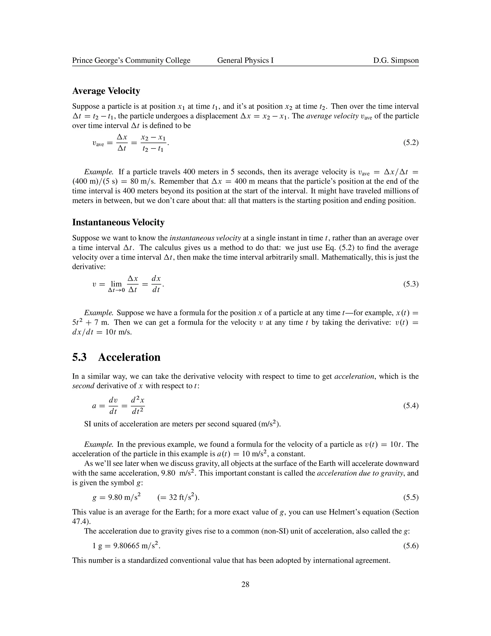
10.1 Introduction
As we have seen in the study of projectile motion, some problems in physics result in equations that cannot
be solved in closed form, but must be solved numerically. The study of the methods of solving such problems
is the field of numerical analysis, and is a course in itself. Here we look at one very simple method for
numerically finding the roots of equations, called Newton’s method.
10.2 The Method
Newton’s method is a numerical method for finding the root(s) x of the the equation
f .x/ D 0: (10.1)
The method requires that you first make an initial estimate x0 of the root. From that initial estimate, you
calculate a better estimate using the formula
xnC1 D xn
f .xn/
f 0.xn/
(10.2)
Applying this formula (with n D 0) to the initial estimate x0 gives a better estimate x1. This better estimate
x1 is then run through the formula again (n D 1) to get an even better estimate x2, etc. The process may be
repeated indefinitely to yield a solution to whatever accuracy is desired.
If the equation f .x/ D 0 has more than one root, then the method will generally find the one closest to
the initial estimate. Choosing different initial estimates closer to the other roots will find those other roots.
If there is no root (for example, f .x/ D x2
C 1 D 0), the method will tend to “blow up”: instead of
converging to a solution, you may just get bigger and bigger numbers, or you may get a series of different
numbers that show no sign of converging to a single value.
10.3 Example: Square Roots
When the first electronic calculators became available in the mid-1970s, many of them were simple “four-
function” calculators that could only add, subtract, multiply, and divide. The author’s father, L.L. Simpson
(Ref. [11]), showed him how he could calculate square roots on one of these calculators using Newton’s
method, as described here.
60](https://image.slidesharecdn.com/generalphysics-150426072326-conversion-gate01/75/General-physics-61-2048.jpg)


![Chapter 15
Atwood’s Machine
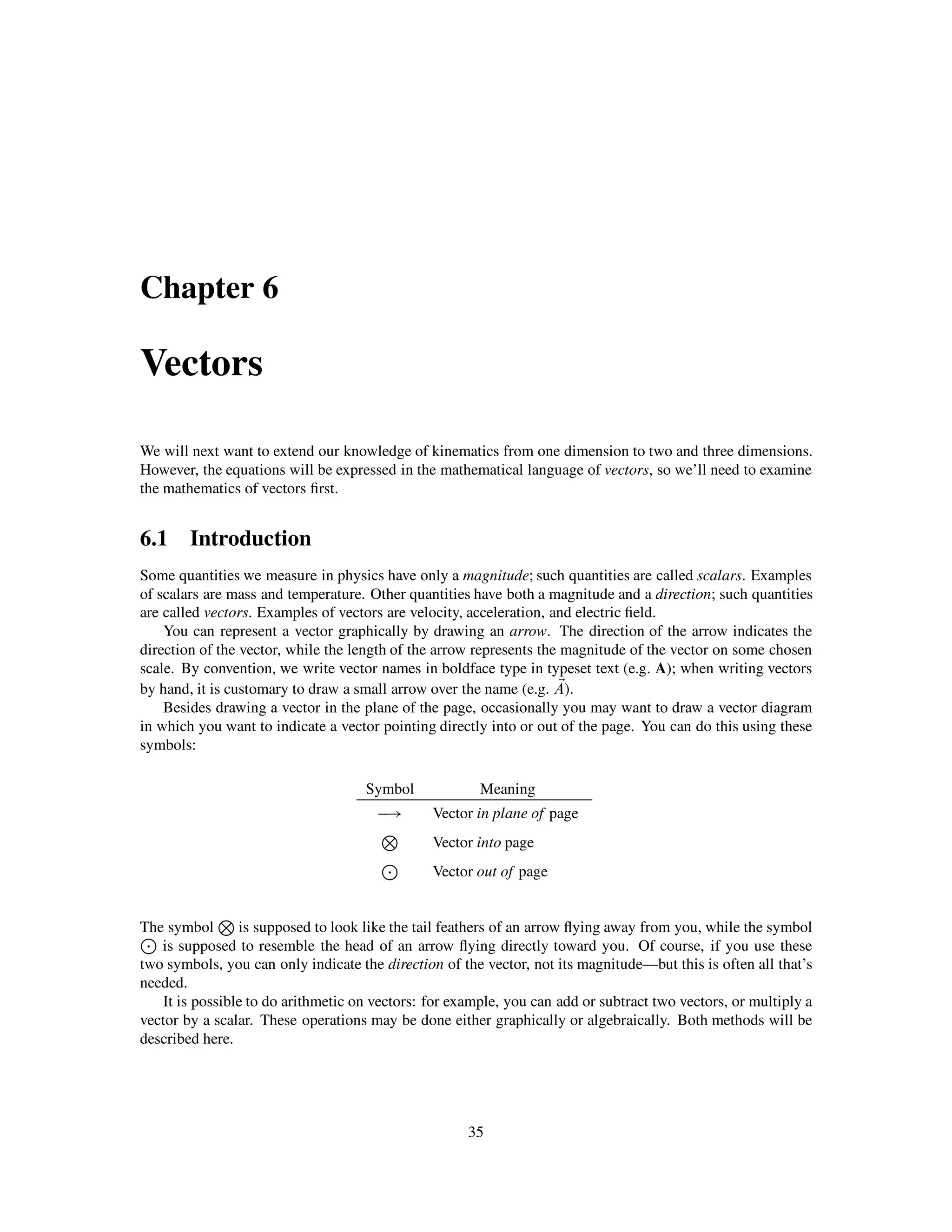
Figure 15.1: Atwood’s machine (Ref. [3]).
Atwood’s machine is a device invented in 1784 by
the English physicist Rev. George Atwood. (See
Fig. 15.1 at right.) The purpose of the device is
to permit an accurate measurement the acceleration
due to gravity g. In the 18th century, without accu-
rate timepieces or photogate timers, this was a diffi-
cult measurement to make with good accuracy. At-
wood’s machine has the effect of essentially scaling
g to a smaller value, so the masses accelerate more
slowly and allow g to be determined more easily.
Let’s see how the machine works. There are
two identical masses (labeled A and B in the fig-
ure) connected by a light string that is strung over
a pulley. Since the masses are identical, they will
not move, regardless of whether one is higher than
the other. The tall ( 8 ft) vertical pole has a distance
scale marked off in inches.
To use the machine, we move mass A to the top
of the scale, and place a small U-shaped bar on top
of the mass. (The bar is labeled M in the figure, but
is shown somewhat enlarged; the actual bar would
be just a little longer than the diameter of the ring.)
Now mass A will begin accelerating downward until
it reaches ring R. The mass will then pass through
ring R, but the ring will lift the bar off the mass,
so that the bar is left behind, sitting on the ring—in
effect, the ring “locks in” the final post-acceleration
velocity. After A passes through the ring, the masses
on both ends of the string will be the same, so the
acceleration will be zero and mass A will continue
moving with a constant velocity until it lands on
stage S. Both ring R and stage S are movable, and
can be moved up and down the scale as needed.
To collect data, we use a pendulum as a timing
device. Move ring R up and down until it takes one
69](https://image.slidesharecdn.com/generalphysics-150426072326-conversion-gate01/75/General-physics-70-2048.jpg)


![Prince George’s Community College General Physics I D.G. Simpson
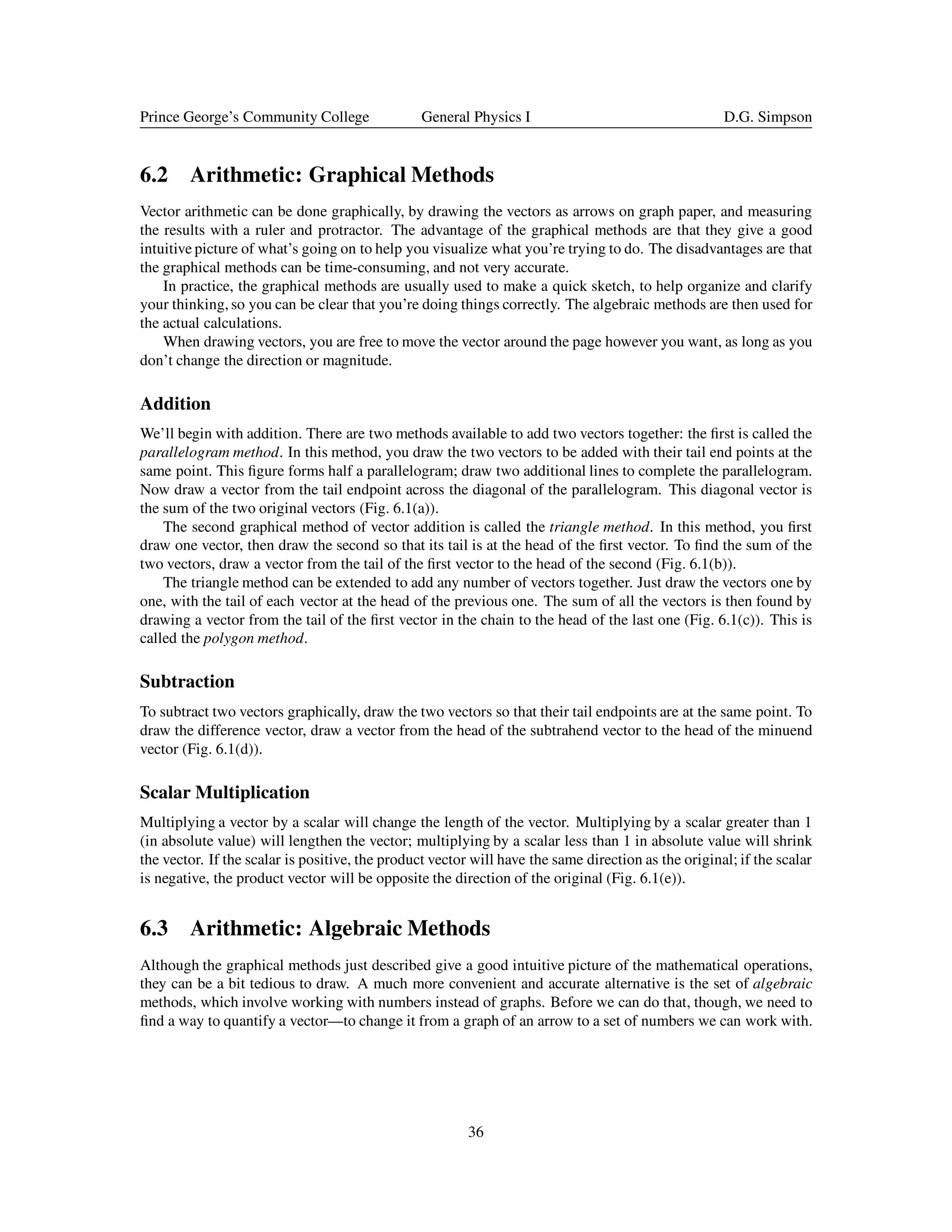
This is a first-order differential equation, which you will learn to solve for v.t/ in a course on differential
equations. But briefly, for a differential equation of the form
dy
dt
C p.t/y D q.t/; (18.6)
the solution y.t/ is found to be (Ref. [2])
y.t/ D
1
.t/
ÄZ
.t/ q.t/ dt C C ; (18.7)
where C is a constant that depends on the initial conditions, and .t/ is an integrating factor, given by
.t/ D exp
ÄZ
p.t/ dt : (18.8)
Since this is a first-order differential equation, there will be one arbitrary constant of integration, and it is the
constant C in Eq. (18.7).
Comparing Eq. (18.5) with Eq. (18.6), we have
y.t/ D v.t/; (18.9)
p.t/ D b=m; (18.10)
q.t/ D g: (18.11)
Then the integrating factor .t/ is, from Eq. (18.8),
.t/ D exp
ÄZ
p.t/ dt (18.12)
D exp
ÄZ
b
m
dt (18.13)
D Aebt=m
; (18.14)
where A is a constant of integration. The solution to Eq. (18.5) is then given by Eq. (18.7):
v D
e bt=m
A
ÄZ
Aebt=m
g dt C C (18.15)
D e bt=m
hmg
b
ebt=m
C C0
i
(18.16)
D
mg
b
C C0
e bt=m
: (18.17)
To find the constant C0
, we use the initial condition: if we release the body at time zero, then v D 0 when
t D 0; Eq. (18.17) then becomes at t D 0
0 D
mg
b
C C0
(18.18)
and so
C0
D
mg
b
: (18.19)
Therefore, from Eq. (18.17), the solution is
v D
mg
b
mg
b
e bt=m
; (18.20)
82](https://image.slidesharecdn.com/generalphysics-150426072326-conversion-gate01/75/General-physics-83-2048.jpg)

![Prince George’s Community College General Physics I D.G. Simpson
• Cloud base height: h D 1000 m
• Air density: air D 1:29 kg/m3
• Raindrop (spherical) diameter: d D 2 mm
• Raindrop (water) density: w D 1:00 103
kg/m3
• Raindrop coefficient of friction: CD D 0:5
First, let’s try a na¨ıve approach, and neglect air resistance. As seen in Chapter 5, the velocity v of a
raindrop falling under gravity through a height h is given by
v D
p
2gh (18.28)
D
q
2 .9:8 m=s2
/ .1000 m/ (18.29)
D 140 m=s (18.30)
D 313 mph (18.31)
Clearly raindrops are not hitting the Earth with a speed of 313 mph, or they would be lethal. The problem
here is that it is very important to consider air resistance, or you will not get even close to the correct answer.
A more accurate analysis would be to allow for air resistance by computing the terminal velocity. After
falling 1000 meters, a raindrop will have more than enough time to reach the terminal velocity, so the impact
velocity will equal the terminal velocity, given by Eq. (18.27). We’re given g, CD , and ; the cross-sectional
A D d2
=4; and the raindrop mass m D wV D w . d3
=6/. Then by Eq. (18.27), the impact velocity will
be
v1 D
s
2mg
CD A
(18.32)
D
s
2 . w d3=6/ g
CD d2=4
(18.33)
D
s
4 wdg
3CD
(18.34)
D
s
4 .1000 kg=m3
/ .2 10 3 m/ .9:8 m=s2
/
3 .0:5/ .1:29 kg=m3
/
(18.35)
D 6:37 m=s (18.36)
D 14:2 mph (18.37)
Whether or not it’s important to consider air resistance in a particular problem is a matter of judgment
and experience. With practice you develop an intuition about when it’s likely to be important to include these
kinds of effects.
Example. Consider the following problem due to L.L. Simpson (Ref. [11]): if it is considered safe for an
adult to jump off of a three-foot high ladder without injury, what is the maximum design load for a conical
parachute that is 30 feet in diameter and has a drag coefficient of 1.5? The design air density is 0.08 lb/ft3
.
Solution. First, let’s convert everything to SI units:
84](https://image.slidesharecdn.com/generalphysics-150426072326-conversion-gate01/75/General-physics-85-2048.jpg)


![Prince George’s Community College General Physics I D.G. Simpson
19.4 Relations between Circular and Linear Motion
It’s a simple matter to derive some very useful relations between circular and linear motion. We begin with
the relation between arc length s and angle  (in radians) for a circle of radius r:
s D rÂ: (19.15)
Taking the derivative with respect to time of both sides gives a relation between linear veloctiy v D ds=dt
and angular velocity ! D dÂ=dt:
v D r!: (19.16)
19.5 Examples
Example—motion in a horizontal circle.
Suppose you spin a mass m in a horizontal circle of radius r over your head; then the centripetal force
(the tension in the string) is mv2
=r, where v is the speed of the mass.
Assume there is no gravity present; then what happens if the string suddenly breaks? Then the mass will
immediately move in a straight line tangent to the circle.
Example—motion in a vertical circle.
If you spin a bucket of water in a circle in a vertical plane (Fig. 19.2), then (if you’re spinning it fast
enough) the centrifugal force (i.e. inertia) will keep the water in the bucket. How fast must you spin the
bucket?
Figure 19.2: A bucket of water being spun in a vertical
circle. Inertia keeps the water in the bucket, even when
upside-down. (Ref. [17]).
At top of the swing (when the string is vertical
and the bucket is upside-down), the outward cen-
trifugal force mv2
=r must be greater than or equal
to the weight of the water mg; so the minimum
speed v of the bucket is given by
mv2
r
D mg (19.17)
or
v D
p
gr (19.18)
The time T required for the bucket to make one
complete circle (called the period of the motion) is
then
T D
2 r
v
D
2 r
p
gr
; (19.19)
or
T D 2
r
r
g
(19.20)
For example, if the bucket is swung in a circle of ra-
dius 0.8 meters, this formula gives a period of 1.80
seconds; in other words, if you swing the bucket in
a vertical circle at a constant speed so that it com-
pletes each circle in not more that 1.80 seconds, the
water will stay in the bucket, even at the top of the
swing.
89](https://image.slidesharecdn.com/generalphysics-150426072326-conversion-gate01/75/General-physics-90-2048.jpg)


![Prince George’s Community College General Physics I D.G. Simpson
For a conical pendulum, we might ask: what speed v must the pendulum bob have in order to maintain
an angle  from the vertical? To solve this problem, let the pendulum have length L, and let the bob have
mass m. A general approach to solving problems involving circular motion like this is to identify the force
responsible for keeping the mass moving in a circle, then set that equal to the centripetal force mv2
=r. In
this case, the force keeping the mass moving in a circle is the horizontal component of the tension T , which
is T sin Â. Setting that equal to the centripetal force, we have
T sin  D
mv2
r
: (34.9)
The vertical component of the tension is
T cos  D mg (34.10)
Dividing Eq. (34.9) by Eq. (34.10),
tan  D
v2
gr
(34.11)
From geometry, the radius r of the circle is L sin Â. Making this substitution, we have
tan  D
v2
gL sin Â
: (34.12)
Solving for the speed v, we finally get
v D
p
Lg sin  tan Â: (34.13)
34.5 The Torsional Pendulum
Figure 34.3: A torsional pendulum. (Ref. [1])
A torsional pendulum (Fig. 34.3) consists of a mass
m attached to the end of a vertical wire. The body
is then rotated slightly and released; the body then
twists back and forth under the force of the twisting
wire. As described earlier, the motion is governed
by the rotational version of Hooke’s law, D ÄÂ.
34.6 The Physical Pendulum
A physical pendulum consists of an extended body
that allowed to swing back and forth around some
pivot point. If the pivot point is at the center of mass,
the body will not swing, so the pivot point should be
displaced from the center of mass. As an example,
you can form a physical pendulum by suspending
a meter stick from one end and allowing to swing
back and forth.
In a physical pendulum of mass M, there is a
force Mg acting on the center of mass. Suppose the
body is suspended from a point that is a distance h
145](https://image.slidesharecdn.com/generalphysics-150426072326-conversion-gate01/75/General-physics-146-2048.jpg)


![Prince George’s Community College General Physics I D.G. Simpson
Figure 41.1: Motion of a gyroscope. By the right-hand rule, the angular momentum of the wheel is to the left.
The torque vector due to the gyroscope tipping over is horizontal, toward the observer. This torque vector
“pushes” the angular momentum vector around counterclockwise, as shown; the resulting motion is called
precession. (From Ref. [13])
wheel, L is the angular momentum of the gyroscope about its axis, and  is the angle of the gyroscope axis
from the vertical.
41.3 Nutation
As the gyroscope tips over, this “tipping over” motion is turned sideways, resulting in the precession just
described. But in general, the tip of the gyroscope axis will tend to “overshoot” the nominal plane of preces-
sion, causing the gyroscope to momentarily dip below this plane before moving back upwards. The resulting
motion, called nutation, is a kind of ‘nodding” of the axis up and down, superimposed on the precessional
motion. The actual motion of the gyroscope axis will be a cycloid superimposed on the circular precessional
circle.
168](https://image.slidesharecdn.com/generalphysics-150426072326-conversion-gate01/75/General-physics-169-2048.jpg)


![Prince George’s Community College General Physics I D.G. Simpson
Now re-write this as
dP
P
D Kgdy (44.13)
and integrate both sides; the result is
ln P D Kgy C C; (44.14)
where C is a constant. Taking e to the power of both sides, we get
P D eC
e Kgy
(44.15)
If y D 0, then this reduces to P D eC
, so eC
is the pressure at y D 0, which we’ll write as P0. Then the
pressure P at altitude y is
P D P0e Kgy
: (44.16)
The quantity H D 1=.Kg/ has units of length, and is called the scale height. When the altitude y is equal to
the scale height H, the pressure will be 1=e 0:368 of its value at y D 0. In terms of the scale height H,
Eq. (44.16) may be written
P D P0e y=H
: (44.17)
Equation (44.17) assumes an isothermal (constant temperature) atmosphere. In reality, temperature decreases
with increasing height at the rate of 0.0065 ı
C/m in the lowest layer of the Earth’s atmosphere, called the
troposphere. This fact can be used with Eq. (44.9) to show that
P D P0 1
y
H
Án
; (44.18)
where for the Earth’s troposphere H D 44;329 m and n D 5:255876. This expression for pressure vs. altitude
is part of a numerical model of the atmospheric pressure, density, and temperature of the Earth’s atmosphere
called the U.S. Standard Atmosphere (Ref. [15]).
44.6 Pascal’s Law
Another important principle in fluid mechanics is Pascal’s law. It states that when a pressure change is
applied to a fluid (as with a piston, for example), the pressure change is transmitted undiminished throughout
the fluid and to the walls of the container. In other words, there’s nothing special happening in the direction
of movement of the piston; the pressure change will be “felt” equally throughout the fluid.
44.7 Fluid Dynamics
Fluid dynamics is a complex subject; in fact it’s probably the most complex of the physical sciences. Even
fairly simple physical systems can have very complicated solutions, and some subjects, such as fluid turbu-
lence, are a long way from being well understood. The study of fluid flow is of great importance in fields like
chemical engineering and meteorology.
The flow of fluids can be characterized by a number of properties:
• Steadiness. Fluid flow may be steady (laminar) or full of irregular eddies (turbulent).
177](https://image.slidesharecdn.com/generalphysics-150426072326-conversion-gate01/75/General-physics-178-2048.jpg)


![Prince George’s Community College General Physics I D.G. Simpson
Figure 44.1: Apparatus for demonstrating Torricelli’s theorem. (Ref. [14])
If the cylinder in Fig. (44.1) is filled all the way to the top and all five holes in the cylinder are opened,
which stream will travel farthest horizontally? To answer this, let’s number the top hole 1, the bottom hole 5,
and let’s choose a coordinate system with Cy pointing upward and the origin at the platform. If the distance
between the holes is a, then the liquid in the cylinder is at y D 6a, and so h D 6a H; then by Eq. (44.29),
• Hole 1: H D 5a, h D a, so x D 2a
p
5.
• Hole 2: H D 4a, h D 2a, so x D 2a
p
8.
• Hole 3: H D 3a, h D 3a, so x D 2a
p
9.
• Hole 4: H D 2a, h D 4a, so x D 2a
p
8.
• Hole 5: H D a, h D 5a, so x D 2a
p
5.
The water from the center hole (number 3) will travel farthest, a horizontal distance x D 6a.
Another way to think about this result is that hole 1 is high above the platform, but the water velocity is
low, so it doesn’t travel very far horizontally. The water velocity is highest at hole 5, but the hole is so close
to the platform that it also doesn’t travel far. Hole 3 is a compromise between height and fluid velocity that
gives the maximum horizontal distance.
44.11 The Siphon
A siphon (or syphon, from the Greek Ã'! ) is a tube that transfers liquid from a reservoir at higher elevation
to a reservoir at lower elevation, without the need for a pump—even though the liquid must travel uphill for
part of the journey (Fig. 44.2).
180](https://image.slidesharecdn.com/generalphysics-150426072326-conversion-gate01/75/General-physics-181-2048.jpg)
![Prince George’s Community College General Physics I D.G. Simpson
Figure 44.2: A siphon. (From Ref. [14])
It is a common misconception that a siphon works by atmospheric pressure pushing the water through the
siphon, but this is not correct; siphons have been known to work even in vacuum. It’s actually gravity that
allows the siphon to work: water in the downward part of the siphon (the downleg) “pulls” the water in the
rest of the tube along as it falls under gravity.
Siphons must be started or “primed” by filling the siphon tube with liquid before the siphon works. If
the liquid to be moved is clean water, for example, one may sometimes start a siphon by mouth, creating a
suction on one end as one would use a drinking straw. Once the tube is filled, you insert one end into the
source reservoir, lower the other end into the target reservoir, and the siphon will begin to operate. But you
would not want to start a siphon this way with a toxic liquid such as gasoline. (Service stations post a notice
near the gasoline pumps, warning “do not siphon by mouth”.)
We can analyze the flow of liquid through a siphon using Bernoulli’s equation, Eq. (44.20). Let’s let
atmospheric pressure be P0 and the velocity of liquid through the siphon be v. We’ll define a coordinate
system with the Cy axis pointing upward, and with the origin at the surface of the liquid in the higher
(“source”) reservoir, so all elevations will be measured with respect to this level. As seen in Fig. 44.2, the
upper end of the siphon tube is immersed in the liquid; let’s say it’s at a depth d below the surface of the
liquid, so it is at elevation y D d. Let’s call the height of the upper horizontal tube above the upper reservoir
liquid level h, so it is at elevation y D h; and let’s call the distance between the upper liquid level and the
lower end of the downleg L, so y D L there. Then applying Bernoulli’s equation to various points along
181](https://image.slidesharecdn.com/generalphysics-150426072326-conversion-gate01/75/General-physics-182-2048.jpg)


![Prince George’s Community College General Physics I D.G. Simpson
Figure 45.1: The hydraulic press. (Credit: HyperPhysics project, Georgia State University, Ref. [7]).
Figure 45.2: An automobile on a hydraulic press. (Credit: HyperPhysics project, Georgia State University,
Ref. [7]).
Example. Suppose the piston on the left has a diameter of 10 cm, and the piston on the right has a diameter
of 1 m. What force must be applied on the left to lift a 1000-kg automobile on the right? (See Fig. 45.2.)
Solution. The automobile has a weight F2 D mg D .1000 kg/.9:8 m=s2
/ D 9:8 103
N. The area
A1 D r2
=4 D . =4/.0:1 m/2
D . =4/ 10 2
m2
. The area A2 D r2
=4 D . =4/.1 m/2
D =4 m2
.
The force F1 is then
F1 D F2
A1
A2
(45.7)
D .9:8 103
N/
=4 10 2
m2
=4 m2
(45.8)
D 98 N: (45.9)
In this case, the piston on the left must be pushed in 1 m to lift the car by 1 cm.
189](https://image.slidesharecdn.com/generalphysics-150426072326-conversion-gate01/75/General-physics-190-2048.jpg)


![Prince George’s Community College General Physics I D.G. Simpson
Superimposed on the smaller effects is a long-term slowing of the Earth’s rotation due to tidal drag. As
the Moon pulls on the Earth’s oceans, there is a friction force created that tends to slow the Earth’s rotation
over long time scales. From the beginning of the Paleozoic era (about 542 million years ago) to the present,
the length of the day (LOD) has been found to be [4,5,16]
LOD D 24:00 4:98 ; (48.2)
where LOD is the length of the day in hours, and is the time in billions of years ago (Ga). (Prior to the
beginning of the Paleozoic era, the slowing of the Earth’s rotation was thought to have been at a slower rate
than this 4.98 hr/Gyr rate.) Using this formula, the day length at the beginning of the Age of Dinosaurs (the
Mesozoic era, about 250 million years ago) was only about 22 hours 45 minutes, or an hour and 15 minutes
shorter than it is today.
This slowing of the Earth’s rotation continues today, and is the source of some difficulty in timekeeping.
We keep time by very precise atomic clocks, but at the same time we would like to keep our clocks in
synchronization with the Earth’s rotation. In fact, for historical reasons, the SI second as defined by atomic
clocks corresponds to the length of the day as it was around 1820. Since the Earth’s rotation has slowed since
then, it means atomic clocks are running fast compared to the Earth rotation. To accommodate this, we from
time to time insert leap seconds into our civil time scale (called Coordinated Universal Time, or UTC). A
leap second inserts an extra second at the end of a day (generally a June 30 or December 31), so that clocks
just before midnight read: 23:59:58, 23:59:59, 23:59:60, 00:00:00. This has the effect of setting the clock
back one second to keep it in synchronization with the Earth’s rotation.
The Earth’s moment of inertia is roughly constant, so as the Earth’s rate of rotation ! decreases, its
angular momentum L D I! must also decrease. But angular momentum is conserved; where does the
angular momentum go? It turns out that it is transferred to the Moon, in the form of increased orbital
angular momentum. As the Earth’s rotation slows, the Moon recedes away from the Earth to conserve angular
momentum. This lunar recession has been confirmed using Earth-based lasers and retroreflectors left on the
lunar surface by the Apollo astronauts: the Moon is currently receding from the Earth at a rate of about 4 cm
per year. This recession should continue until the Earth becomes tidally locked to the Moon the same way the
Moon is now tidally locked to the Earth: not only will the Moon always present the same face to the Earth,
but the Earth will always present the same face to the Moon. At that point, the Moon will appear stationary
in the sky, and from some parts of the Earth will never be visible.
However, it’s not likely that this tidal locking of the Earth to the Moon will ever happen. Calculations
show that it would not occur for another 50 billion years1
; in about 5 billion years the Sun will reach its red
giant stage, and may expand enough to consume both the Earth and the Moon.
1For comparison, the current age of the Universe is 13.7 billion years.
202](https://image.slidesharecdn.com/generalphysics-150426072326-conversion-gate01/75/General-physics-203-2048.jpg)


![Prince George’s Community College General Physics I D.G. Simpson
Figure 50.1: Orbital elements for a body of mass m2 orbiting a body of mass m1. The xy-plane is the
reference plane, and x is the direction of the vernal equinox. Shown are the orbital elements i, , and !,
along with the true anomaly f . Point N is the ascending node of the orbit. (From McCuskey, 1963 [12].)
Table 50-1. Orbital elements.
Element Symbol
Semi-major axis a
Eccentricity e
Inclination i
Longitude of ascending node
Argument of pericenter !
Mean anomaly at epoch M0
Epoch time T0
50.6 Right Ascension and Declination
The goal of the orbit calculation is to find the position of a body in the sky, given its orbital elements. The final
result, the position in the sky, will be given in a coordinate system that is analogous to the longitude-latitude
system used to locate places on the surface of the Earth. Imagine rotating the Earth on its axis until the prime
meridian (0ı
longitude) intersects the direction of the vernal equinox. Then projecting the lines of geographic
longitude into the sky gives lines of right ascension for astronomical objects. Similarly, projecting the lines
of geographic latitude into the sky give lines of declination.
Here’s another way to think of this: imagine the Earth is a hollow glass sphere, with longitude and latitude
lines drawn on it. Rotate the Earth on its axis until the prime meridian intersects the direction of the vernal
equinox, and hold the Earth still at that position. Now if you are at the center of the Earth and look out toward
the sky, the lines drawn on the glass will be lines of right ascension and declination.
Right ascension ranges from 0ı
to 360ı
, and declination ranges from 90ı
to C90ı
(where C is north).
Often right ascension is given in units of hours, rather than degrees (1 hour D 15ı
). Under this convention,
right ascension ranges from 0h to 24h.
212](https://image.slidesharecdn.com/generalphysics-150426072326-conversion-gate01/75/General-physics-213-2048.jpg)

![Prince George’s Community College General Physics I D.G. Simpson
For the orbit of a planet around the Sun, these are the cartesian coordinates of the body in a coordinate system
centered at the Sun.
We don’t want to know where the body will appear in the sky as seen from the Sun, though—we want to
know where it will be in the sky as seen from the Earth. So next we move the origin of this coordinate system
from the Sun to the Earth, giving the geocentric cartesian ecliptic coordinates .xe; ye; ´e/ of the body:
xe D x C xˇ (50.15)
ye D y C yˇ (50.16)
´e D ´ C ´ˇ (50.17)
where .xˇ; yˇ; ´ˇ/ are the geocentric cartesian coordinates of the Sun at time t.
Now we convert from cartesian to spherical coordinates. Assuming the reference plane is the ecliptic, this
gives the geocentric ecliptic longitude and ecliptic latitude ˇ:
tan D
ye
xe
(50.18)
sin ˇ D
´e
p
x2
e C y2
e C ´2
e
(50.19)
Finally, we convert these ecliptic coordinates to right ascension ˛ and declination ı:
tan ˛ D
sin cos " tan ˇ sin "
cos
(50.20)
sin ı D sin ˇ cos " C cos ˇ sin " sin ; (50.21)
where " is the obliquity of the ecliptic (about 23:5ı
).
Eqs. (50.20) and (50.21) are the solution to the problem: we could find a star atlas (which has lines of
right ascension and declination marked on it), locate the planet, and find where in the sky the planet can be
seen.
50.8 The Inverse Problem
The problem we just solved is: given the orbital elements of the planet, we found its position in the sky at
any given time. But how did we get the orbital elements in the first place? This has to do with the inverse of
the problem just solved: given the position of the planet in the sky, what are the orbital elements?
It turns out that we require three separate observations of the body at three different times. Knowing the
right ascension ˛ and declination ı of the body at three different times, one can derive the orbital elements.
Details are given in Chapter 4 of the reference by McCuskey [12].
50.9 Corrections to the Two-Body Calculation
We’ve described here the basics of a two-body orbit calculation, but there are a number of corrections that
would need to be made to make a more accurate calculation; for example:
• The reference frames are actually not fixed, but move in time because of motions of the Earth. A more
careful calculation would take these effects (precession and nutation of the Earth) into account.
• The orbital elements change with time — notably the longitude of the ascending node and the
argument of pericenter !.
214](https://image.slidesharecdn.com/generalphysics-150426072326-conversion-gate01/75/General-physics-215-2048.jpg)

![Prince George’s Community College General Physics I D.G. Simpson
By conservation of energy,
E D K C U (50.25)
GMm
2a
D
1
2
mv2 GMm
r
: (50.26)
Solving for the orbit speed v, we find
v D
s
GM
Â
2
r
1
a
Ã
: (50.27)
This result is known as the vis viva equation (Latin for “live force”).
50.12 Bertrand’s Theorem
There is a theorem in classical mechanics called Bertrand’s theorem, which proves that there are only two
types of force law that can possibly lead to closed orbits (orbits for which the particle eventually retraces its
own footsteps):
1. An inverse-square law force F / 1=r2
(e.g. gravity or electrostatics); and
2. A Hooke’s law force F / r (e.g. a spring).
For a proof of Bertrand’s theorem, see Appendix A of Ref. [8].
50.13 Differential Equation for an Orbit
It can be shown (Ref. [8]) that a central force F.r/ satisfies the differential equation
F
Â
1
u
Ã
D
l2
u2
m
Â
d2
u
dÂ2
C u
Ã
; (50.28)
where the equation is in polar coordinates, l is the angular momentum of the orbit, m is the mass, and
u Á 1=r. This equation has an interesting application: given the orbit function in polar coordinates r.Â/,
you can solve for the force law F.r/ that gives that orbit. In theory, you could, for example, use Eq. (50.28)
to find what force law would be necessary to produce a square orbit.
Example. As a simple example, suppose we observe a mass m in circular orbit of radius R around a
parent mass M, so that the orbit equation is r.Â/ D R (a constant), and so u D 1=R. If the force present is
gravity, then the orbital angular momentum of m will be l D m
p
GMR. Eq. (50.28) then gives
F D
l2
u2
m
Â
d2
u
dÂ2
C u
Ã
(50.29)
D
m2
GMR
mR2
Â
1
R
Ã
(50.30)
D
GMm
R2
; (50.31)
and we recover Newton’s law of gravity. This is not by any means a derivation of Newton’s law of gravity—in
order to get the result in this example, we had to assume Newton’s law of gravity to get the expression for
216](https://image.slidesharecdn.com/generalphysics-150426072326-conversion-gate01/75/General-physics-217-2048.jpg)


![Prince George’s Community College General Physics I D.G. Simpson
50.17 Parabolic Orbits
Suppose we wish to calculate the position of a body that is in a parabolic or near-parabolic orbit (e 1), as
is the case with some comets in orbit around the Sun. The procedure is the same as outlined in Section 50.7,
except for Equations (50.6) through (50.10).
For parabolic orbits, in place of the semi-major axis of the ellipse a, we use the perihelion distance q,
and in place of the epoch time we use the time of perihelion passage Tp. Then the true anomaly f at time t
is given by Barker’s equation,
tan
Â
f
2
Ã
C
1
3
tan3
Â
f
2
Ã
D
s
GM
2q3
.t Tp/: (50.49)
In the case of a body orbiting the Sun, GM is the graviational constant of the Sun, equal to 1:32712440041
1020
m3
s 2
. It is possible to solve Barker’s equation (50.49) for the true anomaly f directly (see e.g.
McCuskey [12]) in just a few steps. Let K be the right-hand side of Eq. (50.49):
K Á
s
GM
2q3
.t Tp/: (50.50)
Then the true anomaly f is found through a series of steps:
cot s D
3
2
jKj D
3
p
GM
.2q/3=2
jt Tpj (50.51)
cot
s
2
Á
D
p
1 C cot2 s C cot s (50.52)
cot w D 3
r
cot
s
2
Á
(50.53)
cot 2w D
cot2
w 1
2 cot w
(50.54)
tan
Â
f
2
Ã
D .2 cot 2w/ sgn.t T0/ (50.55)
Here sgn.x/ is the signum function, and is defined as
sgn.x/ D
8
ˆ<
ˆ:
1 .x < 0/
0 .x D 0/
C1 .x > 0/
(50.56)
Once the true anomaly f has been found, the radial distance from the Sun to the body is found by this
replacement for Eq. (50.10):
r D q sec2
Â
f
2
Ã
: (50.57)
The rest of position calculation is the same as described in Section 50.7 for elliptical orbits.
221](https://image.slidesharecdn.com/generalphysics-150426072326-conversion-gate01/75/General-physics-222-2048.jpg)


![Prince George’s Community College General Physics I D.G. Simpson
Exact values of trigonometric functions at 3ı
intervals. (Ref. [6])
 sin  cos  tan Â
0ı D 0 0 1 0
3ı D 60
1
16
Ä
p
6 C
p
2
Á p
5 1
Á
2
p
3 1
Áq
5 C
p
5 1
16
Ä
2
p
3 C 1
Áq
5 C
p
5 C
p
6
p
2
Á p
5 1
Á
1
4
p
5
p
3
Á p
3 1
ÁÂq
10 C 2
p
5
p
5 1
Ã
6ı D
30
1
8
Âq
30 6
p
5
p
5 1
Ã
1
8
Â
p
15 C
p
3 C
q
10 2
p
5
Ã
1
2
Âq
10 2
p
5
p
15 C
p
3
Ã
9ı D 20
1
8
Â
p
10 C
p
2 2
q
5
p
5
Ã
1
8
Â
p
10 C
p
2 C 2
q
5
p
5
Ã
p
5 C 1
q
5 C 2
p
5
12ı D 15
1
8
Âq
10 C 2
p
5
p
15 C
p
3
Ã
1
8
Âq
30 C 6
p
5 C
p
5 1
Ã
1
2
Â
3
p
3
p
15
q
50 22
p
5
Ã
15ı D
12
1
4
p
6
p
2
Á
1
4
p
6 C
p
2
Á
2
p
3
18ı D 10
1
4
p
5 1
Á
1
4
q
10 C 2
p
5 1
5
q
25 10
p
5
21ı D 7
60
1
16
Ä
2
p
3 C 1
Á q
5
p
5
p
6
p
2
Á p
5 C 1
Á
1
16
Ä
p
6 C
p
2
Á p
5 C 1
Á
C 2
p
3 1
Áq
5
p
5 1
4
p
5
p
3
Á p
3 C 1
ÁÂq
10 2
p
5
p
5 C 1
Ã
24ı D 2
15
1
8
Â
p
15 C
p
3
q
10 2
p
5
Ã
1
8
Âq
30 6
p
5 C
p
5 C 1
Ã
1
2
Âq
50 C 22
p
5 3
p
3
p
15
Ã
27ı D 3
20
1
8
Â
2
q
5 C
p
5
p
10 C
p
2
Ã
1
8
Â
2
q
5 C
p
5 C
p
10
p
2
Ã
p
5 1
q
5 2
p
5
30ı D 6
1
2
1
2
p
3 1
3
p
3
33ı D 11
60
1
16
Ä
p
6 C
p
2
Á p
5 1
Á
C 2
p
3 1
Áq
5 C
p
5 1
16
Ä
2
p
3 C 1
Áq
5 C
p
5
p
6
p
2
Á p
5 1
Á
1
4
p
5
p
3
Á p
3 1
ÁÂq
10 C 2
p
5 C
p
5 C 1
Ã
36ı D
5
1
4
q
10 2
p
5 1
4
p
5 C 1
Á q
5 2
p
5
39ı D 13
60
1
16
Ä
p
6 C
p
2
Á p
5 C 1
Á
2
p
3 1
Áq
5
p
5 1
16
Ä
2
p
3 C 1
Áq
5
p
5 C
p
6
p
2
Á p
5 C 1
Á
1
4
p
5 C
p
3
Á p
3 1
ÁÂq
10 2
p
5
p
5 C 1
Ã
42ı D 7
30
1
8
Âq
30 C 6
p
5
p
5 C 1
Ã
1
8
Âq
10 C 2
p
5 C
p
15
p
3
Ã
1
2
Â
p
15 C
p
3
q
10 C 2
p
5
Ã
45ı D 4
1
2
p
2 1
2
p
2 1
48ı D 4
15
1
8
Âq
10 C 2
p
5 C
p
15
p
3
Ã
1
8
Âq
30 C 6
p
5
p
5 C 1
Ã
1
2
Â
3
p
3
p
15 C
q
50 22
p
5
Ã
51ı D 17
60
1
16
Ä
2
p
3 C 1
Á q
5
p
5 C
p
6
p
2
Á p
5 C 1
Á
1
16
Ä
p
6 C
p
2
Á p
5 C 1
Á
2
p
3 1
Á q
5
p
5 1
4
p
5
p
3
Á p
3 C 1
ÁÂq
10 2
p
5 C
p
5 1
Ã
54ı D 3
10
1
4
p
5 C 1
Á
1
4
q
10 2
p
5 1
5
q
25 C 10
p
5
57ı D 19
60
1
16
Ä
2
p
3 C 1
Á q
5 C
p
5
p
6
p
2
Á p
5 1
Á
1
16
Ä
p
6 C
p
2
Á p
5 1
Á
C 2
p
3 1
Á q
5 C
p
5 1
4
p
5 C
p
3
Á p
3 C 1
Á Âq
10 C 2
p
5
p
5 1
Ã
60ı D
3
1
2
p
3 1
2
p
3
63ı D 7
20
1
8
Â
2
q
5 C
p
5 C
p
10
p
2
Ã
1
8
Â
2
q
5 C
p
5
p
10 C
p
2
Ã
p
5 1 C
q
5 2
p
5
66ı D 11
30
1
8
Âq
30 6
p
5 C
p
5 C 1
Ã
1
8
Â
p
15 C
p
3
q
10 2
p
5
Ã
1
2
Âq
10 2
p
5 C
p
15
p
3
Ã
69ı D 23
60
1
16
Ä
p
6 C
p
2
Á p
5 C 1
Á
C 2
p
3 1
Á q
5
p
5 1
16
Ä
2
p
3 C 1
Áq
5
p
5
p
6
p
2
Á p
5 C 1
Á
1
4
p
5 C
p
3
Á p
3 1
ÁÂq
10 2
p
5 C
p
5 1
Ã
72ı D 2
5
1
4
q
10 C 2
p
5 1
4
p
5 1
Á q
5 C 2
p
5
75ı D 5
12
1
4
p
6 C
p
2
Á
1
4
p
6
p
2
Á
2 C
p
3
78ı D 13
30
1
8
Âq
30 C 6
p
5 C
p
5 1
Ã
1
8
Âq
10 C 2
p
5
p
15 C
p
3
Ã
1
2
Â
p
15 C
p
3 C
q
10 C 2
p
5
Ã
81ı D 19
20
1
8
Â
p
10 C
p
2 C 2
q
5
p
5
Ã
1
8
Â
p
10 C
p
2 2
q
5
p
5
Ã
p
5 C 1 C
q
5 C 2
p
5
84ı D 7
15
1
8
Â
p
15 C
p
3 C
q
10 2
p
5
Ã
1
8
Âq
30 6
p
5
p
5 1
Ã
1
2
Âq
50 C 22
p
5 C 3
p
3 C
p
15
Ã
87ı D 29
60
1
16
Ä
2
p
3 C 1
Á q
5 C
p
5 C
p
6
p
2
Á p
5 1
Á
1
16
Ä
p
6 C
p
2
Á p
5 1
Á
2
p
3 1
Áq
5 C
p
5 1
4
p
5 C
p
3
Á p
3 C 1
Á Âq
10 C 2
p
5 C
p
5 C 1
Ã
90ı D 2 1 0 1
257](https://image.slidesharecdn.com/generalphysics-150426072326-conversion-gate01/75/General-physics-258-2048.jpg)


![Appendix K
Angular Measure
K.1 Plane Angle
The most common unit of measure for plane angle is the degree ( ı
), which is 1/360 of a full circle. Therefore
a circle is 360ı
, a semicircle is 180ı
, and a right angle is 90ı
.
A similar unit (seldom used nowadays) is a sort of “metric” angle called the grad, defined so that a right
angle is 100 grads, and so a full circle is 400 grads.
The SI unit of plane angle is the radian (rad), which is defined to be the angle that subtends an arc length
equal to the radius of the circle. By this definition, a full circle subtends an angle equal to the arc length of a
full circle (2 r) divided by its radius r — and so a full circle is 2 radians.
Since a hemisphere is 180ı
or radians, the conversion factors are:
rad D
180
deg (K.1)
deg D
180
rad (K.2)
Subunits of the Degree
For small angles, a degree may be subdivided into 60 minutes ( 0
), and a minute into 60 seconds ( 00
). Thus a
minute is 1/60 degree, and a second is 1/3600 degree.1
Angles smaller than 1 second are sometimes expressed
as milli-arcseconds (1/1000 arcsecond).2
K.2 Solid Angle
A solid angle is the three-dimensional version of a plane angle, and is subtended by the vertex of a cone. The
SI unit of solid angle is the steradian (sr), which is defined to be the solid angle that subtends an area equal
to the square of the radius of a circle. By this definition, a full sphere subtends an area equal to the area of a
sphere (4 r2
) divided by the square of its radius (r2
) — so a full sphere is 4 steradians, and a hemisphere
is 2 steradians.
1Sometimes these units are called the minute of arc or arcminute, and the second of arc or arcsecond to distinguish them from the
units of time that have the same name.
2In an old system (Ref. [10]), the second was further subdivided into 60 thirds ( 000 ), the third into 60 fourths ( 0000 ), etc. Under this
system, 1 milli-arcsecond is 3.6 fourths of arc. This system is no longer used, though; today the second of arc is simply subdivided into
decimals (e.g. 32:8647300 ).
274](https://image.slidesharecdn.com/generalphysics-150426072326-conversion-gate01/75/General-physics-275-2048.jpg)


![Prince George’s Community College General Physics I D.G. Simpson
Fundamental Physical Constants — Extensive Listing
Relative std.
Quantity Symbol Value Unit uncert. ur
Faraday constant6
NAe F 96 485.3365(21) C mol−1
2.2 × 10⁻⁸
molar Planck constant NAh 3.990 312 7176(28) × 10−10
J s mol−1
7.0 × 10⁻¹⁰
NAhc 0.119 626 565 779(84) J m mol−1
7.0 × 10⁻¹⁰
molar gas constant R 8.314 4621(75) J mol−1
K−1
9.1 × 10⁻⁷
Boltzmann constant R/NA k 1.380 6488(13) × 10−23
J K−1
9.1 × 10⁻⁷
8.617 3324(78) × 10−5
eV K−1
9.1 × 10⁻⁷
k/h 2.083 6618(19) × 1010
Hz K−1
9.1 × 10⁻⁷
k/hc 69.503 476(63) m−1
K−1
9.1 × 10⁻⁷
molar volume of ideal gas RT/p
T = 273.15 K, p = 100 kPa Vm 22.710 953(21) × 10−3
m3
mol−1
9.1 × 10⁻⁷
Loschmidt constant NA/Vm n0 2.651 6462(24) × 1025
m−3
9.1 × 10⁻⁷
molar volume of ideal gas RT/p
T = 273.15 K, p = 101.325 kPa Vm 22.413 968(20) × 10−3
m3
mol−1
9.1 × 10⁻⁷
Loschmidt constant NA/Vm n0 2.686 7805(24) × 1025
m−3
9.1 × 10⁻⁷
Sackur-Tetrode (absolute entropy) constant7
5
2 + ln[(2πmukT1/h2
)3/2
kT1/p0]
T1 = 1 K, p0 = 100 kPa S0/R −1.151 7078(23) 2.0 × 10⁻⁶
T1 = 1 K, p0 = 101.325 kPa −1.164 8708(23) 1.9 × 10⁻⁶
Stefan-Boltzmann constant
(π2
/60)k4
/¯h3
c2
σ 5.670 373(21) × 10−8
W m−2
K−4
3.6 × 10⁻⁶
first radiation constant 2πhc2
c1 3.741 771 53(17) × 10−16
W m2
4.4 × 10⁻⁸
first radiation constant for spectral radiance 2hc2
c1L 1.191 042 869(53) × 10−16
W m2
sr−1
4.4 × 10⁻⁸
second radiation constant hc/k c2 1.438 7770(13) × 10−2
m K 9.1 × 10⁻⁷
Wien displacement law constants
b = λmaxT = c2/4.965 114 231... b 2.897 7721(26) × 10−3
m K 9.1 × 10⁻⁷
b = νmax/T = 2.821 439 372... c/c2 b 5.878 9254(53) × 1010
Hz K−1
9.1 × 10⁻⁷
1
See the “Adopted values” table for the conventional value adopted internationally for realizing representations of the volt using the Joseph-
son effect.
2
See the “Adopted values” table for the conventional value adopted internationally for realizing representations of the ohm using the quantum Hall
effect.
3
Value recommended by the Particle Data Group (Nakamura, et al., 2010).
4
Based on the ratio of the masses of the W and Z bosons mW/mZ recommended by the Particle Data Group (Nakamura, et al., 2010). The value for
sin2
θW they recommend, which is based on a particular variant of the modified minimal subtraction (MS) scheme, is sin2 ˆθW(MZ) = 0.231 22(15).
5
This and all other values involving mτ are based on the value of mτc2
in MeV recommended by the Particle Data Group (Nakamura, et al., 2010),
but with a standard uncertainty of 0.29 MeV rather than the quoted uncertainty of −0.26 MeV, +0.29 MeV.
6
The helion, symbol h, is the nucleus of the 3
He atom.
7
The numerical value of F to be used in coulometric chemical measurements is 96 485.3401(48) [5.0 × 10⁻⁸
] when the relevant current is mea-
sured in terms of representations of the volt and ohm based on the Josephson and quantum Hall effects and the internationally adopted conventional
values of the Josephson and von Klitzing constants KJ−90 and RK−90 given in the “Adopted values” table.
8
The entropy of an ideal monoatomic gas of relative atomic mass Ar is given by S = S0 + 3
2
R ln Ar − R ln(p/p0) + 5
2
R ln(T/K).
300](https://image.slidesharecdn.com/generalphysics-150426072326-conversion-gate01/75/General-physics-301-2048.jpg)

![Prince George’s Community College General Physics I D.G. Simpson
1
H
hydrogen
[1.007;1.009]
118
3
Li
lithium
[6.938;6.997]
4
Be
beryllium
9.012
11
Na
sodium
22.99
12
Mg
magnesium
24.31
19
K
potassium
39.10
20
Ca
calcium
40.08
37
Rb
rubidium
85.47
38
Sr
strontium
87.62
38
Sr
strontium
87.62
55
Cs
caesium
132.9
55
Cs
caesium
132.9
56
Ba
barium
137.3
87
Fr
francium
88
Ra
radium
5
B
boron
[10.80;10.83]
13
Al
aluminium
26.98
31
Ga
gallium
69.72
49
In
indium
114.8
81
Tl
thallium
[204.3;204.4]
6
C
carbon
[12.00;12.02]
14
Si
silicon
[28.08;28.09]
32
Ge
germanium
72.63
50
Sn
tin
118.7
82
Pb
lead
207.2
7
N
nitrogen
[14.00;14.01]
15
P
phosphorus
30.97
33
As
arsenic
74.92
51
Sb
antimony
121.8
83
Bi
bismuth
209.0
8
O
oxygen
[15.99;16.00]
16
S
sulfur
[32.05;32.08]
34
Se
selenium
78.96(3)
52
Te
tellurium
127.6
84
Po
polonium
9
F
fluorine
19.00
17
Cl
chlorine
[35.44;35.46]
35
Br
bromine
79.90
53
I
iodine
126.9
85
At
astatine
10
Ne
neon
20.18
2
He
helium
4.003
18
Ar
argon
39.95
36
Kr
krypton
83.80
54
Xe
xenon
131.3
86
Rn
radon
22
Ti
titanium
47.87
22
Ti
titanium
47.87
40
Zr
zirconium
91.22
72
Hf
hafnium
178.5
104
Rf
rutherfordium
23
V
vanadium
50.94
41
Nb
niobium
92.91
73
Ta
tantalum
180.9
105
Db
dubnium
24
Cr
chromium
52.00
24
Cr
chromium
52.00
42
Mo
molybdenum
95.96(2)
74
W
tungsten
183.8
106
Sg
seaborgium
25
Mn
manganese
54.94
43
Tc
technetium
75
Re
rhenium
186.2
107
Bh
bohrium
26
Fe
iron
55.85
44
Ru
ruthenium
101.1
76
Os
osmium
190.2
108
Hs
hassium
27
Co
cobalt
58.93
45
Rh
rhodium
102.9
77
Ir
iridium
192.2
109
Mt
meitnerium
28
Ni
nickel
58.69
46
Pd
palladium
106.4
78
Pt
platinum
195.1
110
Ds
darmstadtium
29
Cu
copper
63.55
47
Ag
silver
107.9
79
Au
gold
197.0
30
Zn
zinc
65.38(2)
48
Cd
cadmium
112.4
80
Hg
mercury
200.6
111
Rg
roentgenium
112
Cn
copernicium
114
Fl
flerovium
116
Lv
livermorium
57
La
lanthanum
138.9
89
Ac
actinium
58
Ce
cerium
140.1
90
Th
thorium
232.0
59
Pr
praseodymium
140.9
91
Pa
protactinium
231.0
60
Nd
neodymium
144.2
92
U
uranium
238.0
61
Pm
promethium
93
Np
neptunium
62
Sm
samarium
150.4
94
Pu
plutonium
63
Eu
europium
152.0
95
Am
americium
64
Gd
gadolinium
157.3
96
Cm
curium
65
Tb
terbium
158.9
97
Bk
berkelium
66
Dy
dysprosium
162.5
98
Cf
californium
67
Ho
holmium
164.9
99
Es
einsteinium
68
Er
erbium
167.3
100
Fm
fermium
69
Tm
thulium
168.9
101
Md
mendelevium
70
Yb
ytterbium
173.1
102
No
nobelium
71
Lu
lutetium
175.0
103
Lr
lawrencium
21
Sc
scandium
44.96
39
Y
yttrium
88.91
57-71
lanthanoids
89-103
actinoids
atomicnumber
Symbol
standardatomicweight
21314151617Key:
3456789101112
name
Notes
-IUPAC2009Standardatomicweightsabridgedtofoursignificantdigits(Table4publishedinPureAppl.Chem.83,359-396(2011);
doi:10.1351/PAC-REP-10-09-14).Theuncertaintyinthelastdigitofthestandardatomicweightvalueislistedinparenthesesfollowingthevalue.
Intheabsenceofparentheses,theuncertaintyisoneinthatlastdigit.Anintervalinsquarebracketsprovidesthelowerandupperboundsofthe
standardatomicweightforthatelement.Novaluesarelistedforelementswhichlackisotopeswithacharacteristicisotopicabundanceinnatural
terrestrialsamples.SeePACformoredetails.
-“Aluminum”and“cesium”arecommonlyusedalternativespellingsfor“aluminium”and“caesium.”
-ClaimsforthediscoveryofalltheremainingelementsinthelastrowoftheTable,namelyelementswithatomicnumbers113,115,117and118,
andforwhichnoassignmentshaveyetbeenmade,arebeingconsideredbyaIUPACandIUPAPJointWorkingParty.
Forupdatestothistable,seeiupac.org/reports/periodic_table/.Thisversionisdated1June2012.
Copyright©2012IUPAC,theInternationalUnionofPureandAppliedChemistry.
IUPACPeriodicTableoftheElements
INTERNATIONALUNIONOF
PUREANDAPPLIEDCHEMISTRY
302](https://image.slidesharecdn.com/generalphysics-150426072326-conversion-gate01/75/General-physics-303-2048.jpg)
![References
[1] Elroy M. Avery, School Physics (Sheldon and Co., New York, 1895).
[2] William E. Boyce and Richard C. DiPrima, Elementary Differential Equationsand Boundary Value Prob-
lems (3rd ed.) (Wylie, New York, 1977).
[3] J.L. Comstock, M.D., A System of Natural Philosophy: In Which Are Explained the Principles of Me-
chanics, Hydrostatics, Hydraulics, Pneumatics, Acoustics, Optics, Astronomy, Electricity, Magnetism,
Steam-Engine, Electro-Magnetism, Electrotype, Photography, and Daguerreotype; to Which Are Added
Questions for the Examination of Pupils Designed for the Use of Schools and Academies (Farmer, Brace,
& Co., New York, 1857).
[4] Denis, C., Schreider, A.A., Varga, P., Z’avoti, J.: 2002, J. Geodyn., 34, 667 (2002).
[5] “Length of the day and evolution of the Earths core in the geological past”, Denis, C., Rybicki, K.R.,
Schreider, Tomecka-Sucho´n, S., and Varga, P., Astron. Nachr., AN 332, No. 1, 24–35 (2011).
[6] E. Gelin, ´El´ements de Trigonom´etrie plane et sph´erique `a l’usage des ´el`eves des Cours professionnels
des candidats aux ´Ecoles sp´eciales des Universit´es et `a l’ ´Ecole militaire de Bruxelles (1888).
[7] Georgia State University HyperPhysics project, http://hyperphysics.phy-astr.gsu.edu/
hbase/hframe.html.
[8] H. Goldstein, Classical Mechanics (2nd ed.) (Addison-Wesley, Reading Mass., 1980).
[9] V. I. Hallock, I.C.S. Reference Library (International Textbook Company, Scranton Penn., 1905) 7:11.
[10] John Leslie, The Philosophy of Arithmetic; Exhibiting a Progressive View of the Theory and Practice
of Calculation, with Tables for the Multiplication of Numbers as Far as One Thousand. Abernethy &
Walker, Edinburgh, 1820.
[11] L.L. Simpson, private communication.
[12] S.W. McCuskey, Introduction to Celestial Mechanics (Addison-Wesley, Reading, Mass., 1963).
[13] Charles Morris, Winston’s Cumulative Loose-Leaf Encyclopedia Volume V (Philadelphia: The John C.
Winston Company, 1918.)
[14] A. Privat-Deschanel, Elementary Treatise on Natural Philosophy (D. Appleton and Co., New York,
1884).
[15] U.S. Standard Atmosphere, 1976. NOAA/NASA/USAF (U.S. Government Printing Office, Stock No.
003-017-00323-0, 1976.)
[16] Varga, P., Denis, C., and Varga, T., J. Geodyn., 25, 61 (1998).
303](https://image.slidesharecdn.com/generalphysics-150426072326-conversion-gate01/75/General-physics-304-2048.jpg)
![Prince George’s Community College General Physics I D.G. Simpson
[17] D.A. Wells, The Science of Common Things; A Familiar Explanation of the First Principles of Physical
Science (1857).
304](https://image.slidesharecdn.com/generalphysics-150426072326-conversion-gate01/75/General-physics-305-2048.jpg)


This document is a course syllabus for General Physics I: Classical Mechanics taught by Dr. D.G. Simpson at Prince George's Community College. It outlines the contents of the course, which includes chapters on units, kinematics, vectors, forces, Newton's laws of motion, work, and other topics in classical mechanics. The syllabus provides learning objectives for each chapter and references textbook chapters for further reading.