Download to read offline
![6.6 Adjoint functors . . . . . . . . . . . . . . . . . . . . . . . . . . . . . . . . . . . . . . 102
6.7 Abelian categories . . . . . . . . . . . . . . . . . . . . . . . . . . . . . . . . . . . . . 103
6.8 Exact functors . . . . . . . . . . . . . . . . . . . . . . . . . . . . . . . . . . . . . . . 104
7 Structure of finite dimensional algebras 106
7.1 Projective modules . . . . . . . . . . . . . . . . . . . . . . . . . . . . . . . . . . . . . 106
7.2 Lifting of idempotents . . . . . . . . . . . . . . . . . . . . . . . . . . . . . . . . . . . 106
7.3 Projective covers . . . . . . . . . . . . . . . . . . . . . . . . . . . . . . . . . . . . . . 107
INTRODUCTION
Very roughly speaking, representation theory studies symmetry in linear spaces. It is a beautiful
mathematical subject which has many applications, ranging from number theory and combinatorics
to geometry, probability theory, quantum mechanics and quantum field theory.
Representation theory was born in 1896 in the work of the German mathematician F. G.
Frobenius. This work was triggered by a letter to Frobenius by R. Dedekind. In this letter Dedekind
made the following observation: take the multiplication table of a finite group G and turn it into a
matrix XG by replacing every entry g of this table by a variable xg. Then the determinant of XG
factors into a product of irreducible polynomials in {xg}, each of which occurs with multiplicity
equal to its degree. Dedekind checked this surprising fact in a few special cases, but could not prove
it in general. So he gave this problem to Frobenius. In order to find a solution of this problem
(which we will explain below), Frobenius created representation theory of finite groups. 1
The present lecture notes arose from a representation theory course given by the first author to
the remaining six authors in March 2004 within the framework of the Clay Mathematics Institute
Research Academy for high school students, and its extended version given by the first author to
MIT undergraduate math students in the Fall of 2008. The lectures are supplemented by many
problems and exercises, which contain a lot of additional material; the more difficult exercises are
provided with hints.
The notes cover a number of standard topics in representation theory of groups, Lie algebras, and
quivers. We mostly follow [FH], with the exception of the sections discussing quivers, which follow
[BGP]. We also recommend the comprehensive textbook [CR]. The notes should be accessible to
students with a strong background in linear algebra and a basic knowledge of abstract algebra.
Acknowledgements. The authors are grateful to the Clay Mathematics Institute for hosting
the first version of this course. The first author is very indebted to Victor Ostrik for helping him
prepare this course, and thanks Josh Nichols-Barrer and Thomas Lam for helping run the course
in 2004 and for useful comments. He is also very grateful to Darij Grinberg for very careful reading
of the text, for many useful comments and corrections, and for suggesting the Exercises in Sections
1.10, 2.3, 3.5, 4.9, 4.26, and 6.8.
1
For more on the history of representation theory, see [Cu].
4](https://image.slidesharecdn.com/replect-150306080251-conversion-gate01/85/Replect-4-320.jpg)
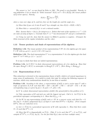
![dimensional representation of U is a direct sum of irreducible representations.
As another example consider the representation theory of quivers.
A quiver is a finite oriented graph Q. A representation of Q over a field k is an assignment
of a k-vector space Vi to every vertex i of Q, and of a linear operator Ah : Vi → Vj to every directed
edge h going from i to j (loops and multiple edges are allowed). We will show that a representation
of a quiver Q is the same thing as a representation of a certain algebra PQ called the path algebra
of Q. Thus one may ask: what are the indecomposable finite dimensional representations of Q?
More specifically, let us say that Q is of finite type if it has finitely many indecomposable
representations.
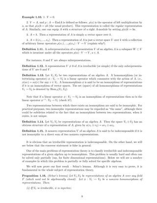
We will prove the following striking theorem, proved by P. Gabriel about 35 years ago:
Theorem 1.2. The finite type property of Q does not depend on the orientation of edges. The
connected graphs that yield quivers of finite type are given by the following list:
• An : ◦−−◦ · · · ◦−−◦
• Dn:
◦−−◦ · · · ◦−−◦
|
◦
• E6 : ◦−−◦−−◦−−◦−−◦
|◦
• E7 : ◦−−◦−−◦−−◦−−◦−−◦
|
◦
• E8 :
◦−−◦−−◦−−◦−−◦−−◦−−◦|
◦
The graphs listed in the theorem are called (simply laced) Dynkin diagrams. These graphs
arise in a multitude of classification problems in mathematics, such as classification of simple Lie
algebras, singularities, platonic solids, reflection groups, etc. In fact, if we needed to make contact
with an alien civilization and show them how sophisticated our civilization is, perhaps showing
them Dynkin diagrams would be the best choice!
As a final example consider the representation theory of finite groups, which is one of the most
fascinating chapters of representation theory. In this theory, one considers representations of the
group algebra A = C[G] of a finite group G – the algebra with basis ag, g ∈ G and multiplication
law agah = agh. We will show that any finite dimensional representation of A is a direct sum of
irreducible representations, i.e., the notions of an irreducible and indecomposable representation
are the same for A (Maschke’s theorem). Another striking result discussed below is the Frobenius
divisibility theorem: the dimension of any irreducible representation of A divides the order of G.
Finally, we will show how to use representation theory of finite groups to prove Burnside’s theorem:
any finite group of order paqb, where p, q are primes, is solvable. Note that this theorem does not
mention representations, which are used only in its proof; a purely group-theoretical proof of this
theorem (not using representations) exists but is much more difficult!
6](https://image.slidesharecdn.com/replect-150306080251-conversion-gate01/85/Replect-6-320.jpg)
![1.2 Algebras
Let us now begin a systematic discussion of representation theory.
Let k be a field. Unless stated otherwise, we will always assume that k is algebraically closed,
i.e., any nonconstant polynomial with coefficients in k has a root in k. The main example is the
field of complex numbers C, but we will also consider fields of characteristic p, such as the algebraic
closure Fp of the finite field Fp of p elements.
Definition 1.3. An associative algebra over k is a vector space A over k together with a bilinear
map A × A → A, (a, b) → ab, such that (ab)c = a(bc).
Definition 1.4. A unit in an associative algebra A is an element 1 ∈ A such that 1a = a1 = a.
Proposition 1.5. If a unit exists, it is unique.
Proof. Let 1, 1′ be two units. Then 1 = 11′ = 1′.
From now on, by an algebra A we will mean an associative algebra with a unit. We will also
assume that A = 0.
Example 1.6. Here are some examples of algebras over k:
1. A = k.
2. A = k[x1, ..., xn] – the algebra of polynomials in variables x1, ..., xn.
3. A = EndV – the algebra of endomorphisms of a vector space V over k (i.e., linear maps, or
operators, from V to itself). The multiplication is given by composition of operators.
4. The free algebra A = k x1, ..., xn . A basis of this algebra consists of words in letters
x1, ..., xn, and multiplication in this basis is simply concatenation of words.
5. The group algebra A = k[G] of a group G. Its basis is {ag, g ∈ G}, with multiplication law
agah = agh.
Definition 1.7. An algebra A is commutative if ab = ba for all a, b ∈ A.
For instance, in the above examples, A is commutative in cases 1 and 2, but not commutative in
cases 3 (if dim V > 1), and 4 (if n > 1). In case 5, A is commutative if and only if G is commutative.
Definition 1.8. A homomorphism of algebras f : A → B is a linear map such that f(xy) =
f(x)f(y) for all x, y ∈ A, and f(1) = 1.
1.3 Representations
Definition 1.9. A representation of an algebra A (also called a left A-module) is a vector space
V together with a homomorphism of algebras ρ : A → EndV .
Similarly, a right A-module is a space V equipped with an antihomomorphism ρ : A → EndV ;
i.e., ρ satisfies ρ(ab) = ρ(b)ρ(a) and ρ(1) = 1.
The usual abbreviated notation for ρ(a)v is av for a left module and va for the right module.
Then the property that ρ is an (anti)homomorphism can be written as a kind of associativity law:
(ab)v = a(bv) for left modules, and (va)b = v(ab) for right modules.
Here are some examples of representations.
7](https://image.slidesharecdn.com/replect-150306080251-conversion-gate01/85/Replect-7-320.jpg)
![(ii) If V2 is irreducible, φ is surjective.
Thus, if both V1 and V2 are irreducible, φ is an isomorphism.
Proof. (i) The kernel K of φ is a subrepresentation of V1. Since φ = 0, this subrepresentation
cannot be V1. So by irreducibility of V1 we have K = 0.
(ii) The image I of φ is a subrepresentation of V2. Since φ = 0, this subrepresentation cannot
be 0. So by irreducibility of V2 we have I = V2.
Corollary 1.17. (Schur’s lemma for algebraically closed fields) Let V be a finite dimensional
irreducible representation of an algebra A over an algebraically closed field k, and φ : V → V is an
intertwining operator. Then φ = λ · Id for some λ ∈ k (a scalar operator).
Remark. Note that this Corollary is false over the field of real numbers: it suffices to take
A = C (regarded as an R-algebra), and V = A.
Proof. Let λ be an eigenvalue of φ (a root of the characteristic polynomial of φ). It exists since k is
an algebraically closed field. Then the operator φ − λId is an intertwining operator V → V , which
is not an isomorphism (since its determinant is zero). Thus by Proposition 1.16 this operator is
zero, hence the result.
Corollary 1.18. Let A be a commutative algebra. Then every irreducible finite dimensional rep-
resentation V of A is 1-dimensional.
Remark. Note that a 1-dimensional representation of any algebra is automatically irreducible.
Proof. Let V be irreducible. For any element a ∈ A, the operator ρ(a) : V → V is an intertwining
operator. Indeed,
ρ(a)ρ(b)v = ρ(ab)v = ρ(ba)v = ρ(b)ρ(a)v
(the second equality is true since the algebra is commutative). Thus, by Schur’s lemma, ρ(a) is
a scalar operator for any a ∈ A. Hence every subspace of V is a subrepresentation. But V is
irreducible, so 0 and V are the only subspaces of V . This means that dim V = 1 (since V = 0).
Example 1.19. 1. A = k. Since representations of A are simply vector spaces, V = A is the only
irreducible and the only indecomposable representation.
2. A = k[x]. Since this algebra is commutative, the irreducible representations of A are its
1-dimensional representations. As we discussed above, they are defined by a single operator ρ(x).
In the 1-dimensional case, this is just a number from k. So all the irreducible representations of A
are Vλ = k, λ ∈ k, in which the action of A defined by ρ(x) = λ. Clearly, these representations are
pairwise non-isomorphic.
The classification of indecomposable representations of k[x] is more interesting. To obtain it,
recall that any linear operator on a finite dimensional vector space V can be brought to Jordan
normal form. More specifically, recall that the Jordan block Jλ,n is the operator on kn which in
the standard basis is given by the formulas Jλ,nei = λei + ei−1 for i > 1, and Jλ,ne1 = λe1. Then
for any linear operator B : V → V there exists a basis of V such that the matrix of B in this basis
is a direct sum of Jordan blocks. This implies that all the indecomposable representations of A are
Vλ,n = kn, λ ∈ k, with ρ(x) = Jλ,n. The fact that these representations are indecomposable and
pairwise non-isomorphic follows from the Jordan normal form theorem (which in particular says
that the Jordan normal form of an operator is unique up to permutation of blocks).
9](https://image.slidesharecdn.com/replect-150306080251-conversion-gate01/85/Replect-9-320.jpg)
![This example shows that an indecomposable representation of an algebra need not be irreducible.
3. The group algebra A = k[G], where G is a group. A representation of A is the same thing as
a representation of G, i.e., a vector space V together with a group homomorphism ρ : G → Aut(V ),
whre Aut(V ) = GL(V ) denotes the group of invertible linear maps from the space V to itself.
Problem 1.20. Let V be a nonzero finite dimensional representation of an algebra A. Show that
it has an irreducible subrepresentation. Then show by example that this does not always hold for
infinite dimensional representations.
Problem 1.21. Let A be an algebra over a field k. The center Z(A) of A is the set of all elements
z ∈ A which commute with all elements of A. For example, if A is commutative then Z(A) = A.
(a) Show that if V is an irreducible finite dimensional representation of A then any element
z ∈ Z(A) acts in V by multiplication by some scalar χV (z). Show that χV : Z(A) → k is a
homomorphism. It is called the central character of V .
(b) Show that if V is an indecomposable finite dimensional representation of A then for any
z ∈ Z(A), the operator ρ(z) by which z acts in V has only one eigenvalue χV (z), equal to the
scalar by which z acts on some irreducible subrepresentation of V . Thus χV : Z(A) → k is a
homomorphism, which is again called the central character of V .
(c) Does ρ(z) in (b) have to be a scalar operator?
Problem 1.22. Let A be an associative algebra, and V a representation of A. By EndA(V ) one
denotes the algebra of all homomorphisms of representations V → V . Show that EndA(A) = Aop,
the algebra A with opposite multiplication.
Problem 1.23. Prove the following “Infinite dimensional Schur’s lemma” (due to Dixmier): Let
A be an algebra over C and V be an irreducible representation of A with at most countable basis.
Then any homomorphism of representations φ : V → V is a scalar operator.
Hint. By the usual Schur’s lemma, the algebra D := EndA(V ) is an algebra with division.
Show that D is at most countably dimensional. Suppose φ is not a scalar, and consider the subfield
C(φ) ⊂ D. Show that C(φ) is a transcendental extension of C. Derive from this that C(φ) is
uncountably dimensional and obtain a contradiction.
1.4 Ideals
A left ideal of an algebra A is a subspace I ⊆ A such that aI ⊆ I for all a ∈ A. Similarly, a right
ideal of an algebra A is a subspace I ⊆ A such that Ia ⊆ I for all a ∈ A. A two-sided ideal is a
subspace that is both a left and a right ideal.
Left ideals are the same as subrepresentations of the regular representation A. Right ideals are
the same as subrepresentations of the regular representation of the opposite algebra Aop.
Below are some examples of ideals:
• If A is any algebra, 0 and A are two-sided ideals. An algebra A is called simple if 0 and A
are its only two-sided ideals.
• If φ : A → B is a homomorphism of algebras, then ker φ is a two-sided ideal of A.
• If S is any subset of an algebra A, then the two-sided ideal generated by S is denoted S and
is the span of elements of the form asb, where a, b ∈ A and s ∈ S. Similarly we can define
S ℓ = span{as} and S r = span{sb}, the left, respectively right, ideal generated by S.
10](https://image.slidesharecdn.com/replect-150306080251-conversion-gate01/85/Replect-10-320.jpg)
![1.5 Quotients
Let A be an algebra and I a two-sided ideal in A. Then A/I is the set of (additive) cosets of I.
Let π : A → A/I be the quotient map. We can define multiplication in A/I by π(a) · π(b) := π(ab).
This is well defined because if π(a) = π(a′) then
π(a′
b) = π(ab + (a′
− a)b) = π(ab) + π((a′
− a)b) = π(ab)
because (a′ − a)b ∈ Ib ⊆ I = ker π, as I is a right ideal; similarly, if π(b) = π(b′) then
π(ab′
) = π(ab + a(b′
− b)) = π(ab) + π(a(b′
− b)) = π(ab)
because a(b′ − b) ∈ aI ⊆ I = ker π, as I is also a left ideal. Thus, A/I is an algebra.
Similarly, if V is a representation of A, and W ⊂ V is a subrepresentation, then V/W is also a
representation. Indeed, let π : V → V/W be the quotient map, and set ρV/W (a)π(x) := π(ρV (a)x).
Above we noted that left ideals of A are subrepresentations of the regular representation of A,
and vice versa. Thus, if I is a left ideal in A, then A/I is a representation of A.
Problem 1.24. Let A = k[x1, ..., xn] and I = A be any ideal in A containing all homogeneous
polynomials of degree ≥ N. Show that A/I is an indecomposable representation of A.
Problem 1.25. Let V = 0 be a representation of A. We say that a vector v ∈ V is cyclic if it
generates V , i.e., Av = V . A representation admitting a cyclic vector is said to be cyclic. Show
that
(a) V is irreducible if and only if all nonzero vectors of V are cyclic.
(b) V is cyclic if and only if it is isomorphic to A/I, where I is a left ideal in A.
(c) Give an example of an indecomposable representation which is not cyclic.
Hint. Let A = C[x, y]/I2, where I2 is the ideal spanned by homogeneous polynomials of degree
≥ 2 (so A has a basis 1, x, y). Let V = A∗ be the space of linear functionals on A, with the action
of A given by (ρ(a)f)(b) = f(ba). Show that V provides such an example.
1.6 Algebras defined by generators and relations
If f1, . . . , fm are elements of the free algebra k x1, . . . , xn , we say that the algebra
A := k x1, . . . , xn / {f1, . . . , fm} is generated by x1, . . . , xn with defining relations f1 = 0, . . . , fm =
0.
1.7 Examples of algebras
1. The Weyl algebra, k x, y / yx − xy − 1 .
2. The q-Weyl algebra, generated by x, x−1, y, y−1 with defining relations yx = qxy and xx−1 =
x−1x = yy−1 = y−1y = 1.
Proposition. (i) A basis for the Weyl algebra A is {xiyj, i, j ≥ 0}.
(ii) A basis for the q-Weyl algebra Aq is {xiyj, i, j ∈ Z}.
11](https://image.slidesharecdn.com/replect-150306080251-conversion-gate01/85/Replect-11-320.jpg)
![Proof. (i) First let us show that the elements xiyj are a spanning set for A. To do this, note that
any word in x, y can be ordered to have all the x on the left of the y, at the cost of interchanging
some x and y. Since yx − xy = 1, this will lead to error terms, but these terms will be sums of
monomials that have a smaller number of letters x, y than the original word. Therefore, continuing
this process, we can order everything and represent any word as a linear combination of xiyj.
The proof that xiyj are linearly independent is based on representation theory. Namely, let a be
a variable, and E = tak[a][t, t−1] (here ta is just a formal symbol, so really E = k[a][t, t−1]). Then E
is a representation of A with action given by xf = tf and yf = df
dt (where d(ta+n)
dt := (a+n)ta+n−1).
Suppose now that we have a nontrivial linear relation cijxiyj = 0. Then the operator
L = cijti d
dt
j
acts by zero in E. Let us write L as
L =
r
j=0
Qj(t)
d
dt
j
,
where Qr = 0. Then we have
Lta
=
r
j=0
Qj(t)a(a − 1)...(a − j + 1)ta−j
.
This must be zero, so we have r
j=0 Qj(t)a(a − 1)...(a − j + 1)t−j = 0 in k[a][t, t−1]. Taking the
leading term in a, we get Qr(t) = 0, a contradiction.
(ii) Any word in x, y, x−1, y−1 can be ordered at the cost of multiplying it by a power of q. This
easily implies both the spanning property and the linear independence.
Remark. The proof of (i) shows that the Weyl algebra A can be viewed as the algebra of
polynomial differential operators in one variable t.
The proof of (i) also brings up the notion of a faithful representation.
Definition. A representation ρ : A → End V is faithful if ρ is injective.
For example, k[t] is a faithful representation of the Weyl algebra, if k has characteristic zero
(check it!), but not in characteristic p, where (d/dt)pQ = 0 for any polynomial Q. However, the
representation E = tak[a][t, t−1], as we’ve seen, is faithful in any characteristic.
Problem 1.26. Let A be the Weyl algebra, generated by two elements x, y with the relation
yx − xy − 1 = 0.
(a) If chark = 0, what are the finite dimensional representations of A? What are the two-sided
ideals in A?
Hint. For the first question, use the fact that for two square matrices B, C, Tr(BC) = Tr(CB).
For the second question, show that any nonzero two-sided ideal in A contains a nonzero polynomial
in x, and use this to characterize this ideal.
Suppose for the rest of the problem that chark = p.
(b) What is the center of A?
12](https://image.slidesharecdn.com/replect-150306080251-conversion-gate01/85/Replect-12-320.jpg)
![1. p2
i = pi, pipj = 0 for i = j
2. ahph′ = ah, ahpj = 0 for j = h′
3. ph′′ ah = ah, piah = 0 for i = h′′
We now justify our statement that a representation of a quiver is the same thing as a represen-
tation of the path algebra of a quiver.
Let V be a representation of the path algebra PQ. From this representation, we can construct a
representation of Q as follows: let Vi = piV, and for any edge h, let xh = ah|ph′ V : ph′ V −→ ph′′ V
be the operator corresponding to the one-edge path h.
Similarly, let (Vi, xh) be a representation of a quiver Q. From this representation, we can
construct a representation of the path algebra PQ: let V = i Vi, let pi : V → Vi → V be the
projection onto Vi, and for any path p = h1...hm let ap = xh1 ...xhm : Vh′
m
→ Vh′′
1
be the composition
of the operators corresponding to the edges occurring in p (and the action of this operator on the
other Vi is zero).
It is clear that the above assignments V → (piV) and (Vi) → i Vi are inverses of each other.
Thus, we have a bijection between isomorphism classes of representations of the algebra PQ and of
the quiver Q.
Remark 1.34. In practice, it is generally easier to consider a representation of a quiver as in
Definition 1.30.
We lastly define several previous concepts in the context of quivers representations.
Definition 1.35. A subrepresentation of a representation (Vi, xh) of a quiver Q is a representation
(Wi, x′
h) where Wi ⊆ Vi for all i ∈ I and where xh(Wh′ ) ⊆ Wh′′ and x′
h = xh|Wh′ : Wh′ −→ Wh′′ for
all h ∈ E.
Definition 1.36. The direct sum of two representations (Vi, xh) and (Wi, yh) is the representation
(Vi ⊕ Wi, xh ⊕ yh).
As with representations of algebras, a nonzero representation (Vi) of a quiver Q is said to be
irreducible if its only subrepresentations are (0) and (Vi) itself, and indecomposable if it is not
isomorphic to a direct sum of two nonzero representations.
Definition 1.37. Let (Vi, xh) and (Wi, yh) be representations of the quiver Q. A homomorphism
ϕ : (Vi) −→ (Wi) of quiver representations is a collection of maps ϕi : Vi −→ Wi such that
yh ◦ ϕh′ = ϕh′′ ◦ xh for all h ∈ E.
Problem 1.38. Let A be a Z+-graded algebra, i.e., A = ⊕n≥0A[n], and A[n] · A[m] ⊂ A[n + m].
If A[n] is finite dimensional, it is useful to consider the Hilbert series hA(t) = dim A[n]tn (the
generating function of dimensions of A[n]). Often this series converges to a rational function, and
the answer is written in the form of such function. For example, if A = k[x] and deg(xn) = n then
hA(t) = 1 + t + t2
+ ... + tn
+ ... =
1
1 − t
Find the Hilbert series of:
(a) A = k[x1, ..., xm] (where the grading is by degree of polynomials);
14](https://image.slidesharecdn.com/replect-150306080251-conversion-gate01/85/Replect-14-320.jpg)
![(b) A = k < x1, ..., xm > (the grading is by length of words);
(c) A is the exterior (=Grassmann) algebra ∧k[x1, ..., xm], generated over some field k by
x1, ..., xm with the defining relations xixj + xjxi = 0 and x2
i = 0 for all i, j (the grading is by
degree).
(d) A is the path algebra PQ of a quiver Q (the grading is defined by deg(pi) = 0, deg(ah) = 1).
Hint. The closed answer is written in terms of the adjacency matrix MQ of Q.
1.9 Lie algebras
Let g be a vector space over a field k, and let [ , ] : g × g −→ g be a skew-symmetric bilinear map.
(That is, [a, a] = 0, and hence [a, b] = −[b, a]).
Definition 1.39. (g, [ , ]) is a Lie algebra if [ , ] satisfies the Jacobi identity
[a, b] , c + [b, c] , a + [c, a] , b = 0. (2)
Example 1.40. Some examples of Lie algebras are:
1. Any space g with [ , ] = 0 (abelian Lie algebra).
2. Any associative algebra A with [a, b] = ab − ba .
3. Any subspace U of an associative algebra A such that [a, b] ∈ U for all a, b ∈ U.
4. The space Der(A) of derivations of an algebra A, i.e. linear maps D : A → A which satisfy
the Leibniz rule:
D(ab) = D(a)b + aD(b).
Remark 1.41. Derivations are important because they are the “infinitesimal version” of automor-
phisms (i.e., isomorphisms onto itself). For example, assume that g(t) is a differentiable family of
automorphisms of a finite dimensional algebra A over R or C parametrized by t ∈ (−ǫ, ǫ) such that
g(0) = Id. Then D := g′(0) : A → A is a derivation (check it!). Conversely, if D : A → A is a
derivation, then etD is a 1-parameter family of automorphisms (give a proof!).
This provides a motivation for the notion of a Lie algebra. Namely, we see that Lie algebras
arise as spaces of infinitesimal automorphisms (=derivations) of associative algebras. In fact, they
similarly arise as spaces of derivations of any kind of linear algebraic structures, such as Lie algebras,
Hopf algebras, etc., and for this reason play a very important role in algebra.
Here are a few more concrete examples of Lie algebras:
1. R3 with [u, v] = u × v, the cross-product of u and v.
2. sl(n), the set of n × n matrices with trace 0.
For example, sl(2) has the basis
e =
0 1
0 0
f =
0 0
1 0
h =
1 0
0 −1
with relations
[h, e] = 2e, [h, f] = −2f, [e, f] = h.
15](https://image.slidesharecdn.com/replect-150306080251-conversion-gate01/85/Replect-15-320.jpg)
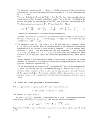
![3. The Heisenberg Lie algebra H of matrices
0 ∗ ∗
0 0 ∗
0 0 0
It has the basis
x =
0 0 0
0 0 1
0 0 0
y =
0 1 0
0 0 0
0 0 0
c =
0 0 1
0 0 0
0 0 0
with relations [y, x] = c and [y, c] = [x, c] = 0.
4. The algebra aff(1) of matrices ( ∗ ∗
0 0 )
Its basis consists of X = ( 1 0
0 0 ) and Y = ( 0 1
0 0 ), with [X, Y ] = Y .
5. so(n), the space of skew-symmetric n × n matrices, with [a, b] = ab − ba.
Exercise. Show that Example 1 is a special case of Example 5 (for n = 3).
Definition 1.42. Let g1, g2 be Lie algebras. A homomorphism ϕ : g1 −→ g2 of Lie algebras is a
linear map such that ϕ([a, b]) = [ϕ(a), ϕ(b)].
Definition 1.43. A representation of a Lie algebra g is a vector space V with a homomorphism
of Lie algebras ρ : g −→ End V .
Example 1.44. Some examples of representations of Lie algebras are:
1. V = 0.
2. Any vector space V with ρ = 0 (the trivial representation).
3. The adjoint representation V = g with ρ(a)(b) := [a, b]. That this is a representation follows
from Equation (2). Thus, the meaning of the Jacobi identity is that it is equivalent to the
existence of the adjoint representation.
It turns out that a representation of a Lie algebra g is the same thing as a representation of a
certain associative algebra U(g). Thus, as with quivers, we can view the theory of representations
of Lie algebras as a part of the theory of representations of associative algebras.
Definition 1.45. Let g be a Lie algebra with basis xi and [ , ] defined by [xi, xj] = k ck
ijxk. The
universal enveloping algebra U(g) is the associative algebra generated by the xi’s with the
defining relations xixj − xjxi = k ck
ijxk.
Remark. This is not a very good definition since it depends on the choice of a basis. Later we
will give an equivalent definition which will be basis-independent.
Exercise. Explain why a representation of a Lie algebra is the same thing as a representation
of its universal enveloping algebra.
Example 1.46. The associative algebra U(sl(2)) is the algebra generated by e, f, h with relations
he − eh = 2e hf − fh = −2f ef − fe = h.
Example 1.47. The algebra U(H), where H is the Heisenberg Lie algebra, is the algebra generated
by x, y, c with the relations
yx − xy = c yc − cy = 0 xc − cx = 0.
Note that the Weyl algebra is the quotient of U(H) by the relation c = 1.
16](https://image.slidesharecdn.com/replect-150306080251-conversion-gate01/85/Replect-16-320.jpg)
![Similarly, if C is another k-algebra, and if the left B-module structure on W is part of a (B, C)-
bimodule structure, then V ⊗B W becomes a right C-module by (v ⊗B w) c = v ⊗B wc for any
c ∈ C, v ∈ V and w ∈ W.
If V is an (A, B)-bimodule and W is a (B, C)-bimodule, then these two structures on V ⊗B W
can be combined into one (A, C)-bimodule structure on V ⊗B W.
(a) Let A, B, C, D be four algebras. Let V be an (A, B)-bimodule, W be a (B, C)-bimodule,
and X a (C, D)-bimodule. Prove that (V ⊗B W) ⊗C X ∼= V ⊗B (W ⊗C X) as (A, D)-bimodules.
The isomorphism (from left to right) is given by (v ⊗B w) ⊗C x → v ⊗B (w ⊗C x) for all v ∈ V ,
w ∈ W and x ∈ X.
(b) If A, B, C are three algebras, and if V is an (A, B)-bimodule and W an (A, C)-bimodule,
then the vector space HomA (V, W) (the space of all left A-linear homomorphisms from V to W)
canonically becomes a (B, C)-bimodule by setting (bf) (v) = f (vb) for all b ∈ B, f ∈ HomA (V, W)
and v ∈ V and (fc) (v) = f (v) c for all c ∈ C, f ∈ HomA (V, W) and v ∈ V .
Let A, B, C, D be four algebras. Let V be a (B, A)-bimodule, W be a (C, B)-bimodule, and X a
(C, D)-bimodule. Prove that HomB (V, HomC (W, X)) ∼= HomC (W ⊗B V, X) as (A, D)-bimodules.
The isomorphism (from left to right) is given by f → (w ⊗B v → f (v) w) for all v ∈ V , w ∈ W
and f ∈ HomB (V, HomC (W, X)).
1.11 The tensor algebra
The notion of tensor product allows us to give more conceptual (i.e., coordinate free) definitions
of the free algebra, polynomial algebra, exterior algebra, and universal enveloping algebra of a Lie
algebra.
Namely, given a vector space V , define its tensor algebra TV over a field k to be TV = ⊕n≥0V ⊗n,
with multiplication defined by a · b := a ⊗ b, a ∈ V ⊗n, b ∈ V ⊗m. Observe that a choice of a basis
x1, ..., xN in V defines an isomorphism of TV with the free algebra k < x1, ..., xn >.
Also, one can make the following definition.
Definition 1.50. (i) The symmetric algebra SV of V is the quotient of TV by the ideal generated
by v ⊗ w − w ⊗ v, v, w ∈ V .
(ii) The exterior algebra ∧V of V is the quotient of TV by the ideal generated by v ⊗ v, v ∈ V .
(iii) If V is a Lie algebra, the universal enveloping algebra U(V ) of V is the quotient of TV by
the ideal generated by v ⊗ w − w ⊗ v − [v, w], v, w ∈ V .
It is easy to see that a choice of a basis x1, ..., xN in V identifies SV with the polynomial algebra
k[x1, ..., xN ], ∧V with the exterior algebra ∧k(x1, ..., xN ), and the universal enveloping algebra U(V )
with one defined previously.
Also, it is easy to see that we have decompositions SV = ⊕n≥0SnV , ∧V = ⊕n≥0 ∧n V .
1.12 Hilbert’s third problem
Problem 1.51. It is known that if A and B are two polygons of the same area then A can be cut
by finitely many straight cuts into pieces from which one can make B. David Hilbert asked in 1900
whether it is true for polyhedra in 3 dimensions. In particular, is it true for a cube and a regular
tetrahedron of the same volume?
19](https://image.slidesharecdn.com/replect-150306080251-conversion-gate01/85/Replect-19-320.jpg)
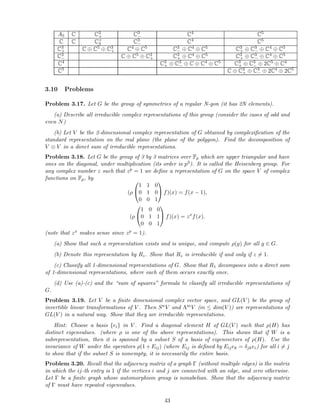
![(e) Let Nv be the smallest N satisfying (c). Show that λ = Nv − 1.
(f) Show that for each N > 0, there exists a unique up to isomorphism irreducible representation
of sl(2) of dimension N. Compute the matrices E, F, H in this representation using a convenient
basis. (For V finite dimensional irreducible take λ as in (a) and v ∈ V (λ) an eigenvector of H.
Show that v, Fv, ..., Fλv is a basis of V , and compute the matrices of the operators E, F, H in this
basis.)
Denote the λ + 1-dimensional irreducible representation from (f) by Vλ. Below you will show
that any finite dimensional representation is a direct sum of Vλ.
(g) Show that the operator C = EF + FE + H2/2 (the so-called Casimir operator) commutes
with E, F, H and equals λ(λ+2)
2 Id on Vλ.
Now it will be easy to prove the direct sum decomposition. Namely, assume the contrary, and
let V be a reducible representation of the smallest dimension, which is not a direct sum of smaller
representations.
(h) Show that C has only one eigenvalue on V , namely λ(λ+2)
2 for some nonnegative integer λ.
(use that the generalized eigenspace decomposition of C must be a decomposition of representations).
(i) Show that V has a subrepresentation W = Vλ such that V/W = nVλ for some n (use (h)
and the fact that V is the smallest which cannot be decomposed).
(j) Deduce from (i) that the eigenspace V (λ) of H is n + 1-dimensional. If v1, ..., vn+1 is its
basis, show that Fjvi, 1 ≤ i ≤ n + 1, 0 ≤ j ≤ λ are linearly independent and therefore form a basis
of V (establish that if Fx = 0 and Hx = µx then Cx = µ(µ−2)
2 x and hence µ = −λ).
(k) Define Wi = span(vi, Fvi, ..., Fλvi). Show that Vi are subrepresentations of V and derive a
contradiction with the fact that V cannot be decomposed.
(l) (Jacobson-Morozov Lemma) Let V be a finite dimensional complex vector space and A : V →
V a nilpotent operator. Show that there exists a unique, up to an isomorphism, representation of
sl(2) on V such that E = A. (Use the classification of the representations and the Jordan normal
form theorem)
(m) (Clebsch-Gordan decomposition) Find the decomposition into irreducibles of the represen-
tation Vλ ⊗ Vµ of sl(2).
Hint. For a finite dimensional representation V of sl(2) it is useful to introduce the character
χV (x) = Tr(exH), x ∈ C. Show that χV ⊕W (x) = χV (x) + χW (x) and χV ⊗W (x) = χV (x)χW (x).
Then compute the character of Vλ and of Vλ ⊗Vµ and derive the decomposition. This decomposition
is of fundamental importance in quantum mechanics.
(n) Let V = CM ⊗ CN , and A = JM (0) ⊗ IdN + IdM ⊗ JN (0), where Jn(0) is the Jordan block
of size n with eigenvalue zero (i.e., Jn(0)ei = ei−1, i = 2, ..., n, and Jn(0)e1 = 0). Find the Jordan
normal form of A using (l),(m).
1.15 Problems on Lie algebras
Problem 1.56. (Lie’s Theorem) The commutant K(g) of a Lie algebra g is the linear span
of elements [x, y], x, y ∈ g. This is an ideal in g (i.e., it is a subrepresentation of the adjoint
representation). A finite dimensional Lie algebra g over a field k is said to be solvable if there
exists n such that Kn(g) = 0. Prove the Lie theorem: if k = C and V is a finite dimensional
irreducible representation of a solvable Lie algebra g then V is 1-dimensional.
21](https://image.slidesharecdn.com/replect-150306080251-conversion-gate01/85/Replect-21-320.jpg)
![Hint. Prove the result by induction in dimension. By the induction assumption, K(g) has a
common eigenvector v in V , that is there is a linear function χ : K(g) → C such that av = χ(a)v
for any a ∈ K(g). Show that g preserves common eigenspaces of K(g) (for this you will need to
show that χ([x, a]) = 0 for x ∈ g and a ∈ K(g). To prove this, consider the smallest vector subspace
U containing v and invariant under x. This subspace is invariant under K(g) and any a ∈ K(g)
acts with trace dim(U)χ(a) in this subspace. In particular 0 = Tr([x, a]) = dim(U)χ([x, a]).).
Problem 1.57. Classify irreducible finite dimensional representations of the two dimensional Lie
algebra with basis X, Y and commutation relation [X, Y ] = Y . Consider the cases of zero and
positive characteristic. Is the Lie theorem true in positive characteristic?
Problem 1.58. (hard!) For any element x of a Lie algebra g let ad(x) denote the operator g →
g, y → [x, y]. Consider the Lie algebra gn generated by two elements x, y with the defining relations
ad(x)2(y) = ad(y)n+1(x) = 0.
(a) Show that the Lie algebras g1, g2, g3 are finite dimensional and find their dimensions.
(b) (harder!) Show that the Lie algebra g4 has infinite dimension. Construct explicitly a basis
of this algebra.
22](https://image.slidesharecdn.com/replect-150306080251-conversion-gate01/85/Replect-22-320.jpg)
![Example 2.14. 1. Let A = k[x]/(xn). This algebra has a unique irreducible representation, which
is a 1-dimensional space k, in which x acts by zero. So the radical Rad(A) is the ideal (x).
2. Let A be the algebra of upper triangular n by n matrices. It is easy to check that the
irreducible representations of A are Vi, i = 1, ..., n, which are 1-dimensional, and any matrix x acts
by xii. So the radical Rad(A) is the ideal of strictly upper triangular matrices (as it is a nilpotent
ideal and contains the radical). A similar result holds for block-triangular matrices.
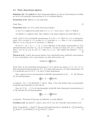
Definition 2.15. A finite dimensional algebra A is said to be semisimple if Rad(A) = 0.
Proposition 2.16. For a finite dimensional algebra A, the following are equivalent:
1. A is semisimple.
2. i (dim Vi)2
= dim A, where the Vi’s are the irreducible representations of A.
3. A ∼= i Matdi
(k) for some di.
4. Any finite dimensional representation of A is completely reducible (that is, isomorphic to a
direct sum of irreducible representations).
5. A is a completely reducible representation of A.
Proof. As dim A−dim Rad(A) = i (dim Vi)2
, clearly dim A = i (dim Vi)2
if and only if Rad(A) =
0. Thus, (1) ⇔ (2).
Next, by Theorem 2.12, if Rad(A) = 0, then clearly A ∼= i Matdi
(k) for di = dim Vi. Thus,
(1) ⇒ (3). Conversely, if A ∼= i Matdi
(k), then by Theorem 2.6, Rad(A) = 0, so A is semisimple.
Thus (3) ⇒ (1).
Next, (3) ⇒ (4) by Theorem 2.6. Clearly (4) ⇒ (5). To see that (5) ⇒ (3), let A = i niVi.
Consider EndA(A) (endomorphisms of A as a representation of A). As the Vi’s are pairwise non-
isomorphic, by Schur’s lemma, no copy of Vi in A can be mapped to a distinct Vj. Also, again by
Schur’s lemma, EndA (Vi) = k. Thus, EndA(A) ∼= i Matni (k). But EndA(A) ∼= Aop by Problem
1.22, so Aop ∼= i Matni (k). Thus, A ∼= ( i Matni (k))op
= i Matni (k), as desired.
2.6 Characters of representations
Let A be an algebra and V a finite-dimensional representation of A with action ρ. Then the
character of V is the linear function χV : A → k given by
χV (a) = tr|V (ρ(a)).
If [A, A] is the span of commutators [x, y] := xy − yx over all x, y ∈ A, then [A, A] ⊆ ker χV . Thus,
we may view the character as a mapping χV : A/[A, A] → k.
Exercise. Show that if W ⊂ V are finite dimensional representations of A, then χV = χW +
χV/W .
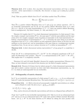
Theorem 2.17. (i) Characters of (distinct) irreducible finite-dimensional representations of A are
linearly independent.
(ii) If A is a finite-dimensional semisimple algebra, then these characters form a basis of
(A/[A, A])∗.
27](https://image.slidesharecdn.com/replect-150306080251-conversion-gate01/85/Replect-27-320.jpg)
![Proof. (i) If V1, . . . , Vr are nonisomorphic irreducible finite-dimensional representations of A, then
ρV1 ⊕· · ·⊕ρVr : A → End V1 ⊕· · ·⊕End Vr is surjective by the density theorem, so χV1 , . . . , χVr are
linearly independent. (Indeed, if λiχVi (a) = 0 for all a ∈ A, then λiTr(Mi) = 0 for all Mi ∈
EndkVi. But each tr(Mi) can range independently over k, so it must be that λ1 = · · · = λr = 0.)
(ii) First we prove that [Matd(k), Matd(k)] = sld(k), the set of all matrices with trace 0. It is
clear that [Matd(k), Matd(k)] ⊆ sld(k). If we denote by Eij the matrix with 1 in the ith row of the
jth column and 0’s everywhere else, we have [Eij, Ejm] = Eim for i = m, and [Ei,i+1, Ei+1,i] = Eii −
Ei+1,i+1. Now {Eim}∪{Eii−Ei+1,i+1} forms a basis in sld(k), so indeed [Matd(k), Matd(k)] = sld(k),
as claimed.
By semisimplicity, we can write A = Matd1 (k) ⊕ · · · ⊕ Matdr (k). Then [A, A] = sld1 (k) ⊕ · · · ⊕
sldr (k), and A/[A, A] ∼= kr. By Theorem 2.6, there are exactly r irreducible representations of A
(isomorphic to kd1 , . . . , kdr
, respectively), and therefore r linearly independent characters on the
r-dimensional vector space A/[A, A]. Thus, the characters form a basis.
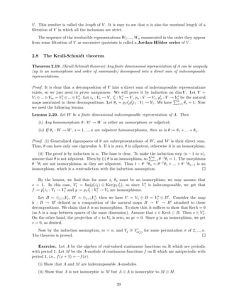
2.7 The Jordan-H¨older theorem
We will now state and prove two important theorems about representations of finite dimensional
algebras - the Jordan-H¨older theorem and the Krull-Schmidt theorem.
Theorem 2.18. (Jordan-H¨older theorem). Let V be a finite dimensional representation of A,
and 0 = V0 ⊂ V1 ⊂ ... ⊂ Vn = V , 0 = V ′
0 ⊂ ... ⊂ V ′
m = V be filtrations of V , such that the
representations Wi := Vi/Vi−1 and W′
i := V ′
i /V ′
i−1 are irreducible for all i. Then n = m, and there
exists a permutation σ of 1, ..., n such that Wσ(i) is isomorphic to W′
i .
Proof. First proof (for k of characteristic zero). The character of V obviously equals the sum
of characters of Wi, and also the sum of characters of W′
i . But by Theorem 2.17, the charac-
ters of irreducible representations are linearly independent, so the multiplicity of every irreducible
representation W of A among Wi and among W′
i are the same. This implies the theorem. 3
Second proof (general). The proof is by induction on dim V . The base of induction is clear,
so let us prove the induction step. If W1 = W′
1 (as subspaces), we are done, since by the induction
assumption the theorem holds for V/W1. So assume W1 = W′
1. In this case W1 ∩ W′
1 = 0 (as
W1, W′
1 are irreducible), so we have an embedding f : W1 ⊕ W′
1 → V . Let U = V/(W1 ⊕ W′
1), and
0 = U0 ⊂ U1 ⊂ ... ⊂ Up = U be a filtration of U with simple quotients Zi = Ui/Ui−1 (it exists by
Lemma 2.8). Then we see that:
1) V/W1 has a filtration with successive quotients W′
1, Z1, ..., Zp, and another filtration with
successive quotients W2, ...., Wn.
2) V/W′
1 has a filtration with successive quotients W1, Z1, ..., Zp, and another filtration with
successive quotients W′
2, ...., W′
n.
By the induction assumption, this means that the collection of irreducible representations with
multiplicities W1, W′
1, Z1, ..., Zp coincides on one hand with W1, ..., Wn, and on the other hand, with
W′
1, ..., W′
m. We are done.
The Jordan-H¨older theorem shows that the number n of terms in a filtration of V with irre-
ducible successive quotients does not depend on the choice of a filtration, and depends only on
3
This proof does not work in characteristic p because it only implies that the multiplicities of Wi and W ′
i are the
same modulo p, which is not sufficient. In fact, the character of the representation pV , where V is any representation,
is zero.
28](https://image.slidesharecdn.com/replect-150306080251-conversion-gate01/85/Replect-28-320.jpg)
![Remark. Thus, we see that in general, the Krull-Schmidt theorem fails for infinite dimensional
modules. However, it still holds for modules of finite length, i.e., modules M such that any filtration
of M has length bounded above by a certain constant l = l(M).
2.9 Problems
Problem 2.21. Extensions of representations. Let A be an algebra, and V, W be a pair of
representations of A. We would like to classify representations U of A such that V is a subrepre-
sentation of U, and U/V = W. Of course, there is an obvious example U = V ⊕ W, but are there
any others?
Suppose we have a representation U as above. As a vector space, it can be (non-uniquely)
identified with V ⊕ W, so that for any a ∈ A the corresponding operator ρU (a) has block triangular
form
ρU (a) =
ρV (a) f(a)
0 ρW (a)
,
where f : A → Homk(W, V ) is a linear map.
(a) What is the necessary and sufficient condition on f(a) under which ρU (a) is a repre-
sentation? Maps f satisfying this condition are called (1-)cocycles (of A with coefficients in
Homk(W, V )). They form a vector space denoted Z1(W, V ).
(b) Let X : W → V be a linear map. The coboundary of X, dX, is defined to be the function A →
Homk(W, V ) given by dX(a) = ρV (a)X−XρW (a). Show that dX is a cocycle, which vanishes if and
only if X is a homomorphism of representations. Thus coboundaries form a subspace B1(W, V ) ⊂
Z1(W, V ), which is isomorphic to Homk(W, V )/HomA(W, V ). The quotient Z1(W, V )/B1(W, V ) is
denoted Ext1
(W, V ).
(c) Show that if f, f′ ∈ Z1(W, V ) and f − f′ ∈ B1(W, V ) then the corresponding extensions
U, U′ are isomorphic representations of A. Conversely, if φ : U → U′ is an isomorphism such that
φ(a) =
1V ∗
0 1W
then f − f′ ∈ B1(V, W). Thus, the space Ext1(W, V ) “classifies” extensions of W by V .
(d) Assume that W, V are finite dimensional irreducible representations of A. For any f ∈
Ext1(W, V ), let Uf be the corresponding extension. Show that Uf is isomorphic to Uf′ as repre-
sentations if and only if f and f′ are proportional. Thus isomorphism classes (as representations)
of nontrivial extensions of W by V (i.e., those not isomorphic to W ⊕ V ) are parametrized by the
projective space PExt1
(W, V ). In particular, every extension is trivial if and only if Ext1
(W, V ) = 0.
Problem 2.22. (a) Let A = C[x1, ..., xn], and Va, Vb be one-dimensional representations in which
xi act by ai and bi, respectively (ai, bi ∈ C). Find Ext1
(Va, Vb) and classify 2-dimensional repre-
sentations of A.
(b) Let B be the algebra over C generated by x1, ..., xn with the defining relations xixj = 0 for
all i, j. Show that for n > 1 the algebra B has infinitely many non-isomorphic indecomposable
representations.
Problem 2.23. Let Q be a quiver without oriented cycles, and PQ the path algebra of Q. Find
irreducible representations of PQ and compute Ext1
between them. Classify 2-dimensional repre-
sentations of PQ.
30](https://image.slidesharecdn.com/replect-150306080251-conversion-gate01/85/Replect-30-320.jpg)
![Problem 2.24. Let A be an algebra, and V a representation of A. Let ρ : A → EndV . A formal
deformation of V is a formal series
˜ρ = ρ0 + tρ1 + ... + tn
ρn + ...,
where ρi : A → End(V ) are linear maps, ρ0 = ρ, and ˜ρ(ab) = ˜ρ(a)˜ρ(b).
If b(t) = 1 + b1t + b2t2 + ..., where bi ∈ End(V ), and ˜ρ is a formal deformation of ρ, then b˜ρb−1
is also a deformation of ρ, which is said to be isomorphic to ˜ρ.
(a) Show that if Ext1
(V, V ) = 0, then any deformation of ρ is trivial, i.e., isomorphic to ρ.
(b) Is the converse to (a) true? (consider the algebra of dual numbers A = k[x]/x2).
Problem 2.25. The Clifford algebra. Let V be a finite dimensional complex vector space
equipped with a symmetric bilinear form (, ). The Clifford algebra Cl(V ) is the quotient of the
tensor algebra TV by the ideal generated by the elements v ⊗ v − (v, v)1, v ∈ V . More explicitly, if
xi, 1 ≤ i ≤ N is a basis of V and (xi, xj) = aij then Cl(V ) is generated by xi with defining relations
xixj + xjxi = 2aij, x2
i = aii.
Thus, if (, ) = 0, Cl(V ) = ∧V .
(i) Show that if (, ) is nondegenerate then Cl(V ) is semisimple, and has one irreducible repre-
sentation of dimension 2n if dim V = 2n (so in this case Cl(V ) is a matrix algebra), and two such
representations if dim(V ) = 2n+1 (i.e., in this case Cl(V ) is a direct sum of two matrix algebras).
Hint. In the even case, pick a basis a1, ..., an, b1, ..., bn of V in which (ai, aj) = (bi, bj) = 0,
(ai, bj) = δij/2, and construct a representation of Cl(V ) on S := ∧(a1, ..., an) in which bi acts as
“differentiation” with respect to ai. Show that S is irreducible. In the odd case the situation is
similar, except there should be an additional basis vector c such that (c, ai) = (c, bi) = 0, (c, c) =
1, and the action of c on S may be defined either by (−1)degree or by (−1)degree+1, giving two
representations S+, S− (why are they non-isomorphic?). Show that there is no other irreducible
representations by finding a spanning set of Cl(V ) with 2dim V elements.
(ii) Show that Cl(V ) is semisimple if and only if (, ) is nondegenerate. If (, ) is degenerate, what
is Cl(V )/Rad(Cl(V ))?
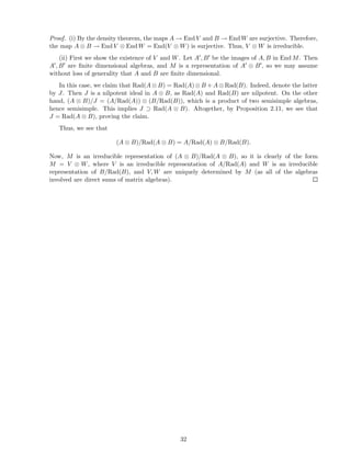
2.10 Representations of tensor products
Let A, B be algebras. Then A ⊗ B is also an algebra, with multiplication (a1 ⊗ b1)(a2 ⊗ b2) =
a1a2 ⊗ b1b2.
Exercise. Show that Matm(k) ⊗ Matn(k) ∼= Matmn(k).
The following theorem describes irreducible finite dimensional representations of A⊗B in terms
of irreducible finite dimensional representations of A and those of B.
Theorem 2.26. (i) Let V be an irreducible finite dimensional representation of A and W an
irreducible finite dimensional representation of B. Then V ⊗ W is an irreducible representation of
A ⊗ B.
(ii) Any irreducible finite dimensional representation M of A ⊗ B has the form (i) for unique
V and W.
Remark 2.27. Part (ii) of the theorem typically fails for infinite dimensional representations;
e.g. it fails when A is the Weyl algebra in characteristic zero. Part (i) also may fail. E.g. let
A = B = V = W = C(x). Then (i) fails, as A ⊗ B is not a field.
31](https://image.slidesharecdn.com/replect-150306080251-conversion-gate01/85/Replect-31-320.jpg)
![3 Representations of finite groups: basic results
Recall that a representation of a group G over a field k is a k-vector space V together with a
group homomorphism ρ : G → GL(V ). As we have explained above, a representation of a group G
over k is the same thing as a representation of its group algebra k[G].
In this section, we begin a systematic development of representation theory of finite groups.
3.1 Maschke’s Theorem
Theorem 3.1. (Maschke) Let G be a finite group and k a field whose characteristic does not divide
|G|. Then:
(i) The algebra k[G] is semisimple.
(ii) There is an isomorphism of algebras ψ : k[G] → ⊕iEndVi defined by g → ⊕ig|Vi , where Vi
are the irreducible representations of G. In particular, this is an isomorphism of representations
of G (where G acts on both sides by left multiplication). Hence, the regular representation k[G]
decomposes into irreducibles as ⊕i dim(Vi)Vi, and one has
|G| =
i
dim(Vi)2
.
(the “sum of squares formula”).
Proof. By Proposition 2.16, (i) implies (ii), and to prove (i), it is sufficient to show that if V is
a finite-dimensional representation of G and W ⊂ V is any subrepresentation, then there exists a
subrepresentation W′ ⊂ V such that V = W ⊕ W′ as representations.
Choose any complement ˆW of W in V . (Thus V = W ⊕ ˆW as vector spaces, but not necessarily
as representations.) Let P be the projection along ˆW onto W, i.e., the operator on V defined by
P|W = Id and P| ˆW = 0. Let
P :=
1
|G|
g∈G
ρ(g)Pρ(g−1
),
where ρ(g) is the action of g on V , and let
W′
= ker P.
Now P|W = Id and P(V ) ⊆ W, so P
2
= P, so P is a projection along W′. Thus, V = W ⊕ W′ as
vector spaces.
Moreover, for any h ∈ G and any y ∈ W′,
Pρ(h)y =
1
|G|
g∈G
ρ(g)Pρ(g−1
h)y =
1
|G|
ℓ∈G
ρ(hℓ)Pρ(ℓ−1
)y = ρ(h)Py = 0,
so ρ(h)y ∈ ker P = W′. Thus, W′ is invariant under the action of G and is therefore a subrepre-
sentation of V . Thus, V = W ⊕ W′ is the desired decomposition into subrepresentations.
The converse to Theorem 3.1(i) also holds.
Proposition 3.2. If k[G] is semisimple, then the characteristic of k does not divide |G|.
33](https://image.slidesharecdn.com/replect-150306080251-conversion-gate01/85/Replect-33-320.jpg)
![Proof. Write k[G] = r
i=1 End Vi, where the Vi are irreducible representations and V1 = k is the
trivial one-dimensional representation. Then
k[G] = k ⊕
r
i=2
End Vi = k ⊕
r
i=2
diVi,
where di = dim Vi. By Schur’s Lemma,
Homk[G](k, k[G]) = kΛ
Homk[G](k[G], k) = kǫ,
for nonzero homomorphisms of representations ǫ : k[G] → k and Λ : k → k[G] unique up to scaling.
We can take ǫ such that ǫ(g) = 1 for all g ∈ G, and Λ such that Λ(1) = g∈G g. Then
ǫ ◦ Λ(1) = ǫ
g∈G
g =
g∈G
1 = |G|.
If |G| = 0, then Λ has no left inverse, as (aǫ) ◦ Λ(1) = 0 for any a ∈ k. This is a contradiction.
Example 3.3. If G = Z/pZ and k has characteristic p, then every irreducible representation of G
over k is trivial (so k[Z/pZ] indeed is not semisimple). Indeed, an irreducible representation of this
group is a 1-dimensional space, on which the generator acts by a p-th root of unity, and every p-th
root of unity in k equals 1, as xp − 1 = (x − 1)p over k.
Problem 3.4. Let G be a group of order pn. Show that every irreducible representation of G over
a field k of characteristic p is trivial.
3.2 Characters
If V is a finite-dimensional representation of a finite group G, then its character χV : G → k
is defined by the formula χV (g) = tr|V (ρ(g)). Obviously, χV (g) is simply the restriction of the
character χV (a) of V as a representation of the algebra A = k[G] to the basis G ⊂ A, so it carries
exactly the same information. The character is a central or class function: χV (g) depends only on
the conjugacy class of g; i.e., χV (hgh−1) = χV (g).
Theorem 3.5. If the characteristic of k does not divide |G|, characters of irreducible representa-
tions of G form a basis in the space Fc(G, k) of class functions on G.
Proof. By the Maschke theorem, k[G] is semisimple, so by Theorem 2.17, the characters are linearly
independent and are a basis of (A/[A, A])∗, where A = k[G]. It suffices to note that, as vector
spaces over k,
(A/[A, A])∗ ∼= {ϕ ∈ Homk(k[G], k) | gh − hg ∈ ker ϕ ∀g, h ∈ G}
∼= {f ∈ Fun(G, k) | f(gh) = f(hg) ∀g, h ∈ G},
which is precisely Fc(G, k).
Corollary 3.6. The number of isomorphism classes of irreducible representations of G equals the
number of conjugacy classes of G (if |G| = 0 in k).
34](https://image.slidesharecdn.com/replect-150306080251-conversion-gate01/85/Replect-34-320.jpg)
![Exercise. Show that if |G| = 0 in k then the number of isomorphism classes of irreducible
representations of G over k is strictly less than the number of conjugacy classes in G.
Hint. Let P = g∈G g ∈ k[G]. Then P2 = 0. So P has zero trace in every finite dimensional
representation of G over k.
Corollary 3.7. Any representation of G is determined by its character if k has characteristic 0;
namely, χV = χW implies V ∼= W.
3.3 Examples
The following are examples of representations of finite groups over C.
1. Finite abelian groups G = Zn1 × · · · × Znk
. Let G∨ be the set of irreducible representations
of G. Every element of G forms a conjugacy class, so |G∨| = |G|. Recall that all irreducible
representations over C (and algebraically closed fields in general) of commutative algebras and
groups are one-dimensional. Thus, G∨ is an abelian group: if ρ1, ρ2 : G → C× are irreducible
representations then so are ρ1(g)ρ2(g) and ρ1(g)−1. G∨ is called the dual or character group
of G.
For given n ≥ 1, define ρ : Zn → C× by ρ(m) = e2πim/n. Then Z∨
n = {ρk : k = 0, . . . , n − 1},
so Z∨
n
∼= Zn. In general,
(G1 × G2 × · · · × Gn)∨
= G∨
1 × G∨
2 × · · · × G∨
n,
so G∨ ∼= G for any finite abelian group G. This isomorphism is, however, noncanonical:
the particular decomposition of G as Zn1 × · · · × Znk
is not unique as far as which elements
of G correspond to Zn1 , etc. is concerned. On the other hand, G ∼= (G∨)∨ is a canonical
isomorphism, given by ϕ : G → (G∨)∨, where ϕ(g)(χ) = χ(g).
2. The symmetric group S3. In Sn, conjugacy classes are determined by cycle decomposition
sizes: two permutations are conjugate if and only if they have the same number of cycles
of each length. For S3, there are 3 conjugacy classes, so there are 3 different irreducible
representations over C. If their dimensions are d1, d2, d3, then d2
1+d2
2+d2
3 = 6, so S3 must have
two 1-dimensional and one 2-dimensional representations. The 1-dimensional representations
are the trivial representation C+ given by ρ(σ) = 1 and the sign representation C− given by
ρ(σ) = (−1)σ.
The 2-dimensional representation can be visualized as representing the symmetries of the
equilateral triangle with vertices 1, 2, 3 at the points (cos 120◦, sin 120◦), (cos 240◦, sin 240◦),
(1, 0) of the coordinate plane, respectively. Thus, for example,
ρ((12)) =
1 0
0 −1
, ρ((123)) =
cos 120◦ − sin 120◦
sin 120◦ cos 120◦ .
To show that this representation is irreducible, consider any subrepresentation V . V must be
the span of a subset of the eigenvectors of ρ((12)), which are the nonzero multiples of (1, 0)
and (0, 1). V must also be the span of a subset of the eigenvectors of ρ((123)), which are
different vectors. Thus, V must be either C2 or 0.
3. The quaternion group Q8 = {±1, ±i, ±j, ±k}, with defining relations
i = jk = −kj, j = ki = −ik, k = ij = −ji, −1 = i2
= j2
= k2
.
35](https://image.slidesharecdn.com/replect-150306080251-conversion-gate01/85/Replect-35-320.jpg)
![If V, W are representations of G, then V ⊗ W is also a representation, via
ρV ⊗W (g) = ρV (g) ⊗ ρW (g).
Therefore, χV ⊗W (g) = χV (g)χW (g).
An interesting problem discussed below is to decompose V ⊗ W (for irreducible V, W) into the
direct sum of irreducible representations.
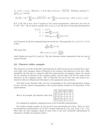
3.5 Orthogonality of characters
We define a positive definite Hermitian inner product on Fc(G, C) (the space of central functions)
by
(f1, f2) =
1
|G|
g∈G
f1(g)f2(g).
The following theorem says that characters of irreducible representations of G form an orthonormal
basis of Fc(G, C) under this inner product.
Theorem 3.8. For any representations V, W
(χV , χW ) = dim HomG(W, V ),
and
(χV , χW ) =
1, if V ∼= W,
0, if V ≇ W
if V, W are irreducible.
Proof. By the definition
(χV , χW ) =
1
|G|
g∈G
χV (g)χW (g) =
1
|G|
g∈G
χV (g)χW ∗ (g)
=
1
|G|
g∈G
χV ⊗W ∗(g) = Tr |V ⊗W ∗ (P),
where P = 1
|G| g∈G g ∈ Z(C[G]). (Here Z(C[G]) denotes the center of C[G]). If X is an irreducible
representation of G then
P|X =
Id, if X = C,
0, X = C.
Therefore, for any representation X the operator P|X is the G-invariant projector onto the subspace
XG of G-invariants in X. Thus,
Tr |V ⊗W ∗(P) = dim HomG(C, V ⊗ W∗
)
= dim(V ⊗ W∗
)G
= dim HomG(W, V ).
37](https://image.slidesharecdn.com/replect-150306080251-conversion-gate01/85/Replect-37-320.jpg)
![Theorem 3.8 gives a powerful method of checking if a given complex representation V of a finite
group G is irreducible. Indeed, it implies that V is irreducible if and only if (χV , χV ) = 1.
Exercise. Let G be a finite group. Let Vi be the irreducible complex representations of G.
For every i, let
ψi =
dim Vi
|G|
g∈G
χVi (g) · g−1
∈ C [G] .
(i) Prove that ψi acts on Vj as the identity if j = i, and as the null map if j = i.
(ii) Prove that ψi are idempotents, i.e., ψ2
i = ψi for any i, and ψiψj = 0 for any i = j.
Hint: In (i), notice that ψi commutes with any element of k [G], and thus acts on Vj as an
intertwining operator. Corollary 1.17 thus yields that ψi acts on Vj as a scalar. Compute this
scalar by taking its trace in Vj.
Here is another “orthogonality formula” for characters, in which summation is taken over irre-
ducible representations rather than group elements.
Theorem 3.9. Let g, h ∈ G, and let Zg denote the centralizer of g in G. Then
V
χV (g)χV (h) =
|Zg| if g is conjugate to h
0, otherwise
where the summation is taken over all irreducible representations of G.
Proof. As noted above, χV (h) = χV ∗ (h), so the left hand side equals (using Maschke’s theorem):
V
χV (g)χV ∗ (h) = Tr|⊕V V ⊗V ∗ (g ⊗ (h∗
)−1
) =
Tr|⊕V EndV (x → gxh−1
) = Tr|C[G](x → gxh−1
).
If g and h are not conjugate, this trace is clearly zero, since the matrix of the operator x → gxh−1
in the basis of group elements has zero diagonal entries. On the other hand, if g and h are in the
same conjugacy class, the trace is equal to the number of elements x such that x = gxh−1, i.e., the
order of the centralizer Zg of g. We are done.
Remark. Another proof of this result is as follows. Consider the matrix U whose rows are
labeled by irreducible representations of G and columns by conjugacy classes, with entries UV,g =
χV (g)/ |Zg|. Note that the conjugacy class of g is G/Zg, thus |G|/|Zg| is the number of elements
conjugate to G. Thus, by Theorem 3.8, the rows of the matrix U are orthonormal. This means
that U is unitary and hence its columns are also orthonormal, which implies the statement.
3.6 Unitary representations. Another proof of Maschke’s theorem for complex
representations
Definition 3.10. A unitary finite dimensional representation of a group G is a representation of G
on a complex finite dimensional vector space V over C equipped with a G-invariant positive definite
Hermitian form4 (, ), i.e., such that ρV (g) are unitary operators: (ρV (g)v, ρV (g)w) = (v, w).
4
We agree that Hermitian forms are linear in the first argument and antilinear in the second one.
38](https://image.slidesharecdn.com/replect-150306080251-conversion-gate01/85/Replect-38-320.jpg)
![4 Representations of finite groups: further results
4.1 Frobenius-Schur indicator
Suppose that G is a finite group and V is an irreducible representation of G over C. We say that
V is
- of complex type, if V ≇ V ∗,
- of real type, if V has a nondegenerate symmetric form invariant under G,
- of quaternionic type, if V has a nondegenerate skew form invariant under G.
Problem 4.1. (a) Show that EndR[G] V is C for V of complex type, Mat2(R) for V of real type,
and H for V of quaternionic type, which motivates the names above.
Hint. Show that the complexification VC of V decomposes as V ⊕ V ∗. Use this to compute the
dimension of EndR[G] V in all three cases. Using the fact that C ⊂ EndR[G] V , prove the result
in the complex case. In the remaining two cases, let B be the invariant bilinear form on V , and
(, ) the invariant positive Hermitian form (they are defined up to a nonzero complex scalar and a
positive real scalar, respectively), and define the operator j : V → V such that B(v, w) = (v, jw).
Show that j is complex antilinear (ji = −ij), and j2 = λ · Id, where λ is a real number, positive in
the real case and negative in the quaternionic case (if B is renormalized, j multiplies by a nonzero
complex number z and j2 by z¯z, as j is antilinear). Thus j can be normalized so that j2 = 1 for
the real case, and j2 = −1 in the quaternionic case. Deduce the claim from this.
(b) Show that V is of real type if and only if V is the complexification of a representation VR
over the field of real numbers.
Example 4.2. For Z/nZ all irreducible representations are of complex type, except the trivial one
and, if n is even, the “sign” representation, m → (−1)m, which are of real type. For S3 all three
irreducible representations C+, C−, C2 are of real type. For S4 there are five irreducible representa-
tions C+, C−, C2, C3
+, C3
−, which are all of real type. Similarly, all five irreducible representations
of A5 – C, C3
+, C3
−, C4, C5 are of real type. As for Q8, its one-dimensional representations are of
real type, and the two-dimensional one is of quaternionic type.
Definition 4.3. The Frobenius-Schur indicator FS(V ) of an irreducible representation V is 0 if it
is of complex type, 1 if it is of real type, and −1 if it is of quaternionic type.
Theorem 4.4. (Frobenius-Schur) The number of involutions (=elements of order ≤ 2) in G is
equal to V dim(V )FS(V ), i.e., the sum of dimensions of all representations of G of real type
minus the sum of dimensions of its representations of quaternionic type.
Proof. Let A : V → V have eigenvalues λ1, λ2, . . . , λn. We have
Tr|S2V (A ⊗ A) =
i≤j
λiλj
Tr|Λ2V (A ⊗ A) =
i<j
λiλj
Thus,
Tr|S2V (A ⊗ A) − Tr|Λ2V (A ⊗ A) =
1≤i≤n
λ2
i = Tr(A2
).
47](https://image.slidesharecdn.com/replect-150306080251-conversion-gate01/85/Replect-47-320.jpg)
![Thus for g ∈ G we have
χV (g2
) = χS2V (g) − χΛ2V (g)
Therefore,
|G|−1
χV (
g∈G
g2
) = χS2V (P)−χ∧2V (P) = dim(S2
V )G
−dim(∧2
V )G
=
1, if V is of real type
−1, if V is of quaternionic type
0, if V is of complex type
Finally, the number of involutions in G equals
1
|G|
V
dim V χV (
g∈G
g2
) =
real V
dim V −
quat V
dim V.
Corollary 4.5. Assume that all representations of a finite group G are defined over real numbers
(i.e., all complex representations of G are obtained by complexifying real representations). Then
the sum of dimensions of irreducible representations of G equals the number of involutions in G.
Exercise. Show that any nontrivial finite group of odd order has an irreducible representation
which is not defined over R (i.e., not realizable by real matrices).
4.2 Frobenius determinant
Enumerate the elements of a finite group G as follows: g1, g2, . . . , gn. Introduce n variables indexed
with the elements of G :
xg1 , xg2 , . . . , xgn .
Definition 4.6. Consider the matrix XG with entries aij = xgigj . The determinant of XG is some
polynomial of degree n of xg1 , xg2 , . . . , xgn that is called the Frobenius determinant.
The following theorem, discovered by Dedekind and proved by Frobenius, became the starting
point for creation of representation theory (see [Cu]).
Theorem 4.7.
det XG =
r
j=1
Pj(x)deg Pj
for some pairwise non-proportional irreducible polynomials Pj(x), where r is the number of conju-
gacy classes of G.
We will need the following simple lemma.
Lemma 4.8. Let Y be an n × n matrix with entries yij. Then det Y is an irreducible polynomial
of {yij}.
Proof. Let Y = t·Id+ n
i=1 xiEi,i+1, where i+1 is computed modulo n, and Ei,j are the elementary
matrices. Then det(Y ) = tn − (−1)nx1...xn, which is obviously irreducible. Hence det(Y ) is
irreducible (since factors of a homogeneous polynomial are homogeneous).
Now we are ready to proceed to the proof of Theorem 4.7.
48](https://image.slidesharecdn.com/replect-150306080251-conversion-gate01/85/Replect-48-320.jpg)
![Proof. Let V = C[G] be the regular representation of G. Consider the operator-valued polynomial
L(x) =
g∈G
xgρ(g),
where ρ(g) ∈ EndV is induced by g. The action of L(x) on an element h ∈ G is
L(x)h =
g∈G
xgρ(g)h =
g∈G
xggh =
z∈G
xzh−1 z
So the matrix of the linear operator L(x) in the basis g1, g2, . . . , gn is XG with permuted columns
and hence has the same determinant up to sign.
Further, by Maschke’s theorem, we have
detV L(x) =
r
i=1
(detVi L(x))dim Vi
,
where Vi are the irreducible representations of G. We set Pi = detVi L(x). Let {eim} be bases of Vi
and Ei,jk ∈ End Vi be the matrix units in these bases. Then {Ei,jk} is a basis of C[G] and
L(x)|Vi =
j,k
yi,jkEi,jk,
where yi,jk are new coordinates on C[G] related to xg by a linear transformation. Then
Pi(x) = det |Vi L(x) = det(yi,jk)
Hence, Pi are irreducible (by Lemma 4.8) and not proportional to each other (as they depend on
different collections of variables yi,jk). The theorem is proved.
4.3 Algebraic numbers and algebraic integers
We are now passing to deeper results in representation theory of finite groups. These results require
the theory of algebraic numbers, which we will now briefly review.
Definition 4.9. z ∈ C is an algebraic number (respectively, an algebraic integer), if z is a
root of a monic polynomial with rational (respectively, integer) coefficients.
Definition 4.10. z ∈ C is an algebraic number, (respectively, an algebraic integer), if z is an
eigenvalue of a matrix with rational (respectively, integer) entries.
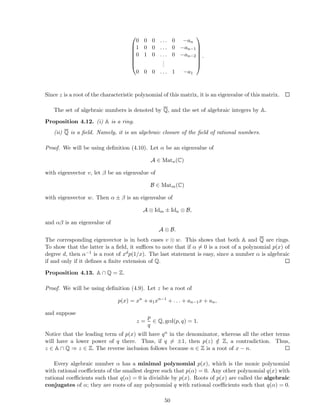
Proposition 4.11. Definitions (4.9) and (4.10) are equivalent.
Proof. To show (4.10) ⇒ (4.9), notice that z is a root of the characteristic polynomial of the matrix
(a monic polynomial with rational, respectively integer, coefficients).
To show (4.9) ⇒ (4.10), suppose z is a root of
p(x) = xn
+ a1xn−1
+ . . . + an−1x + an.
Then the characteristic polynomial of the following matrix (called the companion matrix) is
p(x):
49](https://image.slidesharecdn.com/replect-150306080251-conversion-gate01/85/Replect-49-320.jpg)
![Note that any algebraic conjugate of an algebraic integer is obviously also an algebraic inte-
ger. Therefore, by the Vieta theorem, the minimal polynomial of an algebraic integer has integer
coefficients.
Below we will need the following lemma:
Lemma 4.14. If α1, ..., αm are algebraic numbers, then all algebraic conjugates to α1 + ... + αm
are of the form α′
1 + ... + α′
m, where α′
i are some algebraic conjugates of αi.
Proof. It suffices to prove this for two summands. If αi are eigenvalues of rational matrices Ai of
smallest size (i.e., their characteristic polynomials are the minimal polynomials of αi), then α1 +α2
is an eigenvalue of A := A1 ⊗ Id + Id ⊗ A2. Therefore, so is any algebraic conjugate to α1 + α2.
But all eigenvalues of A are of the form α′
1 + α′
2, so we are done.
Problem 4.15. (a) Show that for any finite group G there exists a finite Galois extension K ⊂ C
of Q such that any finite dimensional complex representation of G has a basis in which the matrices
of the group elements have entries in K.
Hint. Consider the representations of G over the field Q of algebraic numbers.
(b) Show that if V is an irreducible complex representation of a finite group G of dimension
> 1 then there exists g ∈ G such that χV (g) = 0.
Hint: Assume the contrary. Use orthonormality of characters to show that the arithmetic mean
of the numbers |χV (g)|2 for g = 1 is < 1. Deduce that their product β satisfies 0 < β < 1.
Show that all conjugates of β satisfy the same inequalities (consider the Galois conjugates of the
representation V , i.e. representations obtained from V by the action of the Galois group of K over
Q on the matrices of group elements in the basis from part (a)). Then derive a contradiction.
Remark. Here is a modification of this argument, which does not use (a). Let N = |G|. For
any 0 < j < N coprime to N, show that the map g → gj is a bijection G → G. Deduce that
g=1 |χV (gj)|2 = β. Then show that β ∈ K := Q(ζ), ζ = e2πi/N , and does not change under the
automorphism of K given by ζ → ζj. Deduce that β is an integer, and derive a contradiction.
4.4 Frobenius divisibility
Theorem 4.16. Let G be a finite group, and let V be an irreducible representation of G over C.
Then
dim V divides |G|.
Proof. Let C1, C2, . . . , Cn be the conjugacy classes of G. Set
λi = χV (gCi )
|Ci|
dim V
,
where gCi is a representative of Ci.
Proposition 4.17. The numbers λi are algebraic integers for all i.
Proof. Let C be a conjugacy class in G, and P = h∈C h. Then P is a central element of Z[G], so it
acts on V by some scalar λ, which is an algebraic integer (indeed, since Z[G] is a finitely generated
Z-module, any element of Z[G] is integral over Z, i.e., satisfies a monic polynomial equation with
integer coefficients). On the other hand, taking the trace of P in V , we get |C|χV (g) = λ dim V ,
g ∈ C, so λ = |C|χV (g)
dim V .
51](https://image.slidesharecdn.com/replect-150306080251-conversion-gate01/85/Replect-51-320.jpg)
![Now, consider
i
λiχV (gCi ).
This is an algebraic integer, since:
(i) λi are algebraic integers by Proposition 4.17,
(ii) χV (gCi ) is a sum of roots of unity (it is the sum of eigenvalues of the matrix of ρ(gCi ), and
since g
|G|
Ci
= e in G, the eigenvalues of ρ(gCi ) are roots of unity), and
(iii) A is a ring (Proposition 4.12).
On the other hand, from the definition of λi,
Ci
λiχV (gCi ) =
i
|Ci|χV (gCi )χV (gCi )
dim V
.
Recalling that χV is a class function, this is equal to
g∈G
χV (g)χV (g)
dim V
=
|G|(χV , χV )
dim V
.
Since V is an irreducible representation, (χV , χV ) = 1, so
Ci
λiχV (gCi ) =
|G|
dim V
.
Since |G|
dim V ∈ Q and Ci
λiχV (gCi ) ∈ A, by Proposition 4.13 |G|
dim V ∈ Z.
4.5 Burnside’s Theorem
Definition 4.18. A group G is called solvable if there exists a series of nested normal subgroups
{e} = G1 ⊳ G2 ⊳ . . . ⊳ Gn = G
where Gi+1/Gi is abelian for all 1 ≤ i ≤ n − 1.
Remark 4.19. Such groups are called solvable because they first arose as Galois groups of poly-
nomial equations which are solvable in radicals.
Theorem 4.20 (Burnside). Any group G of order paqb, where p and q are prime and a, b ≥ 0, is
solvable.
This famous result in group theory was proved by the British mathematician William Burnside
in the early 20-th century, using representation theory (see [Cu]). Here is this proof, presented in
modern language.
Before proving Burnside’s theorem we will prove several other results which are of independent
interest.
Theorem 4.21. Let V be an irreducible representation of a finite group G and let C be a conjugacy
class of G with gcd(|C|, dim(V )) = 1. Then for any g ∈ C, either χV (g) = 0 or g acts as a scalar
on V .
52](https://image.slidesharecdn.com/replect-150306080251-conversion-gate01/85/Replect-52-320.jpg)
![and the action g(f)(x) = f(xg) ∀g ∈ G.
Remark 4.29. In fact, IndG
HV is naturally isomorphic to HomH(k[G], V ).
Let us check that IndG
HV is indeed a representation:
g(f)(hx) = f(hxg) = ρV (h)f(xg) = ρV (h)g(f)(x), and g(g′(f))(x) = g′(f)(xg) = f(xgg′) =
(gg′)(f)(x) for any g, g′, x ∈ G and h ∈ H.
Remark 4.30. Notice that if we choose a representative xσ from every right H-coset σ of G, then
any f ∈ IndG
HV is uniquely determined by {f(xσ)}.
Because of this,
dim(IndG
HV ) = dim V ·
|G|
|H|
.
Problem 4.31. Check that if K ⊂ H ⊂ G are groups and V a representation of K then IndG
H IndH
KV
is isomorphic to IndG
KV .
Exercise. Let K ⊂ G be finite groups, and χ : K → C∗ be a homomorphism. Let Cχ be the
corresponding 1-dimensional representation of K. Let
eχ =
1
|K|
g∈K
χ(g)−1
g ∈ C[K]
be the idempotent corresponding to χ. Show that the G-representation IndG
KCχ is naturally iso-
morphic to C[G]eχ (with G acting by left multiplication).
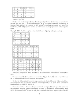
4.9 The Mackey formula
Let us now compute the character χ of IndG
HV . In each right coset σ ∈ HG, choose a representative
xσ.
Theorem 4.32. (The Mackey formula) One has
χ(g) =
σ∈HG:xσgx−1
σ ∈H
χV (xσgx−1
σ ).
Remark. If the characteristic of the ground field k is relatively prime to |H|, then this formula
can be written as
χ(g) =
1
|H|
x∈G:xgx−1∈H
χV (xgx−1
).
Proof. For a right H-coset σ of G, let us define
Vσ = {f ∈ IndG
H V |f(g) = 0 ∀g ∈ σ}.
Then one has
IndG
HV =
σ
Vσ,
and so
χ(g) =
σ
χσ(g),
55](https://image.slidesharecdn.com/replect-150306080251-conversion-gate01/85/Replect-55-320.jpg)
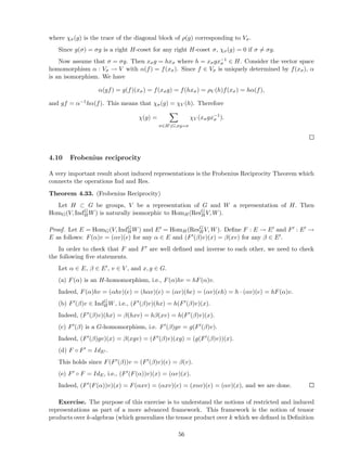
![1.48). In particular, this understanding will lead us to a new proof of the Frobenius reciprocity
and to some analogies between induction and restriction.
Throughout this exercise, we will use the notation and results of the Exercise in Section 1.10.
Let G be a finite group and H ⊂ G a subgroup. We consider k [G] as a (k [H] , k [G])-bimodule
(both module structures are given by multiplication inside k [G]). We denote this bimodule by
k [G]1. On the other hand, we can also consider k [G] as a (k [G] , k [H])-bimodule (again, both
module structures are given by multiplication). We denote this bimodule by k [G]2.
(a) Let V be a representation of G. Then, V is a left k [G]-module, thus a (k [G] , k)-bimodule.
Thus, the tensor product k [G]1 ⊗k[G] V is a (k [H] , k)-bimodule, i. e., a left k [H]-module. Prove
that this tensor product is isomorphic to ResG
HV as a left k [H]-module. The isomorphism ResG
HV →
k [G]1 ⊗k[G] V is given by v → 1 ⊗k[G] v for every v ∈ ResG
HV .
(b) Let W be a representation of H. Then, W is a left k [H]-module, thus a (k [H] , k)-
bimodule. Then, IndG
HW ∼= HomH (k [G] , W), according to Remark 4.30. In other words, IndG
HW ∼=
Homk[H] (k [G]1 , W). Now, use part (b) of the Exercise in Section 1.10 to conclude Theorem 4.33.
(c) Let V be a representation of G. Then, V is a left k [G]-module, thus a (k [G] , k)-bimodule.
Prove that not only k [G]1 ⊗k[G] V , but also Homk[G] (k [G]2 , V ) is isomorphic to ResG
HV as a left
k [H]-module. The isomorphism Homk[G] (k [G]2 , V ) → ResG
HV is given by f → f (1) for every
f ∈ Homk[G] (k [G]2 , V ).
(d) Let W be a representation of H. Then, W is a left k [H]-module, thus a (k [H] , k)-
bimodule. Show that IndG
HW is not only isomorphic to Homk[H] (k [G]1 , W), but also isomorphic to
k [G]2⊗k[H]W. The isomorphism Homk[H] (k [G]1 , W) → k [G]2⊗k[H]W is given by f → g∈P g−1⊗k[H]
f (g) for every f ∈ Homk[H] (k [G]1 , W), where P is a set of distinct representatives for the right
H-cosets in G. (This isomorphism is independent of the choice of representatives.)
(e) Let V be a representation of G and W a representation of H. Use (b) to prove that
HomG IndG
H W, V is naturally isomorphic to HomH W, ResG
H V .
(f) Let V be a representation of H. Prove that IndG
H (V ∗) ∼= IndG
HV
∗
as representations of
G. [Hint: Write IndG
HV as k [G]2 ⊗k[H] V and write IndG
H (V ∗) as Homk[H] (k [G]1 , V ∗). Prove
that the map Homk[H] (k [G]1 , V ∗) × IndG
H (V ∗) → k given by f, x ⊗k[H] v → (f (Sx)) (v) is
a nondegenerate G-invariant bilinear form, where S : k [G] → k [G] is the linear map defined by
Sg = g−1 for every g ∈ G.]
4.11 Examples
Here are some examples of induced representations (we use the notation for representations from
the character tables).
1. Let G = S3, H = Z2. Using the Frobenius reciprocity, we obtain: IndG
HC+ = C2 ⊕ C+,
IndG
HC− = C2 ⊕ C−.
2. Let G = S3, H = Z3. Then we obtain IndG
H C+ = C+ ⊕ C−, IndG
H Cǫ = IndG
HCǫ2 = C2.
3. Let G = S4, H = S3. Then IndG
HC+ = C+⊕C3
−, IndG
HC− = C−⊕C3
+, IndG
HC2 = C2⊕C3
−⊕C3
+.
Problem 4.34. Compute the decomposition into irreducibles of all the representations of A5 in-
duced from all the irreducible representations of
57](https://image.slidesharecdn.com/replect-150306080251-conversion-gate01/85/Replect-57-320.jpg)
![(a) Z2
(b) Z3
(c) Z5
(d) A4
(e) Z2 × Z2
4.12 Representations of Sn
In this subsection we give a description of the representations of the symmetric group Sn for any
n.
Definition 4.35. A partition λ of n is a representation of n in the form n = λ1 + λ2 + ... + λp,
where λi are positive integers, and λi ≥ λi+1.
To such λ we will attach a Young diagram Yλ, which is the union of rectangles −i ≤ y ≤ −i+1,
0 ≤ x ≤ λi in the coordinate plane, for i = 1, ..., p. Clearly, Yλ is a collection of n unit squares. A
Young tableau corresponding to Yλ is the result of filling the numbers 1, ..., n into the squares of
Yλ in some way (without repetitions). For example, we will consider the Young tableau Tλ obtained
by filling in the numbers in the increasing order, left to right, top to bottom.
We can define two subgroups of Sn corresponding to Tλ:
1. The row subgroup Pλ: the subgroup which maps every element of {1, ..., n} into an element
standing in the same row in Tλ.
2. The column subgroup Qλ: the subgroup which maps every element of {1, ..., n} into an
element standing in the same column in Tλ.
Clearly, Pλ ∩ Qλ = {1}.
Define the Young projectors:
aλ :=
1
|Pλ|
g∈Pλ
g,
bλ :=
1
|Qλ|
g∈Qλ
(−1)g
g,
where (−1)g denotes the sign of the permutation g. Set cλ = aλbλ. Since Pλ ∩ Qλ = {1}, this
element is nonzero.
The irreducible representations of Sn are described by the following theorem.
Theorem 4.36. The subspace Vλ := C[Sn]cλ of C[Sn] is an irreducible representation of Sn under
left multiplication. Every irreducible representation of Sn is isomorphic to Vλ for a unique λ.
The modules Vλ are called the Specht modules.
The proof of this theorem is given in the next subsection.
Example 4.37.
For the partition λ = (n), Pλ = Sn, Qλ = {1}, so cλ is the symmetrizer, and hence Vλ is the trivial
representation.
58](https://image.slidesharecdn.com/replect-150306080251-conversion-gate01/85/Replect-58-320.jpg)
![For the partition λ = (1, ..., 1), Qλ = Sn, Pλ = {1}, so cλ is the antisymmetrizer, and hence Vλ is
the sign representation.
n = 3. For λ = (2, 1), Vλ = C2.
n = 4. For λ = (2, 2), Vλ = C2; for λ = (3, 1), Vλ = C3
−; for λ = (2, 1, 1), Vλ = C3
+.
Corollary 4.38. All irreducible representations of Sn can be given by matrices with rational entries.
Problem 4.39. Find the sum of dimensions of all irreducible representations of the symmetric
group Sn.
Hint. Show that all irreducible representations of Sn are real, i.e., admit a nondegenerate
invariant symmetric form. Then use the Frobenius-Schur theorem.
4.13 Proof of Theorem 4.36
Lemma 4.40. Let x ∈ C[Sn]. Then aλxbλ = ℓλ(x)cλ, where ℓλ is a linear function.
Proof. If g ∈ PλQλ, then g has a unique representation as pq, p ∈ Pλ, q ∈ Qλ, so aλgbλ = (−1)qcλ.
Thus, to prove the required statement, we need to show that if g is a permutation which is not in
PλQλ then aλgbλ = 0.
To show this, it is sufficient to find a transposition t such that t ∈ Pλ and g−1tg ∈ Qλ; then
aλgbλ = aλtgbλ = aλg(g−1
tg)bλ = −aλgbλ,
so aλgbλ = 0. In other words, we have to find two elements i, j standing in the same row in the
tableau T = Tλ, and in the same column in the tableau T′ = gT (where gT is the tableau of the
same shape as T obtained by permuting the entries of T by the permutation g). Thus, it suffices to
show that if such a pair does not exist, then g ∈ PλQλ, i.e., there exists p ∈ Pλ, q′ ∈ Q′
λ := gQλg−1
such that pT = q′T′ (so that g = pq−1, q = g−1q′g ∈ Qλ).
Any two elements in the first row of T must be in different columns of T′, so there exists q′
1 ∈ Q′
λ
which moves all these elements to the first row. So there is p1 ∈ Pλ such that p1T and q′
1T′ have
the same first row. Now do the same procedure with the second row, finding elements p2, q′
2 such
that p2p1T and q′
2q′
1T′ have the same first two rows. Continuing so, we will construct the desired
elements p, q′. The lemma is proved.
Let us introduce the lexicographic ordering on partitions: λ > µ if the first nonvanishing
λi − µi is positive.
Lemma 4.41. If λ > µ then aλC[Sn]bµ = 0.
Proof. Similarly to the previous lemma, it suffices to show that for any g ∈ Sn there exists a
transposition t ∈ Pλ such that g−1tg ∈ Qµ. Let T = Tλ and T′ = gTµ. We claim that there are
two integers which are in the same row of T and the same column of T′. Indeed, if λ1 > µ1, this is
clear by the pigeonhole principle (already for the first row). Otherwise, if λ1 = µ1, like in the proof
of the previous lemma, we can find elements p1 ∈ Pλ, q′
1 ∈ gQµg−1 such that p1T and q′
1T′ have the
same first row, and repeat the argument for the second row, and so on. Eventually, having done
i−1 such steps, we’ll have λi > µi, which means that some two elements of the i-th row of the first
tableau are in the same column of the second tableau, completing the proof.
59](https://image.slidesharecdn.com/replect-150306080251-conversion-gate01/85/Replect-59-320.jpg)
![Lemma 4.42. cλ is proportional to an idempotent. Namely, c2
λ = n!
dim Vλ
cλ.
Proof. Lemma 4.40 implies that c2
λ is proportional to cλ. Also, it is easy to see that the trace of
cλ in the regular representation is n! (as the coefficient of the identity element in cλ is 1). This
implies the statement.
Lemma 4.43. Let A be an algebra and e be an idempotent in A. Then for any left A-module M,
one has HomA(Ae, M) ∼= eM (namely, x ∈ eM corresponds to fx : Ae → M given by fx(a) = ax,
a ∈ Ae).
Proof. Note that 1 − e is also an idempotent in A. Thus the statement immediately follows from
the fact that HomA(A, M) ∼= M and the decomposition A = Ae ⊕ A(1 − e).
Now we are ready to prove Theorem 4.36. Let λ ≥ µ. Then by Lemmas 4.42, 4.43
HomSn (Vλ, Vµ) = HomSn (C[Sn]cλ, C[Sn]cµ) = cλC[Sn]cµ.
The latter space is zero for λ > µ by Lemma 4.41, and 1-dimensional if λ = µ by Lemmas 4.40
and 4.42. Therefore, Vλ are irreducible, and Vλ is not isomorphic to Vµ if λ = µ. Since the number
of partitions equals the number of conjugacy classes in Sn, the representations Vλ exhaust all the
irreducible representations of Sn. The theorem is proved.
4.14 Induced representations for Sn
Denote by Uλ the representation IndSn
Pλ
C. It is easy to see that Uλ can be alternatively defined as
Uλ = C[Sn]aλ.
Proposition 4.44. Hom(Uλ, Vµ) = 0 for µ < λ, and dim Hom(Uλ, Vλ) = 1. Thus, Uλ =
⊕µ≥λKµλVµ, where Kµλ are nonnegative integers and Kλλ = 1.
Definition 4.45. The integers Kµλ are called the Kostka numbers.
Proof. By Lemmas 4.42 and 4.43,
Hom(Uλ, Vµ) = Hom(C[Sn]aλ, C[Sn]aµbµ) = aλC[Sn]aµbµ,
and the result follows from Lemmas 4.40 and 4.41.
Now let us compute the character of Uλ. Let Ci be the conjugacy class in Sn having il cycles
of length l for all l ≥ 1 (here i is a shorthand notation for (i1, ..., il, ...)). Also let x1, ..., xN be
variables, and let
Hm(x) =
i
xm
i
be the power sum polynomials.
Theorem 4.46. Let N ≥ p (where p is the number of parts of λ). Then χUλ
(Ci) is the coefficient6
of xλ := x
λj
j in the polynomial
m≥1
Hm(x)im
.
6
If j > p, we define λj to be zero.
60](https://image.slidesharecdn.com/replect-150306080251-conversion-gate01/85/Replect-60-320.jpg)
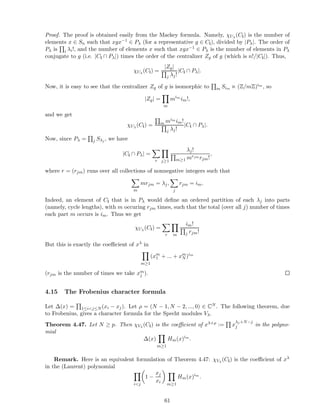
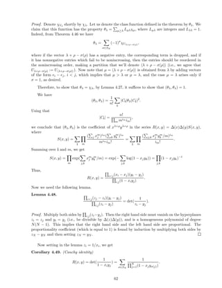
![Corollary 4.49 easily implies that the coefficient of xλ+ρyλ+ρ is 1. Indeed, if σ = 1 is a permu-
tation in SN , the coefficient of this monomial in 1Q
(1−xj yσ(j)) is obviously zero.
Remark. For partitions λ and µ of n, let us say that λ µ or µ λ if µ − λ is a sum of
vectors of the form ei − ej, i < j (called positive roots). This is a partial order, and µ λ implies
µ ≥ λ. It follows from Theorem 4.47 and its proof that
χλ = ⊕µ λKµλχUµ .
This implies that the Kostka numbers Kµλ vanish unless µ λ.
4.16 Problems
In the following problems, we do not make a distinction between Young diagrams and partitions.
Problem 4.50. For a Young diagram µ, let A(µ) be the set of Young diagrams obtained by adding
a square to µ, and R(µ) be the set of Young diagrams obtained by removing a square from µ.
(a) Show that ResSn
Sn−1
Vµ = ⊕λ∈R(µ)Vλ.
(b) Show that IndSn
Sn−1
Vµ = ⊕λ∈A(µ)Vλ.
Problem 4.51. The content c(λ) of a Young diagram λ is the sum j
λj
i=1(i − j). Let C =
i<j(ij) ∈ C[Sn] be the sum of all transpositions. Show that C acts on the Specht module Vλ by
multiplication by c(λ).
Problem 4.52. (a) Let V be any finite dimensional representation of Sn. Show that the element
E := (12) + ... + (1n) is diagonalizable and has integer eigenvalues on V , which are between 1 − n
and n − 1.
Represent E as Cn − Cn−1, where Cn = C is the element from Problem 4.51.
(b) Show that the element (12)+...+(1n) acts on Vλ by a scalar if and only if λ is a rectangular
Young diagram, and compute this scalar.
4.17 The hook length formula
Let us use the Frobenius character formula to compute the dimension of Vλ. According to the
character formula, dim Vλ is the coefficient of xλ+ρ in ∆(x)(x1 + ... + xN )n. Let lj = λj + N − j.
Then, using the determinant formula for ∆(x) and expanding the determinant as a sum over
permutations, we get
dim Vλ =
s∈SN :lj≥N−s(j)
(−1)s n!
j(lj − N + s(j))!
=
n!
l1!...lN !
s∈SN
(−1)s
j
lj(lj−1)...(lj−N+s(j)+1) =
n!
j lj!
det(lj(lj − 1)...(lj − N + i + 1)).
Using column reduction and the Vandermonde determinant formula, we see from this expression
that
dim Vλ =
n!
j lj!
det(lN−i
j ) =
n!
j lj!
1≤i<j≤N
(li − lj) (5)
63](https://image.slidesharecdn.com/replect-150306080251-conversion-gate01/85/Replect-63-320.jpg)
![(where N ≥ p).
In this formula, there are many cancelations. After making some of these cancelations, we
obtain the hook length formula. Namely, for a square (i, j) in a Young diagram λ (i, j ≥ 1, i ≤ λj),
define the hook of (i, j) to be the set of all squares (i′, j′) in λ with i′ ≥ i, j′ = j or i′ = i, j′ ≥ j.
Let h(i, j) be the length of the hook of i, j, i.e., the number of squares in it.
Theorem 4.53. (The hook length formula) One has
dim Vλ =
n!
i≤λj
h(i, j)
.
Proof. The formula follows from formula (5). Namely, note that
l1!
1<j≤N (l1 − lj)
=
1≤k≤l1,k=l1−lj
k.
It is easy to see that the factors in this product are exactly the hooklengths h(i, 1). Now delete the
first row of the diagram and proceed by induction.
4.18 Schur-Weyl duality for gl(V )
We start with a simple result which is called the Double Centralizer Theorem.
Theorem 4.54. Let A, B be two subalgebras of the algebra End E of endomorphisms of a finite
dimensional vector space E, such that A is semisimple, and B = EndA E. Then:
(i) A = EndB E (i.e., the centralizer of the centralizer of A is A);
(ii) B is semisimple;
(iii) as a representation of A ⊗ B, E decomposes as E = ⊕i∈IVi ⊗ Wi, where Vi are all the
irreducible representations of A, and Wi are all the irreducible representations of B. In particular,
we have a natural bijection between irreducible representations of A and B.
Proof. Since A is semisimple, we have a natural decomposition E = ⊕i∈IVi ⊗ Wi, where Wi :=
HomA(Vi, E), and A = ⊕i End Vi. Therefore, by Schur’s lemma, B = EndA(E) is naturally identi-
fied with ⊕i End(Wi). This implies all the statements of the theorem.
We will now apply Theorem 4.54 to the following situation: E = V ⊗n, where V is a finite
dimensional vector space over a field of characteristic zero, and A is the image of C[Sn] in End E.
Let us now characterize the algebra B. Let gl(V ) be End V regarded as a Lie algebra with operation
ab − ba.
Theorem 4.55. The algebra B = EndA E is the image of the universal enveloping algebra U(gl(V ))
under its natural action on E. In other words, B is generated by elements of the form
∆n(b) := b ⊗ 1 ⊗ ... ⊗ 1 + 1 ⊗ b ⊗ ... ⊗ 1 + ... + 1 ⊗ 1 ⊗ ... ⊗ b,
b ∈ gl(V ).
Proof. Clearly, the image of U(gl(V )) is contained in B, so we just need to show that any element
of B is contained in the image of U(gl(V )). By definition, B = Sn End V , so the result follows from
part (ii) of the following lemma.
64](https://image.slidesharecdn.com/replect-150306080251-conversion-gate01/85/Replect-64-320.jpg)
![Lemma 4.56. Let k be a field of characteristic zero.
(i) For any finite dimensional vector space U over k, the space SnU is spanned by elements of
the form u ⊗ ... ⊗ u, u ∈ U.
(ii) For any algebra A over k, the algebra SnA is generated by elements ∆n(a), a ∈ A.
Proof. (i) The space SnU is an irreducible representation of GL(U) (Problem 3.19). The subspace
spanned by u ⊗ ... ⊗ u is a nonzero subrepresentation, so it must be everything.
(ii) By the fundamental theorem on symmetric functions, there exists a polynomial P with
rational coefficients such that P(H1(x), ..., Hn(x)) = x1...xn (where x = (x1, ..., xn)). Then
P(∆n(a), ∆n(a2
), ..., ∆n(an
)) = a ⊗ ... ⊗ a.
The rest follows from (i).
Now, the algebra A is semisimple by Maschke’s theorem, so the double centralizer theorem
applies, and we get the following result, which goes under the name “Schur-Weyl duality”.
Theorem 4.57. (i) The image A of C[Sn] and the image B of U(gl(V )) in End(V ⊗n) are central-
izers of each other.
(ii) Both A and B are semisimple. In particular, V ⊗n is a semisimple gl(V )-module.
(iii) We have a decomposition of A ⊗ B-modules V ⊗n = ⊕λVλ ⊗ Lλ, where the summation
is taken over partitions of n, Vλ are Specht modules for Sn, and Lλ are some distinct irreducible
representations of gl(V ) or zero.
4.19 Schur-Weyl duality for GL(V )
The Schur-Weyl duality for the Lie algebra gl(V ) implies a similar statement for the group GL(V ).
Proposition 4.58. The image of GL(V ) in End(V ⊗n) spans B.
Proof. Denote the span of g⊗n, g ∈ GL(V ), by B′. Let b ∈ End V be any element.
We claim that B′ contains b⊗n. Indeed, for all values of t but finitely many, t·Id+b is invertible,
so (t · Id + b)⊗n belongs to B′. This implies that this is true for all t, in particular for t = 0, since
(t · Id + b)⊗n is a polynomial in t.
The rest follows from Lemma 4.56.
Corollary 4.59. As a representation of Sn × GL(V ), V ⊗n decomposes as ⊕λVλ ⊗ Lλ, where
Lλ = HomSn (Vλ, V ⊗n) are distinct irreducible representations of GL(V ) or zero.
Example 4.60. If λ = (n) then Lλ = SnV , and if λ = (1n) (n copies of 1) then Lλ = ∧nV . It was
shown in Problem 3.19 that these representations are indeed irreducible (except that ∧nV is zero
if n > dim V ).
65](https://image.slidesharecdn.com/replect-150306080251-conversion-gate01/85/Replect-65-320.jpg)
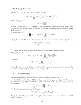
![Theorem 4.63. (Weyl character formula) The representation Lλ is zero if and only if N < p,
where p is the number of parts of λ. If N ≥ p, the character of Lλ is the Schur polynomial Sλ(x).
Therefore, the dimension of Lλ is given by the formula
dim Lλ =
1≤i<j≤N
λi − λj + j − i
j − i
This shows that irreducible representations of GL(V ) which occur in V ⊗n for some n are labeled
by Young diagrams with any number of squares but at most N = dim V rows.
Proposition 4.64. The representation Lλ+1N (where 1N = (1, 1, ..., 1) ∈ ZN ) is isomorphic to
Lλ ⊗ ∧N V .
Proof. Indeed, Lλ ⊗ ∧N V ⊂ V ⊗n ⊗ ∧N V ⊂ V ⊗n+N , and the only component of V ⊗n+N that has
the same character as Lλ ⊗ ∧N V is Lλ+1N . This implies the statement.
4.22 Polynomial representations of GL(V )
Definition 4.65. We say that a finite dimensional representation Y of GL(V ) is polynomial (or
algebraic, or rational) if its matrix elements are polynomial functions of the entries of g, g−1,
g ∈ GL(V ) (i.e., belong to k[gij][1/ det(g)]).
For example, V ⊗n and hence all Lλ are polynomial. Also define Lλ−r·1N := Lλ ⊗(∧N V ∗)⊗r (this
definition makes sense by Proposition 4.64). This is also a polynomial representation. Thus we
have attached a unique irreducible polynomial representation Lλ of GL(V ) = GLN to any sequence
(λ1, ..., λN ) of integers (not necessarily positive) such that λ1 ≥ ... ≥ λN . This sequence is called
the highest weight of Lλ.
Theorem 4.66. (i) Every finite dimensional polynomial representation of GL(V ) is completely
reducible, and decomposes into summands of the form Lλ (which are pairwise non-isomorphic).
(ii) (the Peter-Weyl theorem for GL(V )). Let R be the algebra of polynomial functions on
GL(V ). Then as a representation of GL(V ) × GL(V ) (with action (ρ(g, h)φ)(x) = φ(g−1xh),
g, h, x ∈ GL(V ), φ ∈ R), R decomposes as
R = ⊕λL∗
λ ⊗ Lλ,
where the summation runs over all λ.
Proof. (i) Let Y be a polynomial representation of GL(V ). We have an embedding ξ : Y → Y ⊗ R
given by (u, ξ(v))(g) := u(gv), u ∈ V ∗. It is easy to see that ξ is a homomorphism of representations
(where the action of GL(V ) on the first component of Y ⊗ R is trivial). Thus, it suffices to prove
the theorem for a subrepresentation Y ⊂ Rm. Now, every element of R is a polynomial of gij
times a nonpositive power of det(g). Thus, R is a quotient of a direct sum of representations of the
form Sr(V ⊗ V ∗) ⊗ (∧N V ∗)⊗s. So we may assume that Y is contained in a quotient of a (finite)
direct sum of such representations. As V ∗ = ∧N−1V ⊗ ∧N V ∗, Y is contained in a direct sum of
representations of the form V ⊗n ⊗ (∧N V ∗)⊗s, and we are done.
(ii) Let Y be a polynomial representation of GL(V ), and let us regard R as a representation
of GL(V ) via (ρ(h)φ)(x) = φ(xh). Then HomGL(V )(Y, R) is the space of polynomial functions
on GL(V ) with values in Y ∗, which are GL(V )-equivariant. This space is naturally identified
67](https://image.slidesharecdn.com/replect-150306080251-conversion-gate01/85/Replect-67-320.jpg)
![with Y ∗. Taking into account the proof of (i), we deduce that R has the required decomposition,
which is compatible with the second action of GL(V ) (by left multiplications). This implies the
statement.
Note that the Peter-Weyl theorem generalizes Maschke’s theorem for finite group, one of whose
forms states that the space of complex functions Fun(G, C) on a finite group G as a representation
of G × G decomposes as ⊕V ∈Irrep(G)V ∗ ⊗ V .
Remark 4.67. Since the Lie algebra sl(V ) of traceless operators on V is a quotient of gl(V ) by
scalars, the above results extend in a straightforward manner to representations of the Lie algebra
sl(V ). Similarly, the results for GL(V ) extend to the case of the group SL(V ) of operators with
determinant 1. The only difference is that in this case the representations Lλ and Lλ+1N are
isomorphic, so the irreducible representations are parametrized by integer sequences λ1 ≥ ... ≥ λN
up to a simultaneous shift by a constant.
In particular, one can show that any finite dimensional representation of sl(V ) is completely
reducible, and any irreducible one is of the form Lλ (we will not do this here). For dim V = 2 one
then recovers the representation theory of sl(2) studied in Problem 1.55.
4.23 Problems
Problem 4.68. (a) Show that the Sn-representation V ′
λ := C[Sn]bλaλ is isomorphic to Vλ.
Hint. Define Sn-homomorphisms f : Vλ → V ′
λ and g : V ′
λ → Vλ by the formulas f(x) = xaλ and
g(y) = ybλ, and show that they are inverse to each other up to a nonzero scalar.
(b) Let φ : C[Sn] → C[Sn] be the automorphism sending s to (−1)ss for any permutation s.
Show that φ maps any representation V of Sn to V ⊗ C−. Show also that φ(C[Sn]a) = C[Sn]φ(a),
for a ∈ C[Sn]. Use (a) to deduce that Vλ ⊗ C− = Vλ∗ , where λ∗ is the conjugate partition to λ,
obtained by reflecting the Young diagram of λ.
Problem 4.69. Let Rk,N be the algebra of polynomials on the space of k-tuples of complex N by N
matrices X1, ..., Xk, invariant under simultaneous conjugation. An example of an element of Rk,N
is the function Tw := Tr(w(X1, ..., Xk)), where w is any finite word on a k-letter alphabet. Show
that Rk,N is generated by the elements Tw.
Hint. Consider invariant functions that are of degree di in each Xi, and realize this space as
a tensor product ⊗iSdi (V ⊗ V ∗). Then embed this tensor product into (V ⊗ V ∗)⊗N = End(V )⊗n,
and use the Schur-Weyl duality to get the result.
4.24 Representations of GL2(Fq)
4.24.1 Conjugacy classes in GL2(Fq)
Let Fq be a finite field of size q of characteristic other than 2, and G = GL2(Fq). Then
|G| = (q2
− 1)(q2
− q),
since the first column of an invertible 2 by 2 matrix must be non-zero and the second column may
not be a multiple of the first one. Factoring,
|GL2(Fq)| = q(q + 1)(q − 1)2
.
68](https://image.slidesharecdn.com/replect-150306080251-conversion-gate01/85/Replect-68-320.jpg)
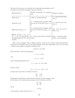
![4.24.2 1-dimensional representations
First, we describe the 1-dimensional representations of G.
Proposition 4.70. [G, G] = SL2(Fq).
Proof. Clearly,
det(xyx−1
y−1
) = 1,
so
[G, G] ⊆ SL2(Fq).
To show the converse, it suffices to show that the matrices
1 1
0 1
,
a 0
0 a−1 ,
1 0
1 1
are commutators (as such matrices generate SL2(Fq).) Clearly, by using transposition, it suffices
to show that only the first two matrices are commutators. But it is easy to see that the matrix
1 1
0 1
is the commutator of the matrices
A =
1 1/2
0 1
, B =
1 0
0 −1
,
while the matrix
a 0
0 a−1
is the commutator of the matrices
A =
a 0
0 1
, B =
0 1
1 0
,
This completes the proof.
Therefore,
G/[G, G] ∼= F×
q via g → det(g).
The one-dimensional representations of G thus have the form
ρ(g) = ξ det(g) ,
where ξ is a homomorphism
ξ : F×
q → C×
;
so there are q − 1 such representations, denoted Cξ.
70](https://image.slidesharecdn.com/replect-150306080251-conversion-gate01/85/Replect-70-320.jpg)
![4.24.3 Principal series representations
Let
B ⊂ G, B = {
∗ ∗
0 ∗
}
(the set of upper triangular matrices); then
|B| = (q − 1)2
q,
[B, B] = U = {
1 ∗
0 1
},
and
B/[B, B] ∼= F×
q × F×
q
(the isomorphism maps an element of B to its two diagonal entries).
Let
λ : B → C×
be a homomorphism defined by
λ
a b
0 c
= λ1(a)λ2(c),for some pair of homomorphisms λ1, λ2 : F×
q → C×
.
Define
Vλ1,λ2 = IndG
BCλ,
where Cλ is the 1-dimensional representation of B in which B acts by λ. We have
dim(Vλ1,λ2 ) =
|G|
|B|
= q + 1.
Theorem 4.71. 1. λ1 = λ2 ⇒ Vλ1,λ2 is irreducible.
2. λ1 = λ2 = µ ⇒ Vλ1,λ2 = Cµ ⊕ Wµ, where Wµ is a q-dimensional irreducible representation of
G.
3. Wµ
∼= Wν if and only if µ = ν; Vλ1,λ2
∼= Vλ′
1,λ′
2
if and only if {λ1, λ2} = {λ
′
1, λ
′
2} (in the
second case, λ1 = λ2, λ
′
1 = λ
′
2).
Proof. From the Mackey formula, we have
trVλ1,λ2
(g) =
1
|B|
a∈G, aga−1∈B
λ(aga−1
).
If
g =
x 0
0 x
,
the expression on the right evaluates to
λ(g)
|G|
|B|
= λ1(x)λ2(x) q + 1 .
If
g =
x 1
0 x
,
71](https://image.slidesharecdn.com/replect-150306080251-conversion-gate01/85/Replect-71-320.jpg)
![the expression evaluates to
λ(g) · 1,
since here
aga−1
∈ B ⇒ a ∈ B.
If
g =
x 0
0 y
,
the expression evaluates to
λ1(x)λ2(y) + λ1(y)λ2(x) · 1,
since here
aga−1
∈ B ⇒ a ∈ B or a is an element of B multiplied by the transposition matrix.
If
g =
x εy
y x
, x = y
the expression on the right evaluates to 0 because matrices of this type don’t have eigenvalues over
Fq (and thus cannot be conjugated into B). From the definition, λi(x)(i = 1, 2) is a root of unity,
so
|G| χVλ1,λ2
, χVλ1,λ2
= (q + 1)2
(q − 1) + (q2
− 1)(q − 1)
+ 2(q2
+ q)
(q − 1)(q − 2)
2
+ (q2
+ q)
x=y
λ1(x)λ2(y)λ1(y)λ2(x).
The last two summands come from the expansion
|a + b|2
= |a|2
+ |b|2
+ ab + ab.
If
λ1 = λ2 = µ,
the last term is equal to
(q2
+ q)(q − 2)(q − 1),
and the total in this case is
(q + 1)(q − 1)[(q + 1) + (q − 1) + 2q(q − 2)] = (q + 1)(q − 1)2q(q − 1) = 2|G|,
so
χVλ1,λ2
, χVλ1,λ2
= 2.
Clearly,
Cµ ⊆ IndG
BCµ,µ,
since
HomG(Cµ, IndG
BCµ,µ) = HomB(Cµ, Cµ) = C (Theorem 4.33).
Therefore, IndG
BCµ,µ = Cµ ⊕ Wµ; Wµ is irreducible; and the character of Wµ is different for distinct
values of µ, proving that Wµ are distinct.
72](https://image.slidesharecdn.com/replect-150306080251-conversion-gate01/85/Replect-72-320.jpg)
![If λ1 = λ2, let z = xy−1, then the last term of the summation is
(q2
+ q)
x=y
λ1(z)λ2(z) = (q2
+ q)
x;z=1
λ1
λ2
(z) = (q2
+ q)(q − 1)
z=1
λ1
λ2
(z).
Since
z∈F×
q
λ1
λ2
(z) = 0,
because the sum of all roots of unity of a given order m > 1 is zero, the last term becomes
−(q2
+ q)(q − 1)
z=1
λ1
λ2
(1) = −(q2
+ q)(q − 1).
The difference between this case and the case of λ1 = λ2 is equal to
−(q2
+ q)[(q − 2)(q − 1) + (q − 1)] = |G|,
so this is an irreducible representation by Lemma 4.27.
To prove the third assertion of the theorem, we look at the characters on hyperbolic elements
and note that the function
λ1(x)λ2(y) + λ1(y)λ2(x)
determines λ1, λ2 up to permutation.
4.24.4 Complementary series representations
Let Fq2 ⊃ Fq be a quadratic extension Fq(
√
ε), ε ∈ Fq F2
q. We regard this as a 2-dimensional vector
space over Fq; then G is the group of linear transformations of Fq2 over Fq. Let K ⊂ G be the cyclic
group of multiplications by elements of F×
q2 ,
K = {
x εy
y x
}, |K| = q2
− 1.
For ν : K → C× a homomorphism, let
Yν = IndG
KCν.
This representation, of course, is very reducible. Let us compute its character, using the Mackey
formula. We get
χ
x 0
0 x
= q(q − 1)ν(x);
χ(A) = 0 for A parabolic or hyperbolic;
χ
x εy
y x
= ν
x εy
y x
+ ν
x εy
y x
q
.
The last assertion holds because if we regard the matrix as an element of Fq2 , conjugation is an
automorphism of Fq2 over Fq, but the only nontrivial automorphism of Fq2 over Fq is the qth power
map.
73](https://image.slidesharecdn.com/replect-150306080251-conversion-gate01/85/Replect-73-320.jpg)
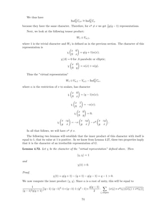
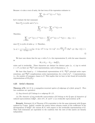
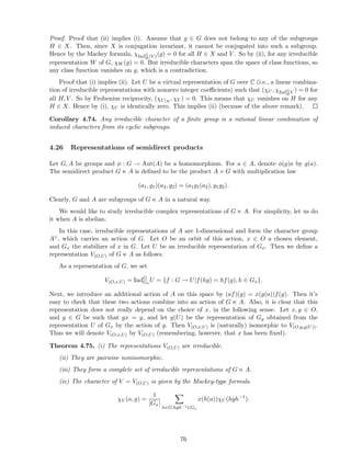
![5 Quiver Representations
5.1 Problems
Problem 5.1. Field embeddings. Recall that k(y1, ..., ym) denotes the field of rational functions
of y1, ..., ym over a field k. Let f : k[x1, ..., xn] → k(y1, ..., ym) be an injective k-algebra homomor-
phism. Show that m ≥ n. (Look at the growth of dimensions of the spaces WN of polynomials of
degree N in xi and their images under f as N → ∞). Deduce that if f : k(x1, ..., xn) → k(y1, ..., ym)
is a field embedding, then m ≥ n.
Problem 5.2. Some algebraic geometry.
Let k be an algebraically closed field, and G = GLn(k). Let V be a polynomial representation
of G. Show that if G has finitely many orbits on V then dim(V ) ≤ n2. Namely:
(a) Let x1, ..., xN be linear coordinates on V . Let us say that a subset X of V is Zariski dense
if any polynomial f(x1, ..., xN ) which vanishes on X is zero (coefficientwise). Show that if G has
finitely many orbits on V then G has at least one Zariski dense orbit on V .
(b) Use (a) to construct a field embedding k(x1, ..., xN ) → k(gpq), then use Problem 5.1.
(c) generalize the result of this problem to the case when G = GLn1 (k) × ... × GLnm (k).
Problem 5.3. Dynkin diagrams.
Let Γ be a graph, i.e., a finite set of points (vertices) connected with a certain number of edges
(we allow multiple edges). We assume that Γ is connected (any vertex can be connected to any
other by a path of edges) and has no self-loops (edges from a vertex to itself). Suppose the vertices
of Γ are labeled by integers 1, ..., N. Then one can assign to Γ an N × N matrix RΓ = (rij), where
rij is the number of edges connecting vertices i and j. This matrix is obviously symmetric, and is
called the adjacency matrix. Define the matrix AΓ = 2I − RΓ, where I is the identity matrix.
Main definition: Γ is said to be a Dynkin diagram if the quadratic from on RN with matrix
AΓ is positive definite.
Dynkin diagrams appear in many areas of mathematics (singularity theory, Lie algebras, rep-
resentation theory, algebraic geometry, mathematical physics, etc.) In this problem you will get a
complete classification of Dynkin diagrams. Namely, you will prove
Theorem. Γ is a Dynkin diagram if and only if it is one on the following graphs:
• An : ◦−−◦ · · · ◦−−◦
• Dn:
◦−−◦ · · · ◦−−◦
|
◦
• E6 : ◦−−◦−−◦−−◦−−◦
|
◦
78](https://image.slidesharecdn.com/replect-150306080251-conversion-gate01/85/Replect-78-320.jpg)
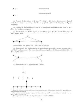
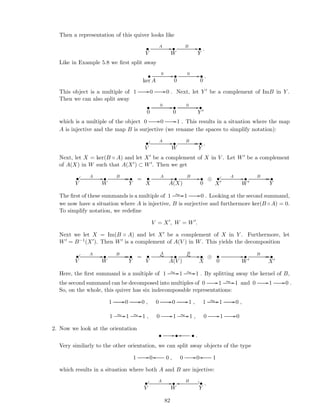
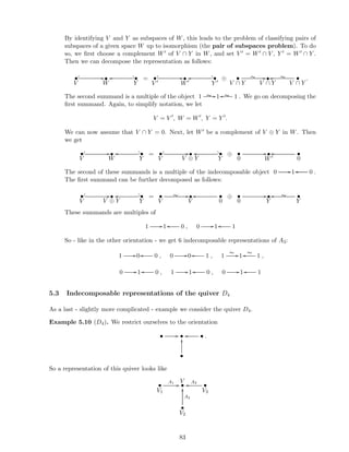
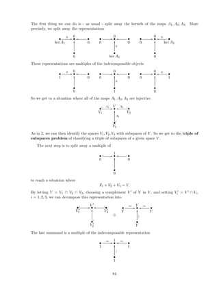
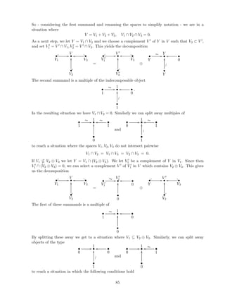
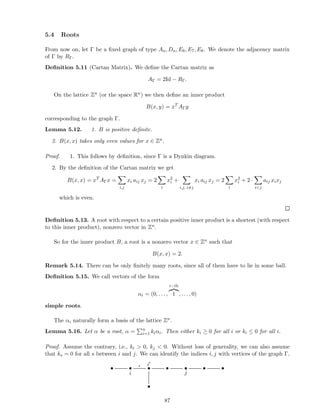
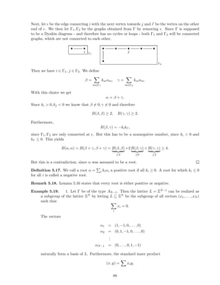
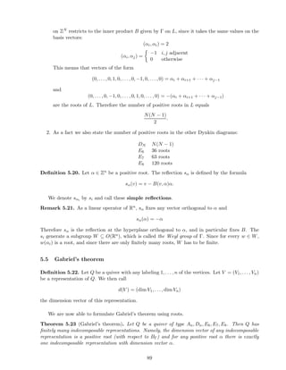
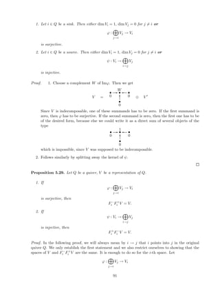
![6 Introduction to categories
6.1 The definition of a category
We have now seen many examples of representation theories and of operations with representations
(direct sum, tensor product, induction, restriction, reflection functors, etc.) A context in which one
can systematically talk about this is provided by Category Theory.
Category theory was founded by Saunders MacLane and Samuel Eilenberg around 1940. It is a
fairly abstract theory which seemingly has no content, for which reason it was christened “abstract
nonsense”. Nevertheless, it is a very flexible and powerful language, which has become totally
indispensable in many areas of mathematics, such as algebraic geometry, topology, representation
theory, and many others.
We will now give a very short introduction to Category theory, highlighting its relevance to the
topics in representation theory we have discussed. For a serious acquaintance with category theory,
the reader should use the classical book [McL].
Definition 6.1. A category C is the following data:
(i) a class of objects Ob(C);
(ii) for every objects X, Y ∈ Ob(C), the class HomC(X, Y ) = Hom(X, Y ) of morphisms (or
arrows) from X, Y (for f ∈ Hom(X, Y ), one may write f : X → Y );
(iii) For any objects X, Y, Z ∈ Ob(C), a composition map Hom(Y, Z)×Hom(X, Y ) → Hom(X, Z),
(f, g) → f ◦ g,
which satisfy the following axioms:
1. The composition is associative, i.e., (f ◦ g) ◦ h = f ◦ (g ◦ h);
2. For each X ∈ Ob(C), there is a morphism 1X ∈ Hom(X, X), called the unit morphism, such
that 1X ◦ f = f and g ◦ 1X = g for any f, g for which compositions make sense.
Remark. We will write X ∈ C instead of X ∈ Ob(C).
Example 6.2. 1. The category Sets of sets (morphisms are arbitrary maps).
2. The categories Groups, Rings (morphisms are homomorphisms).
3. The category Vectk of vector spaces over a field k (morphisms are linear maps).
4. The category Rep(A) of representations of an algebra A (morphisms are homomorphisms of
representations).
5. The category of topological spaces (morphisms are continuous maps).
6. The homotopy category of topological spaces (morphisms are homotopy classes of continuous
maps).
Important remark. Unfortunately, one cannot simplify this definition by replacing the word
“class” by the much more familiar word “set”. Indeed, this would rule out the important Example 1,
as it is well known that there is no set of all sets, and working with such a set leads to contradictions.
The precise definition of a class and the precise distinction between a class and a set is the subject
of set theory, and cannot be discussed here. Luckily, for most practical purposes (in particular, in
these notes), this distinction is not essential.
98](https://image.slidesharecdn.com/replect-150306080251-conversion-gate01/85/Replect-98-320.jpg)
![We also mention that in many examples, including examples 1-6, the word “class” in (ii) can
be replaced by “set”. Categories with this property (that Hom(X, Y ) is a set for any X, Y ) are
called locally small; many categories that we encounter are of this kind.
Sometimes the collection Hom(X, Y ) of morphisms from X to Y in a given locally small category
C is not just a set but has some additional structure (say, the structure of an abelian group, or
a vector space over some field). In this case one says that C is enriched over another category
D (which is a monoidal category, i.e., has a product operation and a neutral object under this
product, e.g. the category of abelian groups or vector spaces). This means that for each X, Y ∈ C,
Hom(X, Y ) is an object of D, and the composition Hom(Y, Z) × Hom(X, Y ) → Hom(X, Z) is a
morphism in D. For a more detailed discussion of this, we refer the reader to [McL].
Example. The category Rep(A) of representations of a k-algebra A is enriched over the
category of k-vector spaces.
Definition 6.3. A full subcategory of a category C is a category C′ whose objects are a subclass
of objects of C, and HomC′ (X, Y ) = HomC(X, Y ).
Example. The category AbelianGroups is a full subcategory of the category Groups.
6.2 Functors
We would like to define arrows between categories. Such arrows are called functors.
Definition 6.4. A functor F : C → D between categories C and D is
(i) a map F : Ob(C) → Ob(D);
(ii) for each X, Y ∈ C, a map F = FX,Y : Hom(X, Y ) → Hom(F(X), F(Y )) which preserves
compositions and identity morphisms.
Note that functors can be composed in an obvious way. Also, any category has the identity
functor.
Example 6.5. 1. A (locally small) category C with one object X is the same thing as a monoid.
A functor between such categories is a homomorphism of monoids.
2. Forgetful functors Groups → Sets, Rings → AbelianGroups.
3. The opposite category of a given category is the same category with the order of arrows and
compositions reversed. Then V → V ∗ is a functor Vectk → Vectop
k .
4. The Hom functors: If C is a locally small category then we have the functor C → Sets given
by Y → Hom(X, Y ) and Cop → Sets given by Y → Hom(Y, X).
5. The assignment X → Fun(X, Z) is a functor Sets → Ringsop
.
6. Let Q be a quiver. Consider the category C(Q) whose objects are the vertices and morphisms
are oriented paths between them. Then functors from C(Q) to Vectk are representations of Q over
k.
7. Let K ⊂ G be groups. Then we have the induction functor IndG
K : Rep(K) → Rep(G), and
ResG
K : Rep(G) → Rep(K).
8. We have an obvious notion of the Cartesian product of categories (obtained by taking the
Cartesian products of the classes of objects and morphisms of the factors). The functors of direct
99](https://image.slidesharecdn.com/replect-150306080251-conversion-gate01/85/Replect-99-320.jpg)
![Example 6.13. 1. Let V be a finite dimensional representation of a group G or a Lie algebra g.
Then the left and right adjoint to the functor V ⊗ on the category of representations of G is the
functor V ∗⊗.
2. The functor ResG
K is left adjoint to IndG
K. This is nothing but the statement of the Frobenius
reciprocity.
3. Let Assock be the category of associative unital algebras, and Liek the category of Lie
algebras over some field k. We have a functor L : Assock → Liek, which attaches to an associative
algebra the same space regarded as a Lie algebra, with bracket [a, b] = ab − ba. Then the functor L
has a left adjoint, which is the functor U of taking the universal enveloping algebra of a Lie algebra.
4. We have the functor GL1 : Assock → Groups, given by A → GL1(A) = A×. This functor
has a left adjoint, which is the functor G → k[G], the group algebra of G.
5. The left adjoint to the forgetful functor Assock → Vectk is the functor of tensor algebra:
V → TV . Also, if we denote by Commk the category of commutative algebras, then the left adjoint
to the forgetful functor Commk → Vectk is the functor of the symmetric algebra: V → SV .
One can give many more examples, spanning many fields. These examples show that adjoint
functors are ubiquitous in mathematics.
6.7 Abelian categories
The type of categories that most often appears in representation theory is abelian categories.
The standard definition of an abelian category is rather long, so we will not give it here, referring
the reader to the textbook [Fr]; rather, we will use as the definition what is really the statement of
the Freyd-Mitchell theorem:
Definition 6.14. An abelian category is a category (enriched over the category of abelian groups),
which is equivalent to a full subcategory C of the category A-mod of left modules over a ring A,
closed under taking finite direct sums, as well as kernels, cokernels, and images of morphisms.
We see from this definition that in an abelian category, Hom(X, Y ) is an abelian group for each
X, Y , compositions are group homomorphisms with respect to each argument, there is the zero ob-
ject, the notion of an injective morphism (monomorphism) and surjective morphism (epimorphism),
and every morphism has a kernel, a cokernel, and an image.
Example 6.15. The category of modules over an algebra A and the category of finite dimensional
modules over A are abelian categories.
Remark 6.16. The good thing about Definition 6.14 is that it allows us to visualize objects,
morphisms, kernels, and cokernels in terms of classical algebra. But the definition also has a big
drawback, which is that even if C is the whole category A-mod, the ring A is not determined by C.
In particular, two different rings can have equivalent categories of modules (such rings are called
Morita equivalent). Actually, it is worse than that: for many important abelian categories there
is no natural (or even manageable) ring A at all. This is why people prefer to use the standard
definition, which is free from this drawback, even though it is more abstract.
We say that an abelian category C is k-linear if the groups HomC(X, Y ) are equipped with
a structure of a vector space over k, and composition maps are k-linear in each argument. In
particular, the categories in Example 6.15 are k-linear.
103](https://image.slidesharecdn.com/replect-150306080251-conversion-gate01/85/Replect-103-320.jpg)
![7 Structure of finite dimensional algebras
In this section we return to studying the structure of finite dimensional algebras. Throughout the
section, we work over an algebraically closed field k (of any characteristic).
7.1 Projective modules
Let A be an algebra, and P be a left A-module.
Theorem 7.1. The following properties of P are equivalent:
(i) If α : M → N is a surjective morphism, and ν : P → N any morphism, then there exists a
morphism µ : P → M such that α ◦ µ = ν.
(ii) Any surjective morphism α : M → P splits, i.e., there exists µ : P → M such that α◦µ = id.
(iii) There exists another A-module Q such that P ⊕ Q is a free A-module, i.e., a direct sum of
copies of A.
(iv) The functor HomA(P, ?) on the category of A-modules is exact.
Proof. To prove that (i) implies (ii), take N = P. To prove that (ii) implies (iii), take M to be free
(this can always be done since any module is a quotient of a free module). To prove that (iii) implies
(iv), note that the functor HomA(P, ?) is exact if P is free (as HomA(A, N) = N), so the statement
follows, as if the direct sum of two complexes is exact, then each of them is exact. To prove that
(iv) implies (i), let K be the kernel of the map α, and apply the exact functor HomA(P, ?) to the
exact sequence
0 → K → M → N → 0.
Definition 7.2. A module satisfying any of the conditions (i)-(iv) of Theorem 7.1 is said to be
projective.
7.2 Lifting of idempotents
Let A be a ring, and I ⊂ A a nilpotent ideal.
Proposition 7.3. Let e0 ∈ A/I be an idempotent, i.e., e2
0 = e0. There exists an idempotent e ∈ A
which is a lift of e0 (i.e., it projects to e0 under the reduction modulo I). This idempotent is unique
up to conjugation by an element of 1 + I.
Proof. Let us first establish the statement in the case when I2 = 0. Note that in this case I is a
left and right module over A/I. Let e∗ be any lift of e0 to A. Then e2
∗ − e∗ = a ∈ I, and e0a = ae0.
We look for e in the form e = e∗ + b, b ∈ I. The equation for b is e0b + be0 − b = a.
Set b = (2e0 − 1)a. Then
e0b + be0 − b = 2e0a − (2e0 − 1)a = a,
so e is an idempotent. To classify other solutions, set e′ = e + c. For e′ to be an idempotent, we
must have ec + ce − c = 0. This is equivalent to saying that ece = 0 and (1 − e)c(1 − e) = 0, so
c = ec(1 − e) + (1 − e)ce = [e, [e, c]]. Hence e′ = (1 + [c, e])e(1 + [c, e])−1.
106](https://image.slidesharecdn.com/replect-150306080251-conversion-gate01/85/Replect-106-320.jpg)
![Now, in the general case, we prove by induction in k that there exists a lift ek of e0 to A/Ik+1,
and it is unique up to conjugation by an element of 1 + Ik (this is sufficient as I is nilpotent).
Assume it is true for k = m − 1, and let us prove it for k = m. So we have an idempotent
em−1 ∈ A/Im, and we have to lift it to A/Im+1. But (Im)2 = 0 in A/Im+1, so we are done.
Definition 7.4. A complete system of orthogonal idempotents in a unital algebra B is a collection
of elements e1, ..., en ∈ B such that eiej = δijei, and n
i=1 ei = 1.
Corollary 7.5. Let e01, ..., e0m be a complete system of orthogonal idempotents in A/I. Then there
exists a complete system of orthogonal idempotents e1, ..., em (eiej = δijei, ei = 1) in A which
lifts e01, ..., e0m.
Proof. The proof is by induction in m. For m = 2 this follows from Proposition 7.3. For m 2,
we lift e01 to e1 using Proposition 7.3, and then apply the induction assumption to the algebra
(1 − e1)A(1 − e1).
7.3 Projective covers
Obviously, every finitely generated projective module over a finite dimensional algebra A is a direct
sum of indecomposable projective modules, so to understand finitely generated projective modules
over A, it suffices to classify indecomposable ones.
Let A be a finite dimensional algebra, with simple modules M1, ..., Mn.
Theorem 7.6. (i) For each i = 1, ..., n there exists a unique indecomposable finitely generated
projective module Pi such that dim Hom(Pi, Mj) = δij.
(ii) A = ⊕n
i=1(dim Mi)Pi.
(iii) any indecomposable finitely generated projective module over A is isomorphic to Pi for
some i.
Proof. Recall that A/Rad(A) = ⊕n
i=1 End(Mi), and Rad(A) is a nilpotent ideal. Pick a basis of
Mi, and let e0
ij = Ei
jj, the rank 1 projectors projecting to the basis vectors of this basis (j =
1, ..., dim Mi). Then e0
ij are orthogonal idempotents in A/Rad(A). So by Corollary 7.5 we can lift
them to orthogonal idempotents eij in A. Now define Pij = Aeij. Then A = ⊕i ⊕dim Mi
j=1 Pij, so Pij
are projective. Also, we have Hom(Pij, Mk) = eijMk, so dim Hom(Pij, Mk) = δik. Finally, Pij is
independent of j up to an isomorphism, as eij for fixed i are conjugate under A× by Proposition
7.3; thus we will denote Pij by Pi.
We claim that Pi is indecomposable. Indeed, if Pi = Q1 ⊕ Q2, then Hom(Ql, Mj) = 0 for all j
either for l = 1 or for l = 2, so either Q1 = 0 or Q2 = 0.
Also, there can be no other indecomposable finitely generated projective modules, since any
such module has to occur in the decomposition of A. The theorem is proved.
References
[BGP] J. Bernstein, I. Gelfand, V. Ponomarev, Coxeter functors and Gabriel’s theorem, Russian
Math. Surveys 28 (1973), no. 2, 17–32.
107](https://image.slidesharecdn.com/replect-150306080251-conversion-gate01/85/Replect-107-320.jpg)
![[Cu] C. Curtis, Pioneers of Representation Theory: Frobenius, Burnside, Schur, and Brauer, AMS,
1999.
[CR] C. Curtis and I. Reiner, Representation Theory of Finite Groups and Associative Algebras,
AMS, 2006.
[FH] W. Fulton and J. Harris, Representation Theory, A first course, Springer, New York, 1991.
[Fr] Peter J. Freyd, Abelian Categories, an Introduction to the Theory of Functors. Harper and
Row (1964).
[McL] S. MacLane, Categories for a working Mathematician: 2nd Ed., Graduate Texts in Mathe-
matics 5, Springer, 1998.
108](https://image.slidesharecdn.com/replect-150306080251-conversion-gate01/85/Replect-108-320.jpg)

This document is an introduction to representation theory. It begins with basic notions such as what representation theory is, definitions of algebras, representations, ideals, quotients, and examples of algebras like quivers and Lie algebras. It then covers general results in representation theory, including representations of direct sums, filtrations, characters, and the Jordan-Holder and Krull-Schmidt theorems. Subsequent sections discuss representations of finite groups and quiver representations. The document concludes with an introduction to category theory concepts used in representation theory.