This document is a thesis that examines stochastic differential equations (SDEs). It begins with an introduction that provides background on SDEs and outlines the aims, objectives, and structure of the thesis. The body of the thesis first reviews key concepts in probability, Brownian motion, and stochastic integration. It then defines SDEs and explores numerical methods for solving SDEs such as the Euler-Maruyama and Milstein methods. Applications of SDEs in finance are also discussed, including the Black-Scholes option pricing model. The thesis concludes by summarizing the findings and proposing avenues for further research.


![2.2 Brownian Motion (or Wiener process)
This subsection provides the concept of Brownian Motion (or similarly Wiener Process)
and its properties as well as the proofs of them. Nowadays, it is known that Brownian
Motion is one of the most significant stochastic processes in Mathematics. Its name is
derived by the botanist Robert Brown, who observed by using a microscope the continuous
and irregular movement of particles in the water (at the age of 1827). The Brownian
process plays an important role in the theory of stochastic differential equations and
constitutes one of the cornerstones in mathematical finance and beyond.
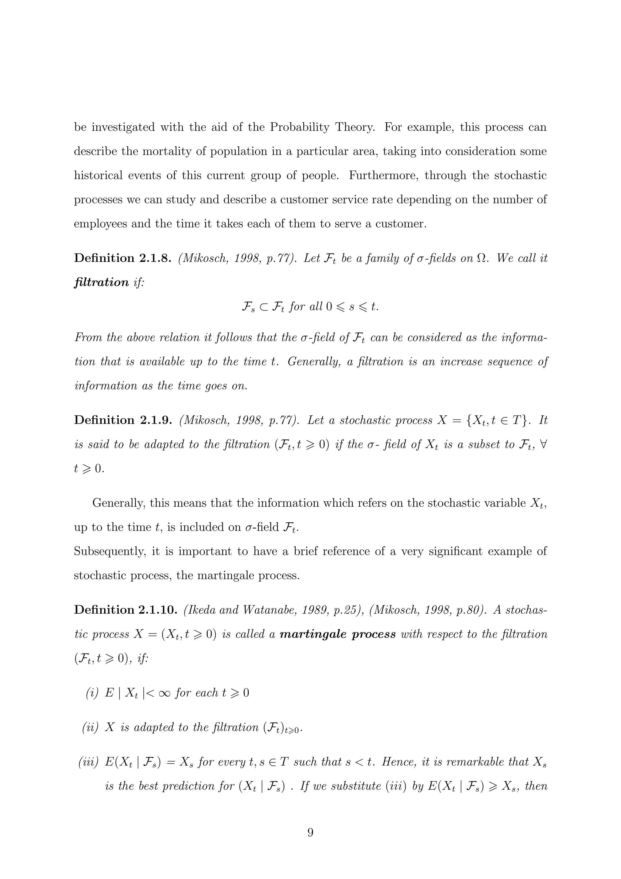
Figure 1: Two sample paths of standard Brownian motion on the time interval [0, 1] [see
code B.1.1].
Definition 2.2.1. Brownian Motion (or Wiener Process) (Friedman, 1975, p.36),
(Mikosch, 1998, p.33). Assume a stochastic process B = (Bt, t ∈ [0, ∞)). It is called
Brownian motion (or a Wiener process) if it satisfies the following conditions:
(i) B0 = x - this means that the process starts from the point x.
(ii) it has independent increments. For instance, for every sequence with 0 t1 < t2 <
. . . < tn, the increments:
Btn − Btn−1 , . . . , Bt2 − Bt1
are independent random variables.
11](https://image.slidesharecdn.com/b0d13018-fa0c-465f-86c0-5017f068511e-161113225724/75/final_report_template-14-2048.jpg)
![(iii) the increments Bt+h −Bt are normally distributed with expectation zero and variance
h.i.e.
Bt+h − Bt ∼ N(0, h)
(iv) Its sample paths are continuous.
Remark 2.2.2. (i) From Embrechts and Maejima(2000 p.6) and Mikosch(1998, p.33)
it can be seen that Brownian motion is closely linked to normal distribution.
(ii) Through the review of literature it is remarkable the fact that many definitions for
the Brownian motion assume that the process has 0 as a starting point. Specifically,
the condition (i) of the definition 2.2.1 is changed to B0 = 0, i.e. x = 0 and this
case is defined as a standard Brownian motion. Hence, the figure 1 (p. 7) shows
sample paths of standard Brownian motion. In this study it is determined any point
x to be a possible starting point of Brownian motion. (Mikosch, 1998, p.33), (Mao,
2007, p.15 ), (Friedman, 1975, p.36).
(iii) The condition (iv) of definition 2.2.1 can be found in many sources either as part of
the definition of Brownian motion, or as a property which follows from conditions
(i) − (iii). For instance on Mikosch(1998, p.33) it is written as a condition of the
definition. However, it is noticeable in the lecture presentation slides (Chapter 5,
p. 8/35) of Professor Philip O’Neill for the module of Stochastic Models that this
condition presents as a property of the Brownian motion. Furthermore, in Karatzas
and Shreve(1991, p.53-55) by using at first the Kolmogorov-Centsov Theorem and
then by considering the conditions (i)−(iii) of definition 2.2.1 to be the prerequisites
of the continuity, the desideratum is proved.
Corollary 2.2.3. Properties of Brownian Motion:
(i) 1. E[Bt | B0 = x] = x
2. V ar[Bt | B0 = x] = t
(ii) Sample paths of the Brownian motion are NOT differentiable.
12](https://image.slidesharecdn.com/b0d13018-fa0c-465f-86c0-5017f068511e-161113225724/75/final_report_template-15-2048.jpg)
![Proof. (i) From the condition (iii) we know that the probability density function is
f(x) = 1√
2πt
e
−x2
2t and the expectation of a general random variable g(Bt), where g
is a given function, is:
E[g(Bt)] =
1
√
2πt
∞
−∞
g(x)e
−x2
2t dx.
Using the above formula, it follows that:
E[Bt | B0 = x] = E[x + Bt] =
1
√
2πt
∞
−∞
(x + y)e
−y2
2t dy
. Therefore:
E[(x + Bt)] =
1
√
2πt
∞
−∞
(x + y)e
−y2
2t dy
=
1
√
2πt
∞
−∞
(xe
−y2
2t + ye
−y2
2t )dy
=
1
√
2πt
∞
−∞
(xe
−y2
2t )dy +
1
√
2πt
∞
−∞
(ye
−y2
2t )dy
=
x
√
2πt
∞
−∞
(e
−y2
2t )dy +
1
√
2πt
−te
−y2
2t
∞
−∞
=
x
√
2πt
∞
−∞
(e
−y2
2t )dy +
1
√
2πt
lim
y→∞
(−te
−y2
2t )
0
− lim
y→−∞
(−te
−y2
2t )
0
Set z =
y
√
2t
and dy = dz
√
2t.
=
x
√
2t
√
2πt
∞
−∞
e−z2
dz
√
π
=
x
√
2t
√
π
√
2πt
= x, as required.
13](https://image.slidesharecdn.com/b0d13018-fa0c-465f-86c0-5017f068511e-161113225724/75/final_report_template-16-2048.jpg)
![Whilst for the variance we have:
V ar[(x + Bt)] =
1
√
2πt
∞
−∞
(x + y)2
e
−y2
2t dy
=
x2
√
2πt
∞
−∞
e
−y2
2t dy +
2x
√
2πt
∞
−∞
(ye
−y2
2t )dy +
1
√
2πt
∞
−∞
y2
e
−y2
2t dy
=
1
√
2πt
y(−2te
−y2
2t )
∞
−∞
+
1
√
2πt
y(−te
−y2
2t )
∞
−∞
+
1
√
2πt
∞
−∞
y(−te
−y2
2t ) dy
= 0 + 0 −
1
√
2πt
∞
−∞
−te
−y2
2t dy
Set z =
y
√
2t
and dy = dz
√
2t.
=
t
√
2t
√
2πt
∞
−∞
e−z2
dz
√
π
= t, as required.
(ii) The basic consideration for this property is to show that Brownian motion is H-
self similar process defined in definition 2.2.5 below. That is the most important
point of the whole proof because we will subsequently show that any H-self similar
process is nowhere differentiable with probability 1. This particular syllogism can
lead us to our initial purpose. Namely, to show that Brownian motion is nowhere
differentiable. First of all, it is necessary to refer some helpful definitions.
Definition 2.2.4. (Mikosch, 1998, p.30). Let a stochastic process X = (Xt, t ∈ T)
and T be a subset of R. The process X has stationary increments if:
Xt − Xs
d
= Xt+h − Xs+h ∀t, s ∈ T and t + h, s + h ∈ T.
Definition 2.2.5. [Embrechts and Maejima, 2000, p.3] Assuming a stochastic pro-
cess X = (Xt, t = 0, 1, 2, 3, . . .). It is called to be ”H-self-similar” if ∀a > 0, ∃H > 0
such that:
{Xat}
d
= {aH
Xt}
In plain words, the term of ”self-similarity” can be described as the ability of a
graph which if you choose any part of it, in any time length interval, you can earn
the similar image as the initial one. It is important to note that you can’t get the
14](https://image.slidesharecdn.com/b0d13018-fa0c-465f-86c0-5017f068511e-161113225724/75/final_report_template-17-2048.jpg)
![same image as the original.
The following proposition is stated without proof in Mikosch(1998, p.36). A proof
of this result is given below.
Proposition 2.2.6. (Mikosch, 1998, p.36). Let {Bt, t 0} be a standard Brownian
Motion. Then {Bt} is 1
2
-self-similar process.
Proof. According to the proof of Embrechts and Maejima [2000, p. 5] it is obvious
that the proof which is given has brief description. As a result, in this thesis it is
provided a detailed proof to show that {Bt} is 1
2
-self-similar process.
From definition 2.2.4, we consider the relation below:
{Bat}
d
= {a
1
2 Bt} ∀a > 0.
However, it would be simpler to be proven that:
{a−1
2 Bat}
d
= {Bt} ∀a > 0.
Hence, we have to examine if the above relation can satisfy the conditions of the
definition 2.2.1. The condition (i) (of definition 2.2.1) is shown as below:
For t = 0,
{a−1
2 B0}
B0=0
= 0.
Moreover, to proof the condition (ii) (of definition 2.2.1), it is enough to show
that for all 0 t1 t2 . . . tk the random variables:
a−1
2 Bat1 − a−1
2 Bat0 , a−1
2 Bat2 − a−1
2 Bat1 , . . . , a−1
2 Batk
− a−1
2 Batk−1
have correlation equals to zero. Hence, when ti < tj:
E[(a−1
2 Bati
− a−1
2 Bati−1
)(a−1
2 Batj
− a−1
2 Batj−1
)] =
= E[a−1
Bati
Batj
− a−1
Bati
Batj−1
− a−1
Bati−1
Batj
+ a−1
Bati−1
Batj−1
]
= a−1
[ati − ati − ati−1 + ati−1] = 0
15](https://image.slidesharecdn.com/b0d13018-fa0c-465f-86c0-5017f068511e-161113225724/75/final_report_template-18-2048.jpg)
![and we conclude to the deduction that a−1
2 Bt has independent increments. Regards
the condition (iii) (of definition 2.2.1) we proceed with the following methods:
E[a−1
2 Bat] = a−1
2 E[Bat] = 0
E[(a−1
2 Bat)2
] = a−1
at = t
Finally, the condition (iv) follows from the condition (i) to (iii). Consequently
{a−1
2 Bat}
d
= {Bt} as required.
Figure 2: Self-similarity of Brownian motion (Mikosch, 1998, p.37).
16](https://image.slidesharecdn.com/b0d13018-fa0c-465f-86c0-5017f068511e-161113225724/75/final_report_template-19-2048.jpg)
![Thus, from the proportions 2.2.6 and 2.2.7 it follows that a Brownian sample path
is nowhere differentiable.
Therefore, we have just completed the proves of properties which were referred on
corollary 2.2.3.
Remark 2.2.8. As can be seen from Figure 1, which illustrates two random sample paths
of Brownian motion, it is noticeable that there is no regularity in the trend of the paths.
Therefore, the non-differentiability of Brownian motion is distinguishable by its graphical
representation.
Theorem 2.2.9. (Embrecht and Maejima, 2000, p.4). Let a stochastic process {Xt} be
H-self-similar and we assume E[X2
(1)] < ∞. Then
E[XtXs] =
1
2
{t2H
+ s2H
− |t − s|2H
}E[X2
1 ]
.
Proof.
E[X2
t ] = V ar[Xt] = V ar[tH
X1] = t2H
V ar[X1] = t2H
E[X2
1 ]
E[X2
s ] = V ar[Xs] = V ar[sH
X1] = s2H
V ar[X1] = s2H
E[X2
1 ]
E[(Xt − Xs)2
] = V ar[(Xt − Xs)] = V ar[X1(| t − s |)H
] =| t − s |2H
E[X2
1 ]
Therefore,
E[XtXs] =
1
2
{E[X2
t ] + E[X2
s ] − E[(Xt − Xs)2
]}
=
1
2
t2H
+ s2H
− |t − s|2H
E[X2
1 ]
Theorem 2.2.10. E[BtBs] = min {t, s}
18](https://image.slidesharecdn.com/b0d13018-fa0c-465f-86c0-5017f068511e-161113225724/75/final_report_template-21-2048.jpg)
![Proof. As we can see in Embrecht and Maejima(2000, p.5) the proof is based on the fact
that standard Brownian motion is 1
2
-self-similar process. Therefore, it can be used the
formula of the theorem 2.2.9. as below:
E[BtBs] =
1
2
t2H
+ s2H
− |t − s|2H
≡ min {t, s} .
Thus it helps us to acquire the desired result.
However, it can be provided in this thesis a second method in order to prove E[BtBs] =
min {t, s}.
Let assume 0 < t < s. Then,
Bs = Bs + Bt − Bt
BtBs = BtBs + B2
t − B2
t
BtBs = B2
t + Bt[Bs − Bt]
(linearity of expectation) E[BtBs] = E[B2
t ] + E[Bt[Bs − Bt]]
(by def.2.2.1, cond. (ii) and (iii)) E[BtBs] = t + 0 = t
Now, let assume 0 < s < t. Then,
Bt = Bt + Bs − Bs
BtBs = BtBs + B2
s − B2
s
BtBs = B2
s + Bs[Bt − Bs]
(linearity of expectation) E[BtBs] = E[B2
s ] + E[Bs[Bt − Bs]]
(by def.2.2.1, cond. (ii) and (iii)) E[BtBs] = s + 0 = s
Therefore, it is proved that E[BtBs] = min {t, s}.
Example 2.2.11. Find E[(Bt+w − Bt)2
] for t, w > 0.
E[(Bt+w − Bt)2
] = E[B2
t+w − 2BtBt+w + B2
t ]
(linearity of expectation) = E[B2
t+w] − 2E[BtBt+w] + E[B2
t ]
(by def.2.2.1, cond. (ii)(iii) and theorem 2.2.10) = t + w − 2t + t
= w.
19](https://image.slidesharecdn.com/b0d13018-fa0c-465f-86c0-5017f068511e-161113225724/75/final_report_template-22-2048.jpg)
![The above example shows that E[(dBt)2
] = dt where dBt = Bt+w −Bt. Specifically, the
expectation of (dBt)2
equals to the difference of t+dt and t. Obviously, V ar[Bt+w −Bt] =
E[(Bt+w − Bt)2
] since E[Bt+w − Bt] = 0.
2.3 Brief mention to Stieltjes integral
In this subsection we give a brief mention to the concept of Stieltjes integral and explain
why this concept is not valid for the definition of a stochastic integral. Initially, we start
by the definition of the Stieltjes integral for a step function.
Definition 2.3.1. (Dragomir, 2001, p.42). Consider a step function:
h = h010 +
n
i=1
h01(ti,ti+1]
where {ti} is a partition of the interval [0, t]. Let m be a random function on R+
. The
Stieltjes integral of h over m is defined as below:
t
0
hdm :=
n
i=1
hi[m(ti+1) − m(ti)]
A continues function h can be approached by a sequence hn of step functions with the
concept that hn → h. By this sequence we can create a new sequence consists by Stieltjes
integrals
t
0
hndm. Each one of these Stieltjes integrals is defined by the definition 2.3.1.
The limit, as n → ∞, exists and, actually, if hn and hn are two different sequences of
step functions which approach the same function h then the limits
t
0
hmdm and
t
0
hndm
coincide between each other. Consequently,
Definition 2.3.2. Consider h is a continues function and hn is a sequence of step func-
tions which approaches h. The Stieltjes integral of h over a function m is defined to
be:
t
0
h · dm := lim
n→∞
hn · dm
The function m is called integrator.
20](https://image.slidesharecdn.com/b0d13018-fa0c-465f-86c0-5017f068511e-161113225724/75/final_report_template-23-2048.jpg)
![The following theorem shows us the significance of the total variation of an integrator
in the Stieltjes integral. The proof is omitted since it is provided in many literatures e.g.
Dragomir(2001).
Theorem 2.3.3. Suppose m has a local bounded variation and h is continues function.
Then the Stieltjes integral
t
0
hdm exists and satisfies the condition:
|
t
0
hdm |
t
0
| h || dm | sup
0 s t
h(s)
t
0
| dm |
where
t
0
| dm |:= sup{
n
i=1
| m(ti+1) − m(ti) |}
and {ti} a possible partition of [0, t]. The supremum is obtained on all partitions.
The above theorem shows us that if an integrator does not have a finite variation then
the Stieltje’s integral has difficulties to be defined.
Consider now that the functions h and m are stochastic processes, i.e. h = h(t, w) and
m = m(t, w). Furthermore we define m(t, w) = Bt i.e. the integrator will be a Brownian
motion. The theorem (2.3.3) presents the main reason why a Stieltjes integral can not
exists with a Brownian motion as an integrator. A Brownian motion is a function with
an unbounded variation. Consequently, this specific characteristic puts forward the view
that the Steltjies integral can not be defined in terms of a Brownian motion, since the
integrator must be a bounded function. Therefore, the Steltjies integral can not define
stochastic integrals. The significant step to solve this problem is to set a limit as n → ∞
in L2
. This change in the determination of limit is the vital difference between the Itˆo’s
integral and Stieltjes integral.
2.4 Itˆo’s integral
As we have seen in a previous subsection the Brownian motion is a function which is
nowhere differentiable. However, the integration process can be applied to it. Hence,
through this subsection we will attend to the integration of a stochastic process with
21](https://image.slidesharecdn.com/b0d13018-fa0c-465f-86c0-5017f068511e-161113225724/75/final_report_template-24-2048.jpg)
![Brownian motion as an integrator. During the second world war, the Japanese math-
ematician Kyoshi Itˆo indicated the way to define this kind of integral and thus, it was
called the Itˆo’s stochastic integral. Today, this kind of integrations have applications in
many scientific fields, such as in Finance, Physics etc. Furthermore, on this subsection we
will see that the variation of Brownian motion is the main idea regarding the definition of
the Itˆo’s integral. Initially, we define the stochastic integral for stochastic step functions
and then, for ”suitable” stochastic processes.
Definition 2.4.1. A stochastic process f(t), t ∈ [a, b] is called a step function if there is
a finite sequence of numbers a = t0 < t1 < . . . < tn = b and a finite sequence of random
variables f0, f1, f2, . . . , fn−1 such that:
f(t) = fj if t ∈ (tj, tj+1], j = 1, 2, . . . , n − 1
Moreover, this kind of stochastic process f(t) can be written in form:
f(t) =
n−1
j=0
fj1(tj,tj+1](t) = f01[t0,t1](t) +
n−1
j=1
fj1(tj,tj+1](t) (2.3)
where,
1(tj,tj+1](t) =
0, if t ∈ (tj, tj+1]
1, if t ∈ (tj, tj+1].
From now on, we will denote the set of step functions on [a, b] as Mstep([a, b]).
From the above definition it is important to be mentioned the fact that the indicator
function is the reason of the appearance of steps in the graph of a step function.
2.4.1 The Itˆo’s integral for a step function
Then, it is defined the Itˆo’s stochastic integral for a step function.
Definition 2.4.2. The Itˆo’s integral for a step function Let a stochastic step func-
tion f of the form (2.3). The Itˆo’s integral of f in [a, b] with respect to the Brownian
22](https://image.slidesharecdn.com/b0d13018-fa0c-465f-86c0-5017f068511e-161113225724/75/final_report_template-25-2048.jpg)
![motion is defined as below:
I(f(t)) =
b
a
f(t)dBt =
n−1
j=0
fj(Btj+1
− Btj
).
Theorem 2.4.3. The Itˆo’s stochastic integral of a step function has the following prop-
erties:
(i) The Itˆo’s integral is linear, i.e. if f(t) and g(t) are two step functions then:
I(λ1f(t) + λ2g(t)) = λ1I(f(t)) + λ2I(g(t))
(ii)
E[I(f(t))] = E
b
a
f(t)dBt = 0
(iii) This property is called ”Itˆo’s isometry”:
E[I(f(t))]2
= E
b
a
f(t)dBt
2
=
b
a
E[f(t)]2
dt
Proof. (i) In Mao(2007, p.20), Allen(2007, p.70) and Mikosch(1998, p.107) the proof
leaves to the reader. However, the current thesis includes this proof as below:
I(λ1f(t) + λ2g(t)) =
b
a
(λ1f(t) + λ2g(t))dBt
by def. 2.4.2
=
n−1
j=0
(λ1fj + λ2gj)(Btj+1
− Btj
)
=
n−1
j=0
λ1fj(Btj+1
− Btj
) +
n−1
j=0
λ2gj(Btj+1
− Btj
)
= λ1
n−1
j=0
fj(Btj+1
− Btj
) + λ2
n−1
j=0
gj(Btj+1
− Btj
)
= λ1
b
a
f(t)dBt + λ2
b
a
g(t)dBt = λ1I(f(t)) + λ2I(g(t))
23](https://image.slidesharecdn.com/b0d13018-fa0c-465f-86c0-5017f068511e-161113225724/75/final_report_template-26-2048.jpg)
![(ii) By the definition 2.4.2:
E[I(f(t))] = E
b
a
f(t)dBt = E
n−1
i=0
fi(Bti+1
− Bti
)
=
n−1
i=0
E fi(Bti+1
− Bti
)
*
=
n−1
i=0
E[fi]E[Bti+1
− Bti
]
by def. 2.2.1
= 0.
explanetion of (*):
As we know, the variation Bti+1
− Bti
of Brownian motion is independent of Fti
.
Also, due to the fact that the random variable fi is Fti
− measurable, we conclude
that fi and Bti+1
− Bti
are independent.
(iii) According to some references, this proof is presented without detailed explanation.
Therefore this thesis provides a detailed step by step proof in order to have better
understanding and supervision of the methods that are used. Let assume a step
function f(t) of the form (2.3). Therefore, by the definition 2.4.2, this function has
the following stochastic integral:
I(f(t)) =
n−1
j=0
fj(Btj+1
− Btj
)
Then, it is able to be calculated the expectation of the square of the above quantity.
Indeed, by separating the diagonal and non-diagonal terms of the sum we get:
| I(f(t)) |2
=
n−1
j=0
f2
j (Btj+1
− Btj
)2
+ 2
k<j
fj(Btj+1
− Btj
)fk(Btk+1
− Btk
)
The variation of the Brownian motion (Btj+1
− Btj
) is independent of anything that
happened before of the time tj. Since the random variable fj is Ftj
measurable, the
random variables (Btj+1
− Btj
) and fj are independent. In addition, any function of
these variables have the same condition. Hence:
n−1
j=0
E[f2
j (Btj+1
− Btj
)2
] =
n−1
j=0
E[f2
j ]E[(Btj+1
− Btj
)2
] =
n−1
j=0
E[f2
j ](tj+1 − tj)
24](https://image.slidesharecdn.com/b0d13018-fa0c-465f-86c0-5017f068511e-161113225724/75/final_report_template-27-2048.jpg)
![since E[(Btj+1
− Btj
)2
] = (tj+1 − tj) (similar case and steps as the example 2.2.11).
Moreover, the random variables tk, Bt+1 −Btk
, tj, Bj+1 −Btj
are mutually indepen-
dent since j < k. Therefore:
E[fj(Btj+1
− Btj
)fk(Btk+1
− Btk
)] = 0
since E[Btj+1
− Btj
] = 0 by the conditions of the Brownian motion. By applying
the above steps it follows that:
E[I(f(t))]2
=
n−1
j=0
E[f2
j ](tj+1 − tj)
Afterwords, we proceed to the following step:
| f(t) |2
=
n−1
j=0
f2
j 1[tj,tj+1)(t) +
k<j
fkfj1[tj,tj+1)(t)1[tk,tk+1)(t) =
n−1
j=0
f2
j 1[tj,tj+1)(t)
since 1[tj,tj+1)(t)1[tk,tk+1)(t) = 0 for k < j. Then, following the previous steps we
have that:
E
b
a
| f(t) |2
dt
(2.3)
= E
b
a
|
n−1
j=0
fj1[tj,tj+1) |2
dt
=
n−1
j=0
E[f2
j ]
b
a
1[tj,tj+1)dt
=
n−1
j=0
E[f2
j ](tj+1 − tj).
Consequently the Itˆo Isometry is proved (Mao, 2007, p.19), (Øksendal, 2003, p.29).
Example 2.4.4. Let assume {Bt : t 0} to be a standard Brownian motion i.e.B0 = 0.
Calculate the expectation and the standard deviation of
∞
0
e−t
dBt.
Firstly, we are going to find the expectation.
E[
∞
0
e−t
dBt] = E[Itˆo] = 0.
25](https://image.slidesharecdn.com/b0d13018-fa0c-465f-86c0-5017f068511e-161113225724/75/final_report_template-28-2048.jpg)
![We know for the variance that:
V ar[X] = E[X2
] − E[X]2
.
Since E[Itˆo] = 0 then:
V ar[
∞
0
e−t
dBt] = E[(
∞
0
e−t
bBt)2
]
= E[(
∞
0
e−t
dBt)(
∞
0
e−t
dBt)]
(Itˆo’s isometry)
= E[
∞
0
e−2t
dt] =
1
−2e2t
∞
0
=
1
2
Finally the standard deviation is equals to 1√
2
.
Subsequently, it will be defined now a more general class of stochastic processes (not
necessarily only for step functions) for which we will be able to define the Itˆo’s stochastic
integral.
Definition 2.4.5. A stochastic process f(t) belongs to the set M2
([a, b]) if it is adapted
to the filtration Fs = σ(Bs, s t) and also it satisfies the condition:
E
b
a
| f(t) |2
dt < ∞
The stochastic processes that belongs to M2
([a, b]) can be approached by step functions
as this conclusion is demonstrated by the theorem below:
Theorem 2.4.6. For any f ∈ M2
([a, b]), there is a step function sequence fstep,n(t), such
that:
lim
n→∞
E
b
a
| f(t) − fstep,n(t) |2
dt = 0
i.e. the stochastic process f is the limit of fstep,n(t).
Proof. In this proof we follow the three steps according to Mao(2007, p.20) but with more
detailed assumptions. Before starting it is considered necessary to have a short reference
to the three steps of this proof and the main idea of using them. This reference will be
helpful for the reader to understand better the syllogism of this proof and to be adapted
26](https://image.slidesharecdn.com/b0d13018-fa0c-465f-86c0-5017f068511e-161113225724/75/final_report_template-29-2048.jpg)
![to its particularities.
The first step shows that any stochastic process which belongs to M2
([a, b]) can be
approached by a sequence of bounded processes in M2
([a, b]). The second step refers to
the fact that any bounded stochastic process in M2
([a, b]) can be approached by a sequence
which consists of bounded and continuous processes in M2
([a, b]). Consequently,
any stochastic process in M2
([a, b]) can be approached by a sequence of bounded and
continuous processes in M2
([a, b]). Finally, the third step demonstrates that any bounded
and continuous processes in M2
([a, b]) can be approached by a step function sequence.
The composition of these three steps concludes that any stochastic process which belongs
to M2
([a, b]) can be approached by a step function sequence. Then, we are ready to cite
the three steps analytically.
1st
step: Let the stochastic process f(t) ∈ M2
([a, b]). We define a sequence of stochastic
processes which is: φn(t) = [−n ∨ f(t)] ∧ n. The sequence φn(t) is bounded by f(t)
and so it belongs to M2
([a, b]) for every n. Furthermore,
f(t) = lim
n→∞
φn(t),
and by the dominated convergence theorem [see A.1] it follows:
E
b
a
lim
n→∞
| f(t) − φn(t) |2
dt = 0
2nd
step: Assume φ(t) ∈ M2
([a, b]) to be bounded and we are going to create a sequence ψn(t)
as follows: ∀n there is a continuous function ρn : R → R+
such that ρn(t) = 0 for
0 t 1
n
and
∞
−∞
ρn(t)dt = 1. Therefore, it feasible that:
ψn(t) =
b
a
ρn(s − t)φ(s)dt. (2.4)
It is remarkable the fact that ψn(t) is a sequence of stochastic processes because φ(s)
is a stochastic sequence too. The integral (2.4) is a Riemann-Stieltjes integral and by
its properties and the fact that ψ(t) is bounded we conclude that the sequence ψn(t) is
27](https://image.slidesharecdn.com/b0d13018-fa0c-465f-86c0-5017f068511e-161113225724/75/final_report_template-30-2048.jpg)
![consisted by continuous functions and ψ(t) is a bounded sequence. Since ψ(t) ∈ M2
([a, b])
and from the bounded convergence theorem [see A.2] it follows:
E
b
a
lim
n→∞
| f(t) − φn(t) |2
dt = 0
3rd
step: Finally, if ψ(t) ∈ M2
([a, b]) is bounded and continuous we can create the step
function sequence fstep,n as below:
fstep,n(t) = ψ(a)1[a,a+b−a
a
](t) +
n−1
i=1
ψ a + i
b − a
a
1(a+i b−a
a
,a+(i+1)b−a
a
](t)
The above sequence is bounded. By applying again the bounded convergence theorem
[see A.2] it concludes that:
lim
n→∞
E
b
a
| ψ(t) − fstep,n(t) |2
dt = 0
By the above three steps and the use of the triangle inequality we have the final result:
lim
n→∞
E
b
a
| f(t) − fstep,n(t) |2
dt = 0.
Example 2.4.7. Let’s wonder which will be the choice of the partition tj. One example
of such a choice is given below. Assume the initial interval [0, T]. One possible choice of a
partition that belongs to this interval would be: 0 = tn
0 < tn
1 < tn
2 < . . . < tn
j < . . . < tn
n =
T, where j = 0, . . . , n and tn
j = jT
n
. By using this partition it would be possible to choose
a sequence of step functions as the possible approach of the stochastic process f(t, ω) to
the interval [0, T]. This sequence would be:
fstep,n(t) =
n−1
j=0
f(tj, ω)1[tj,tj+1)(t).
If the stochastic process f(t, ω) is continuous with respect to the variable t, it follows that:
lim
n→∞
E
b
a
| f(t) − fstep,n(t) |2
dt = 0.
Namely, the sequence of step functions fstep,n approaches the stochastic process f. For
instance, let f(t, ω) = B2
t . An approximation of the stochastic process f is:
fstep,n(t) =
n−1
j=0
B2
jT
n
1[jT
n
,
(j+1)T
n
)
(t).
28](https://image.slidesharecdn.com/b0d13018-fa0c-465f-86c0-5017f068511e-161113225724/75/final_report_template-31-2048.jpg)
![2.4.2 C’s stochastic integral
As we have seen, any stochastic process f ∈ M2
([a, b]) can be approached by a sequence of
step functions fstep,n. Moreover, due to the fact that the stochastic integral is also defined
with respect to a stochastic step function, we are ready to define the Itˆo’s stochastic
integral as below:
Definition 2.4.8. Let f ∈ M2
([a, b]). The Itˆo’s integral of stochastic process f with
respect to Brownian motion is defined by the following limit:
I(f(t)) =
b
a
f(t)dBt := lim
n→∞
I(fstep,n(t)) = lim
n→∞
b
a
fstep,n(t)dBt
where
lim
n→∞
E |
b
a
f(t) − fstep,n(t)dBt |2
= 0.
As we can see, the I(f(t)) =
b
a
f(t)dBt is a random variable and it is the L2
limit of
the sequence of random variables I(fstep,n(t)) = limn→∞
b
a
fstep,n(t)dBt. i.e.
lim
n→∞
E | I(f(t)) − I(fstep,n(t)) |2
= 0.
The existence of the above definition is ensured by the convergence of I(fstep,n(t)) =
b
a
fstep,n(t)dBt in L2
(Ω, F, P). Hence, we conclude to the following theorem:
Theorem 2.4.9. Let f ∈ M2
([a, b]) and fstep,n(t) a step function sequence which ap-
proaches the process f(t). Therefore, the sequence of stochastic integrals I(fstep,n(t)) =
b
a
fstep,n(t)dBt goes to a square integrable random variable.i.e. tends to L2
(Ω, F, P).
Proof. Because of the completeness of L2
, it is enough to show that the sequence sn :=
I(fstep,n(t)) is a Cauchy sequence in L2
. i.e. sn − sm L2 → 0 for n, m → ∞. Indeed:
29](https://image.slidesharecdn.com/b0d13018-fa0c-465f-86c0-5017f068511e-161113225724/75/final_report_template-32-2048.jpg)
![sn − sm L2 := E | sn − sm |2
1
2
= E |
b
a
fstep,n(t)dBt −
b
a
fstep,m(t)dBt |2
1
2
(Theorm 2.4.3, (i))
= E |
b
a
fstep,n(t) − fstep,m(t)(t)dBt |2
1
2
(Itˆo’s isometry)
= E
b
a
| fstep,n(t) − fstep,m(t) |2
dt
1
2
= E
b
a
| fstep,n(t) − f(t) + f(t) − fstep,m(t) |2
dt
1
2
= fstep,n(t) − f(t) + f(t) − fstep,m(t) M2
fstep,n(t) − f(t) M2 + f(t) − fstep,m(t) M2 → 0 for n, m → ∞
because fstep,n(t) → f(t). For that reason, the limit of I(fstep,n(t)) exists in L2
(Ω, F, P)
and it is called I(f(t)). That is followed because of the completeness of L2
(Ω, F, P).
Hence, through the definition of the stochastic integral I(f(t)) we achieve to overcome
the main issue of the infinite variation of Brownian motion. We exploit the result that its
quadratic variation is bounded.
Corollary 2.4.10. ∀ f, g ∈ M2
([0, T]) applied that:
E[I(f(t))I(g(t))] = E
b
a
f(t)dBt ·
b
a
g(t)dBt = E
b
a
f(t)g(t)dt
Proof. We use the following formula:
ab =
1
4
(| a + b |)2
− | a − b |)2
(2.5)
where a = I(f) and b = I(g). By taking expectations and substituting a and b to (2.5) it
follows:
E[I(f)I(g)] =
1
4
(E[| I(f)+I(g) |2
]−E[| I(f)−I(g) |2
]) =
1
4
(E[| I(f+g) |2
]−E[| I(f−g) |2
])
(2.6)
30](https://image.slidesharecdn.com/b0d13018-fa0c-465f-86c0-5017f068511e-161113225724/75/final_report_template-33-2048.jpg)
![where it has been used the linearity of Itˆo’s stochastic integral. However from Itˆo’s
isometry,
E | I(f + g) |2
= E
T
0
| f + g |2
dt
E | I(f − g) |2
= E
T
0
| f − g |2
dt .
Thus,
E[I(f(t))I(g(t))] =
1
4
E
T
0
| f + g |2
dt − E
T
0
| f − g |2
dt
=
1
4
E
T
0
| f + g |2
− | f − g |2
dt
=
1
4
E
T
0
4fgdt = E
T
0
fgdt
The above proof is presented in different versions by Karatzas and Shreve(1991, p.180)
and Mao(2007, p.27).
An example to show the way which a stochastic integral is solved by its definition is now
given. This particular example is solved by Øksendal(2003, p.29) who uses the hypothesis
B0 = 0. However, in this thesis will be provided a more analytical proof without the
above assumption.
Example 2.4.11. According to the definition of Itˆo’s stochastic integral prove that:
I(Bt) =
T
0
BtdBt =
1
2
B2
T −
T
2
.
The integrable stochastic process is f(t, ω) = Bt. We choose the partition 0 = tn
0 < tn
1 <
tn
2 < . . . < tn
j < . . . < tn
n = T, where j = 0, . . . , n and tn
j = jT
n
and its approximation will
be:
fstep,n(t) =
n
j=0
Btn
j
1[tn
j ,tn
j+1)(t).
Therefore, we take the following sequence of random variables:
I(fstep,n) =
n−1
j=0
Btn
j
(Btn
j+1
− Btn
j
).
31](https://image.slidesharecdn.com/b0d13018-fa0c-465f-86c0-5017f068511e-161113225724/75/final_report_template-34-2048.jpg)
![Its limit will be the stochastic integral that we want to find. Subsequently, we use the
following formula:
a(b − a) =
1
2
(b2
− a2
) −
1
2
(b − a)2
substituting a = Btn
j
, b = Btn
j+1
. Then, it follows:
Btn
j
(Btn
j+1
− Btn
j
) =
1
2
(B2
tn
j+1
− B2
tn
j
) −
1
2
(Btn
j+1
− Btn
j
)2
.
By taking sums from j = 0 to j = n − 1 we have that:
I(fstep,n) =
1
2
n−1
j=0
(B2
tn
j+1
− B2
tn
j
) −
1
2
n−1
j=0
(Btn
j+1
− Btn
j
)2
=
1
2
n−1
j=0
(Btn
j+1
− Btn
j
)(Btn
j+1
+ Btn
j
) −
1
2
n−1
j=0
(Btn
j+1
− Btn
j
)2
=
1
2
(Btn
n
− Btn
0
)(Btn
n
+ Btn
0
) −
1
2
n−1
j=0
(Btn
j+1
− Btn
j
)2
=
1
2
B2
T −
1
2
n−1
j=0
(Btn
j+1
− Btn
j
)2
.
It is therefore sufficient to estimate the L2
limit of random variable n−1
j=0 (Btn
j+1
− Btn
j
)2
.
Suppose that this limit would be 1
2
T. Indeed,
E |
1
2
n−1
j=0
(Btn
j+1
− Btn
j
)2
−
1
2
T |2
=
= E
1
4
n−1
j=0
(Btn
j+1
− Btn
j
)4
+
1
2 k<j
(Btn
j+1
− Btn
j
)2
(Btn
k+1
− Btn
k
)2
−
T
2
n−1
j=0
(Btn
j+1
− Btn
j
)2
+
T2
4
=
1
4
n−1
j=0
E[(Btn
j+1
− Btn
j
)4
] +
1
2 k<j
E[(Btn
j+1
− Btn
j
)2
]E[(Btn
k+1
− Btn
k
)2
] −
T
2
n−1
j=0
E[(Btn
j+1
− Btn
j
)2
] +
T2
4
=
n3T2
4n2
+
T2
4
−
T2
4n
−
nT2
2n
+
T2
4
=
T2
2n
→ 0.
since n → ∞. Therefore,
T
0
BtdBt =
1
2
B2
T −
T
2
.
32](https://image.slidesharecdn.com/b0d13018-fa0c-465f-86c0-5017f068511e-161113225724/75/final_report_template-35-2048.jpg)
![The above example indicates that the Itˆo’s stochastic integral has different proper-
ties in comparison with the Riemann-Stieltjes integral which is studied in Real Calculus
Analysis. This conclusion seems by:
T
0
BtdBt =
1
2
B2
T −
T
2
unexpected term
The undersigned term is an unexpected term for Riemann-Stieltjes integration. The ap-
pearance of this term is a result of the properties and definition of Itˆo’s stochastic integral
and to the fact that the integration is carried out on the Brownian motion. Specifi-
cally, the non-bounded variation of the Brownian motion does not allow the definition of
the Riemann-Stieltjes integral to be applied on it. Consequently, the definition of Itˆo’s
stochastic integral is imposed by this particularity of Brownian motion as it was seen in
the above example. Obviously, the above method that was used to define a stochastic
integral is complicated. As a result, in the next subsection is going to show an other
method that makes the definition of the stochastic integral much more easier.
According to the properties of stochastic integral we are able to mention the following
theorem for a stochastic process It.
Theorem 2.4.12. Let assume M2
([0, T]) be a set where any stochastic process, which
belongs to it, must satisfy the condition:
E
T
0
| f(t) |2
dt < ∞
and it has to be adapted to the filtration Fs = σ(Bs, s t). Suppose to have the stochastic
process f ∈ M2
([0, T]), 0 t Tand:
It =
t
0
f(s)dBs.
The following properties hold:
(i) The stochastic process It is a square-integrable continuous martingale.
(ii) The quadratic variation of It is given by:
< I >t=
t
0
| f(s) |2
ds
33](https://image.slidesharecdn.com/b0d13018-fa0c-465f-86c0-5017f068511e-161113225724/75/final_report_template-36-2048.jpg)
![Proof. (i) In order to show that the stochastic process It is a square-integrable contin-
uous martingale we have to proof:
(1) E[| It |] < ∞
(2) E[It | Fs] = Is
(3) E[supt∈[0,T] | It |2
] < ∞
For the point (1) we have that:
E[| It |] = E[|
t
0
f(s)dBs |]
(Mean V alue Property)
[E[|
t
0
f(s)dBs |]2
]
1
2
(Itˆo’s Isometry)
= [E[
t
0
| f(s) |2
ds]]
1
2 < ∞.
since f ∈ M2
([0, T]) and 0 t T.
For the point (2) we can initially notice from the definition of stochastic integral
that It is adapted to Ft. Furthermore:
E[It | Fs] = E[Is +
t
s
f(u)dBu | Fs]
= E[Is | Fs] + E[
t
s
f(u)dBu | Fs]
= Is
since the variation It − Is =
t
s
f(u)dBu is independent of the filtration Fs.
For the point (3) we know that for all t ∈ [0, T] it follows:
E[| It |2
] = E[|
t
0
f(s)dBs |2
] = E[
t
0
| f(s) |2
ds] < ∞.
Moreover, because [0, T] is a close interval we have that E[supt∈[0,T] | It |2
] < ∞.
Therefore, the stochastic process It is a square-integrable martingale regarding the
filtration Ft.
(ii) In order to proof the second property it is sufficient to show that Mt = I2
t − < I >t
34](https://image.slidesharecdn.com/b0d13018-fa0c-465f-86c0-5017f068511e-161113225724/75/final_report_template-37-2048.jpg)
![is a continuous martingale which becomes zero on t = 0. Indeed:
E[Mt | Fs] = E[I2
t −
t
0
| f(u) |2
du | Fs]
= E[(Is +
t
s
f(u)dBu)2
−
s
0
| f(u) |2
du −
t
s
| f(u) |2
du | Fs]
= I2
s + 2IsE[
t
s
f(u)dBu | Fs] + E[|
t
s
f(u)dBu |2
| Fs]
−
s
0
| f(u) |2
du − E[
s
0
| f(u) |2
du | Fs]
(Itˆo’s Isometry)
= I2
s + 2IsE[
t
s
f(u)dBu | Fs] −
s
0
| f(u) |2
du
= I2
s + E[Itˆo]
=0
−
s
0
| f(u) |2
du = Ms
Therefore, Mt is a martingale and by the uniqueness of the quadratic variation we
conclude to the desired result.
2.5 The Itˆo’s Lemma
As we saw in the previous subsection, the calculation of Itˆo’s stochastic integral can be
fulfilled by its definition. However, this method is extremely complicated and is used
mainly in particular cases. Therefore, it was necessary to be found some other method
which can make easier the calculation of this specific type of integrals. This method is
known as the Itˆo’s Lemma.
Lemma 2.5.1. The Itˆo Lemma. Assume the function f(x, t) which is twice continu-
ously differentiable. Hence:
df(B(t), t) =
∂f(B(t), t)
∂B(t)
dB(t) +
∂f(B(t), t)
∂t
dt +
1
2
∂2
f(B(t), t)
∂2B(t)
dt. (2.7)
Proof. It is recall that (dB(t))2
= dt, dtdB(t) = dB(t)dt = 0, (dt)2
= 0 and:
dB(t) = B(t + h) − B(t). (2.8)
35](https://image.slidesharecdn.com/b0d13018-fa0c-465f-86c0-5017f068511e-161113225724/75/final_report_template-38-2048.jpg)
![Furthermore, let that t → t + h and B(t) → B(t + h). According to the formal Taylor
expansion we have that:
f [B(t + h), t + h]
(2.8)
= f [dB(t) + B(t), t + h]
= f(B(t), t) +
∂f(B(t), t)
∂B(t)
dB(t) +
∂f(B(t), t)
∂t
dt +
1
2
∂2
f(B(t), t)
∂2B(t)
(dB(t))2
+
1
2
∂2
f(B(t), t)
∂2t
(dt)2
0
= f(B(t), t) +
∂f(B(t), t)
∂B(t)
dB(t) +
∂f(B(t), t)
∂t
dt +
1
2
∂2
f(B(t), t)
∂2B(t)
dt.
Hence, it follows that:
df(B(t), t)
(2.8)
= f(B(t + h), t + h) − f(B(t), t)
= f(B(t), t) +
∂f(B(t), t)
∂B(t)
dB(t) +
∂f(B(t), t)
∂t
dt +
1
2
∂2
f(B(t), t)
∂2B(t)
dt − f(B(t), t)
=
∂f(B(t), t)
∂B(t)
dB(t) +
∂f(B(t), t)
∂t
dt +
1
2
∂2
f(B(t), t)
∂2B(t)
dt.
Thus, the Lemma it is proved.
An example is given below in order to illustrate the application of the Itˆo’s lemma.
Example 2.5.2. Let {B(t) : t 0} be a Brownian motion. Find E[B(t)2
].
Assume that f(x, t) = x2
. Then X(t) = f(B(t), t) and by Itˆo’s lemma we have that:
dX(t) = df(B(t), t)
=
∂f(B(t), t)
∂B(t)
dB(t) +
∂f(B(t), t)
∂t
+
1
2
∂2
f(B(t), t)
∂2B(t)
dt.
Therefore, we have to estimate the partial derivatives as below:
∂f(x, t)
∂x
= 2x,
∂f(x, t)
∂t
= 0,
∂2
f(x, t)
∂2x
= 2.
36](https://image.slidesharecdn.com/b0d13018-fa0c-465f-86c0-5017f068511e-161113225724/75/final_report_template-39-2048.jpg)
![Then, we substitute:
∂f(B(t), t)
∂B(t)
= 2B(t),
∂f(x, t)
∂t
= 0,
∂2
f(B(t), t)
∂2B(t)
= 2
and from (2.7) it follows that:
dB2
(t) = 2B(t)dB(t) + [0 +
1
2
2]dt
= 2B(t)dB(t) + dt
(integrate both sides) B2
(t) − B2
(0)
=0
=
t
0
2B(s)dB(s) +
t
0
1ds
B2
(t) =
t
0
2B(s)dB(s) +
t
0
1ds
B2
(t) =
t
0
2B(s)dB(s) + t.
It is noticeable that the integral is an Itˆo’s integral. Then, we take expectations on both
sides as follows:
E[B2
(t)] = E[
t
0
2B(s)dB(s)] + t
= E[Itˆo]
(theorem2.4.3,prop.(ii))
+t
= 0 + t = t.
3 Stochastic Differential Equations
This chapter includes an introduction to the theory of stochastic differential equations and
their solutions. The Stochastic differential equations arise in various scientific disciplines
of science and technology. They arise whenever the relationship between continuously
fluctuating quantities and the rate of change over time and space is known. Or other-
wise, when such a relationship can be assumed in order to model and describe natural
37](https://image.slidesharecdn.com/b0d13018-fa0c-465f-86c0-5017f068511e-161113225724/75/final_report_template-40-2048.jpg)
![Therefore:
dXt
dt
= (µ + σ
•
Bt)Xt ⇔
dXt = µXtdt + σXtdBt (3.2)
and it is obvious that:
dXt
Xt
= µdt + σdBt ⇒
t
0
dXt
Xt
=
t
0
µdt + σdBt = µt + σBt (3.3)
Then, we apply the Itˆo’s Lemma in the stochastic process Zt = ln(Xt) in order to find a
solution for the above stochastic differential equation. Firstly, it is assumed f(x, t) = lnx.
Thus:
∂f(x, t)
∂x
=
1
x
∂f(x, t)
∂t
= 0
∂2
f(x, t)
∂2x
= −
1
x2
by substituting:
∂f(Xt, t)
∂Xt
=
1
Xt
∂f(Xt, t)
∂t
= 0
∂2
f(Xt, t)
∂2Xt
= −
1
X2
t
and from the Itˆo’s formula (2.7) we have that:
d(lnXt) =
1
Xt
dXt +
1
2
[0 −
1
X2
t
]dt
=
1
Xt
dXt −
1
2
1
X2
t
dt
=
1
Xt
dXt −
1
2
1
X2
t
(dX(t))2
(from 3.2)
=
1
Xt
dXt −
1
2
1
X2
t
σ2
X2
t dt
=
dXt
Xt
−
1
2
σ2
dt
40](https://image.slidesharecdn.com/b0d13018-fa0c-465f-86c0-5017f068511e-161113225724/75/final_report_template-43-2048.jpg)
![by integrating:
Zt = lnXt =
t
0
dXt
Xt
−
t
0
1
2
σ2
dt ⇒
t
0
dXt
Xt
= lnXt +
1
2
σ2
t
Subsequently, we substitute the above result into (3.3) and concludes:
Xt = X0e(µ−1
2
σ2
)t+σBt
The terms of 1
2
σ2
and σBt are due to the stochasticity. The stochastic process Xt is called
geometric Brownian motion and is used as a model for stock prices in the field of finance.
For that reason, it is customary for the stochastic process Xt to be denoted as St.
Corollary 3.2.2. From the above result it is clear that log(Xt
X0
) follows normal distribution
with expectation:
E log(
Xt
X0
) = E µ −
1
2
σ2
t + σ E [Bt]
=0
= µ −
1
2
σ2
t
and variance:
V ar log(
Xt
X0
) = V ar µ −
1
2
σ2
t
=0
+σ2
V ar [Bt] = σ2
t
Specifically, the logarithm of the stock price ratio is modelled as a normal random
variable. Furthermore, that model is based on the observation that the return of a stock
(i.e. the quantity dXt
Xt
) is equal to a constant µ and a variance of the form V ar(σBt) =
σ2
dBt, where Bt is a Brownian motion and σ governs the width of those fluctuations.
41](https://image.slidesharecdn.com/b0d13018-fa0c-465f-86c0-5017f068511e-161113225724/75/final_report_template-44-2048.jpg)
![Figure 3: Sample path of geometric Brownian motion [see code B.2.1].
Example 3.2.3. The Ornstein-Uhlenbeck process. Consider the stochastic differ-
ential equation:
dXt = −αXtdt + σdBt
with initial condition X0 = x. The solution of the above SDE (i.e a stochastic process)
is called the Ornstein-Uhlenbeck process and is used to many applications in Physics and
Finance. By applying Itˆo’s lemma to f(x, t) = xeαt
and with σ ∈ R we get:
df(x, t) = eαt
dXt + αxeαt
dt
because:
∂f(x, t)
∂x
= eαt
,
∂2
f(x, t)
∂2x
= 0,
∂f(x, t)
∂t
= xαeαt
.
Then,
df(Xt, t) = eαt
(−αXtdt + σdBt) + αXteαt
dt = eαt
σdBt.
By integrating on both sides:
f(Xt, t) − f(X0, 0) = σ
t
0
eαt
dBt ⇒
42](https://image.slidesharecdn.com/b0d13018-fa0c-465f-86c0-5017f068511e-161113225724/75/final_report_template-45-2048.jpg)
![eαt
Xt − x = σ
t
0
eαt
dBt,
where f(x0, 0) = X0 = x. Hence, we conclude:
Xt = xe−αt
+ e−αt
σ
t
0
eαt
dBt.
Corollary 3.2.4. By using the properties of the stochastic integral it is feasible to define
the mean value and the variance of Ornstein-Uhlenbeck process. herefore for the mean
value:
E[Xt] = E[xe−αt
+ e−αt
σ
t
0
eαt
dBt]
= E[xe−αt
] + E[e−αt
σ
t
0
eαt
dBt]
= E[xe−αt
] + e−αt
σE[
t
0
eαt
dBt]
= E[xe−αt
] + E[Itˆo]
=0
= xe−αt
and the variance:
V ar[Xt] = E[Xt − E[Xt]]2
.
But,
Xt − E[Xt] = xe−αt
+ e−αt
σ
t
0
eαt
dBt − xe−αt
= e−αt
σ
t
0
eαt
dBt.
Hence:
V ar[Xt] = E[e−αt
σ
t
0
eαt
dBt]2
= e−2αt
σ2
E[
t
0
eαt
dBt]2
= e−2αt
σ2
t
0
E[eαt
]2
dt
= e−2αt
σ2
t
0
e2αt
dt = e−2αt
σ2 1
2α
(e2αt
− 1) =
σ2
2α
(1 − e−2αt
)
This stochastic differential equation can be used as a model for interest rates. If we assume
the interest rate r as a function of time, then it is possible to have a stochastic process rt
43](https://image.slidesharecdn.com/b0d13018-fa0c-465f-86c0-5017f068511e-161113225724/75/final_report_template-46-2048.jpg)
![since the interest rates are not constant and simultaneously random over time. According
to Chan, Karolyi, Longstaff, Sanders(1992, p. 1211) the model of Vasicek which is a
stochastic differential equation of the form:
dXt = (α + βXt)dt + σdBt
is a generalization of the stochastic process of Ornstein - Uhlenbeck. Its solution can be
found by the same method that we used above for the equation of Ornstein - Uhlenbeck.
Figure 4: Sample path of Ornstein - Uhlenbeck process. Left: X0 = 5, α = 2, σ = 1.
Right: X0 = 5, α = −2, σ = −1 [see code B.2.2].
Example 3.2.5. Brownian Bridge. A Brownian Bridge is a continuous -time stochas-
tic process which is obtained by considering a standard Brownian motion process in a closed
time interval e.g. in [0, 1] as we can see on figure 5. Specifically, it has initial condition
X0 = 0 with terminal condition X1 = 0. Hence, it follows graphically a shaped bridge
which justifies the naming of the process.
Now, it is given below another differential equation which is often recommended in
probability theory:
dXt = −
Xt
1 − t
dt + dBt (3.4)
The solution of the above SDE is called Brownian Bridge. To solve it we apply the Itˆo’s
Lemma in the function f(x, t) = g(t)x where g(t) is a C1
function (i.e. its derivative
44](https://image.slidesharecdn.com/b0d13018-fa0c-465f-86c0-5017f068511e-161113225724/75/final_report_template-47-2048.jpg)
![Corollary 3.2.6. By using again the properties of stochastic integration we can define
the mean value and the variance of Brownian bridge. Indeed:
E[Xt] = E (1 − t)
t
0
dBt
1 − t
= (1 − t)E
t
0
dBt
1 − t
= (1 − t)E[Itˆo] = 0
and therefore V ar[Xt] = E[X2
t ]. So:
E[X2
t ] = (1 − t)2
E
t
0
dBt
1 − t
2
= (1 − t)2
E
t
0
dBt
1 − t
t
0
dBt
1 − t
(Itˆo’s Isometry)
= (1 − t)2
E
t
0
1
(1 − t)2
dt = (1 − t)2 1
1 − t
t
0
= t − t2
Corollary 3.2.7. From the above mean value and variance of Xt, it holds that Xt
Pr
→ 0
as t → 1.
Proof. Xt is said to converge in probability to 0 if ∀ > 0,
lim
t→1
P(| Xt − 0 |> ) = 0.
Indeed:
P[(Xt − 0) > ] = P[(Xt − E[Xt]) > ]
By Chebyshev’s inequality [see A.3]:
V ar[Xt]
2
=
t − t2
2
=
t(1 − t)
2
→ 0
since t → 1.
Therefore we have the desideratum.
The Brownian bridge has been used on Finance mathematics for the modelling of zero
- coupon bonds. Moreover, according to Horne, Garton, Krone and Lewis(2007, p.2354)
Brownian bridge can be used as a method to estimate movement paths (e.g. animal’s
movements) using discrete location data in short time intervals.
46](https://image.slidesharecdn.com/b0d13018-fa0c-465f-86c0-5017f068511e-161113225724/75/final_report_template-49-2048.jpg)
![Figure 5: Sample path of Brownian Bridge [see code B.2.3].
3.3 Strong and Weak Solutions
We will now define the concept of uniqueness for solutions of stochastic differential equa-
tions.
Definition 3.3.1. The solution of stochastic differential equation (3.1) is said to be
strongly unique if given two stochastic processes Xt and Xt which satisfy the equation
(3.1) and it holds that:
P(X0 = X0) = 1 ⇒ P(Xt = Xt, ∀t 0) = 1.
Under certain circumstances it is possible to show that the stochastic differential
equations have unique strong solutions. Such conditions are the Lipschitz conditions
on the coefficients of the equation.
Theorem 3.3.2. Consider the stochastic differential equation (3.1) with coefficients σ
and b. These two functions are bounded and satisfy the following conditions:
Lipschitz condition:
| b(t, x) − b(t, y) | + | σ(t, x) − σ(t, y) | K | x − y | , ∀t, x, y
Linear growth condition:
| b(t, x) |2
+ | σ(t, x) |2
(1+ | x |2
), ∀t, x.
47](https://image.slidesharecdn.com/b0d13018-fa0c-465f-86c0-5017f068511e-161113225724/75/final_report_template-50-2048.jpg)
![Therefore the stochastic differential equation has a strong solution. This solution is
also unique.
The proof of this theorem is based on using the Banach fixed point theorem [see A.4].
For the sake of simplicity, the proof is investigated for stochastic differential equations in
the case of m = n = 1. Finally, it is important to be said that there are several variations
of this proof such as in Øksendal(2003, p.66), Allen(2007, p.91) and Mao(2007, p.51).
Proof. As we mentioned before, we will utilize the Banach fixed point theorem in order to
show the existence of a strong unique solution of an SDE. Initially, we define the following
iterative formula:
X
(i+1)
t = X0 +
t
0
b(t, X
(i)
t )dt +
t
0
σ(t, X
(i)
t )dBt.
If there is a stochastic process for which the relation X
(i+1)
t = X
(i)
t is satisfied (∀i), then
this particular process is the solution of the stochastic differential equation.
Let assume a function space M2
who is consisted by the stochastic processes Xt such
that, E[
T
0
| Xt |2
dt] < ∞. In addition, we suppose that this space is equipped with the
norm · λ who is defined below:
Xt
2
λ = E
T
0
e−λt
| Xt |2
dt .
Hence, this space is a complete space with norm, i.e. is a Banach space. Therefore, we
can define the operator Y : M2
→ M2
according to the relation:
YXt = X0 +
t
0
b(t, Xt)dt +
t
0
σ(t, Xt)dBt.
A point χ = Xt of space M2
which satisfies the equality Yχ = χ (or equivalently
Xt = YXt) is called the fixed point of the operator Y. In our case, this point is a stochastic
process Xt and will be the solution of the stochastic differential equation. Thus, in order
to prove that the equation can be solved, it is sufficient to use the fixed point theorem
which determines the existence contraction operator (Jost, 2005, p.46). In our case, there
is a contraction operator Y if for any χ1, χ2 ∈ M2
it applies:
Yχ1 − Yχ2 θ χ1 − χ2
48](https://image.slidesharecdn.com/b0d13018-fa0c-465f-86c0-5017f068511e-161113225724/75/final_report_template-51-2048.jpg)
![Proposition 3.3.4. A strong solution of a stochastic differential equation is also a weak
solution but the inverse is not valid. The concept of uniqueness can be generalized also in
non-strong solutions.
An example is now given in order to illustrate a possible form of a weak solution of
stochastic differential equation. This example is referred without solution in Mao(2007,
p.78). In Karatzas and Shreve(1991, p.301) and Berestycki(2010, p.75) give solutions of
this problem but a more detailed version of them is given below.
Example 3.3.5. Let assume a weak solution of a stochastic differential equation. Suppose
to have the below stochastic differential equation (which is known as Tanaka’s equation):
dXt = sign(Xt)dBt (3.6)
. where:
sign(Xt) =
+1, if Xt 0
−1, if Xt < 0.
And let’s say that Xt is an any Brownian motion
∼
Bt and Ft is a filtration for which
∼
Bt
is a Brownian motion. Suppose Bt to be the Itˆo’s stochastic integral:
Bt:=
t
0
sign(
∼
Bt)d
∼
Bt . (3.7)
Since Xt :=
∼
Bt, we can write (3.3) in the following differential form:
d Bt= sign(Xt)dXt ⇒ dXt = sign(Xt)d Bt .
Consequently, Xt =
∼
Bt will be a weak solution of the stochastic differential equation (3.6)
if the stochastic process Bt is a Brownian motion (in response to the filtration Ft). This
can be shown by applying the Levy’s Theorem [see A.5] and the properties of the Itˆo’s
stochastic integral. Indeed, Bt is adapted to the filtration Ft in accordance to its definition.
Moreover, from theorem 2.3.12 it is obvious that Bt is also a martingale because it can be
expressed as an Itˆo’s stochastic integral. Regarding the application of Levy’s theorem it is
51](https://image.slidesharecdn.com/b0d13018-fa0c-465f-86c0-5017f068511e-161113225724/75/final_report_template-54-2048.jpg)
![sufficient to proof that the stochastic process Zt :=B2
t −t is also a martingale. We have
that:
E[Zt | Fs] = E[B2
t −t | Fs] = E
t
0
sign(
∼
Bt)
∼
dBt
2
− t | Fs
= E
s
0
sign(
∼
Bt)
∼
dBt +
t
s
sign(
∼
Bt)
∼
dBt
2
− t | Fs
=
s
0
sign(
∼
Bt)
∼
dBt
2
+ E
t
0
sign(
∼
Bt)
∼
dBt
2
| Fs
+ 2
s
0
sign(
∼
Bt)
∼
dBt
2
E
t
s
sign(
∼
Bt)
∼
dBt | Fs − t
=
s
0
sign(
∼
Bt)
∼
dBt
2
+ (t − s) − 0 − t
=B2
s −s = Zs
For that reason, Zt is also a martingale. Consequently, in accordance with Levy’s Theorem
Bt is a Brownian motion.
3.4 Numerical methods of SDEs
One might hope that analytical methods exist for all stochastic differential equations and
which give their solutions. However, this can not be the case as most stochastic differential
equations do not have an analytical solution. Therefore, the most appropriate methods
for the solution of stochastic differential equations are numerical methods. In the current
subsection will focus on two of these methods, Euler and Milstein approximations.
Consider the scalar stochastic differential equation of the form:
dXt = b(t, Xt)dt + σ(t, Xt)dBt (3.8)
in the time interval [τ0, T] with initial condition Xτ0 = X0. The term b(t, Xt) is called
the displacement coefficient which is the deterministic part of the stochastic differential
equation and characterizes the local trend. The term σ(t, Xt) is called the diffusion
coefficient which influences the average size of the fluctuations of X. In addition, those
fluctuations are originated by the Brownian motion Bt.
52](https://image.slidesharecdn.com/b0d13018-fa0c-465f-86c0-5017f068511e-161113225724/75/final_report_template-55-2048.jpg)
![3.4.1 The Euler-Maruyama method
The simplest stochastic numerical approximation (Schaffter, 2010, p.4) and the most
commonly used method is the approximation of Euler-Maruyama (or similarly method of
Euler) and it is named after Leonhard Euler and Gisiro Maruyama.
For a given partition:
τ0 = t0 < t1 < t2 < . . . < tj < . . . < tn = T
of the time interval [τ0, T], the Euler approximation is a stochastic process of continuous
time Y = {Yt, τ0 t T} which satisfies the iterative formula:
Yi+1 = Yi + b(ti, Yi)(ti+1 − ti) + σ(ti, Yi)(Bti+1
− Bti
) (3.9)
for i = 0, 1, 2, ..., n − 1, Yi = Yti
and initial value Y0 = X0.
It will be denoted:
∆ti = ti+1 − ti
to be the i-th increment and we will call:
δ = max
i
∆ti
to be the greatest of them. Usually, it will be considered a uniform partition (i.e. equidis-
tant points in time):
ti = τ0 + iδ,
where δ = ∆ti ≡ ∆t = (T−t0)
n
(for a large enough number n ∈ Z such that δ ∈ (0, 1)).
The key question is how can we define the random increments:
∆Bi = Bi+1 − Bi
for i = 0, 1, ..., n−1. According to the example (2.2.11) we have that Bt −Bs ∼ N(0, t−s)
where t > s. Consequently, it holds:
Bt − Bs =
√
t − sZs,t
53](https://image.slidesharecdn.com/b0d13018-fa0c-465f-86c0-5017f068511e-161113225724/75/final_report_template-56-2048.jpg)
![where Zs,t ∼ N(0, 1). By applying this solution in each subinterval [ti, ti+1] we have that:
Yi+1 = Yi + b(ti, Yi)(ti+1 − ti) + σ(ti, Yi) ∆tiZi
where Zi ∼ N(0, 1) are independent random variables, since the increments of the Brow-
nian motion in non-overlapping intervals are independent.
Definition 3.4.1. By the above notations, the Euler approximation can be written simpler
as below:
Yi+1 = Yi + b(ti, Yi)∆ti + σ(ti, Yi)∆Bi (3.10)
for i = 0, 1, ..., n − 1.
The successful implementation of the Euler method on a statistical software is based
on the recurring structure of the equation, which calculates approximate values of Itˆo
process only at discrete points in time. The term ”form” will be used to describe a recur-
ring algorithm which gives us the values of the discrete-time approximation to the given
moments. Recall that although the values at discrete time points are more interesting to
us, we will consider an approximation of a discrete time as a continuous time stochastic
process defined in the entire interval [τ0, T]. Moreover, each discrete-time approximation
corresponds to a specific ”form” which describes, as it is said above, a recurring algorithm.
Remark 3.4.2. Consider Xt be a geometric Brownian motion and b(t, X) = bX and
σ(t, X) = σX. Then the Euler’s form becomes:
Xt+∆t = Xt + bXt∆t + σXt(Bt+∆t − Bt)
whilst the exact solution is:
Xt+∆t = Xte((b−1
2
σ2
)∆t+σ(Bt+∆t−Bt)).
We know that if b ∈ R, which | b | is sufficiently small, then 1 + b ≈ eb
is a good
54](https://image.slidesharecdn.com/b0d13018-fa0c-465f-86c0-5017f068511e-161113225724/75/final_report_template-57-2048.jpg)
![approximation. Consequently, if ∆t is sufficiently small, then:
Xt + bXt∆t + σXt(Bt+∆t − Bt) = Xt[1 + b∆t + σ(Bt+∆t − Bt)]
≈ Xte(b∆t+σ(Bt+∆t−Bt)
= Xt+∆te( 1
2
σ2∆t)
and with small ∆t we have 1
2
σ2
∆t ≈ 0.
Afterwards, it is going to be defined the convergence of the method. Before doing this,
it is necessary to be defined the criterion of absolute error as below:
ε = E[| XT − YT |]. (3.11)
Specifically, it is the mean of the absolute value of the difference between the Itˆo’s stochas-
tic process and the approximation in a finite terminal moment T. Usually, we will use
the notation Y δ
, where δ is a given maximum step size in (0, δ0) (δ0 is a finite positive
number), to show the dependence of the approximation Y on this size.
Definition 3.4.3. A general discrete-time approximation Y δ
, with a maximum step δ,
converges strongly with order γ > 0 to a stochastic process X on the time moment T, if
there exists a positive constant C such that:
εstrong(δ) = E(| XT − Y δ
T |) Cδγ
for each δ ∈ (0, δ0 > 0). (3.12)
The above definition has been provided in many variations in the literature, but the
inequality (3.12) is a physical generalization of the deterministic case.
(Schaffter, 2010, p.6), (Higham, 2001, p.534), (Mikosch, 1998, p.161)
Definition 3.4.4. On the other hand, a method has a weak order of convergence with
oerder γ > 0 if there exists a positive constant C such that for all smooth functions f, in
some class, it follows:
εweak(δ) =| Ef(XT ) − Ef(Y δ
T ) | Cδγ
for each δ ∈ (0, δ0 > 0). (3.13)
55](https://image.slidesharecdn.com/b0d13018-fa0c-465f-86c0-5017f068511e-161113225724/75/final_report_template-58-2048.jpg)
![Remark 3.4.5. According to the literature if the conditions of theorem 3.3.2 are satisfied
(i.e. the coefficients b and σ satisfy the Lipschitz condition and the linear growth con-
dition), then the Euler’s form converges and it has strong order of convergence γ = 1
2
.
Specifically,
εstrong(δ) = E(| XT − Y δ
T |) Cδ
1
2 for each δ ∈ (0, δ0 > 0)
and strong order of convergence γ = 1. Specifically,
εweak(δ) =| Ef(XT ) − Ef(Y δ
T ) | Cδ1
for each δ ∈ (0, δ0 > 0).
(Onskog, 2007, p.76), (Higham, 2001, p.537), (Shores, 2006, p.77).
Corollary 3.4.6. As it is mentioned, the Euler’s method converges strongly with order
γ = 1
2
. Then, by the Markov’s inequality [see A.6] we have that:
P E(| Xtn − Y δ
n |) ∆t
1
4
1
∆t
1
4
E(| Xtn − Y δ
n |) C∆t
1
4
or equivalently
P E(| Xtn − Y δ
n |< ∆t
1
4 ) 1 − C∆t
1
4 ,
i.e. the error is small with great probability along any path.
Remark 3.4.7. A strong convergence is a pathwise approximation of X and provide
measurements of the rate at which mean of the error decomposes as C∆γ
is sufficiently
small (3.12). On the other hand, a weak convergence measures is the approximation of the
moments of X and the decomposition rate of the error of the means when C∆γ
becomes
very small (3.13).
Now an example is given below in order to illustrate the different aspects of simulation
of an approximation to a discrete-time of an Itˆo’s stochastic process. Moreover through
its detailed solution it can be ascertained if the Euler’s method can be attributed in a
practical way.
56](https://image.slidesharecdn.com/b0d13018-fa0c-465f-86c0-5017f068511e-161113225724/75/final_report_template-59-2048.jpg)
![Example 3.4.8. Initially, consider the Itˆo’s stochastic process X = {Xt, t 0} (geomet-
ric Brownian motion) which satisfies the linear stochastic differential equation:
dXt = µXtdt + σXtdBt, (3.14)
where t ∈ [0, T] and with initial value X0 ∈ R.
Obviously, µ(t, x) = µx is the displacement coefficient and σ(t, x) = σx is the diffusion
coefficient. By the example 3.2.1 we know that the analytical solution of (3.14) is:
Xt = X0e(µ−1
2
σ2
)t+σBt
(3.15)
for t ∈ [0, T] and the given Brownian motion B = {Bt, t 0}. Due to the fact that we
know the solution analytically, we have the chance to compare the Euler’s approximation
with the exact solution and to estimate the error. In order to simulate a path of an Euler’s
approximation, for a given time partition, we start from the initial condition Y0 = X0 and
we proceed recursively to produce the next term. The Euler’s form is:
Yi+1 = Yi + µYi∆t + σYi∆Bi (3.16)
with i = 0, 1, 2, ... and coefficients µ(t, x) = µx and σ(t, x) = σx as above. ∆Bi is the
increase of Brownian motion in the interval ti t ti+1. We can determine the values
of the exact solution by (3.15) for the same path of Brownian motion. It can be taken:
Xτn = X0e(µ−1
2
σ2
)τn+σBτn
where {τn : n = 1, 2, ...., n1} is a uniform partition of [0, T].
It is noticeable that the statistical softwares can estimate the paths of the Brownian
motion which are used to give the increments Bti+1
−Bti
that are necessary to (3.16). For
simplicity, we choose for the numerical method the step ∆t to be an integer multiple R 1
of the increment δt for Brownian path. Therefore, we are sure that the set of points {τj}
contains the points {tj} which can define the Euler’s approximation. Hence, we conclude
to the following graphs:
57](https://image.slidesharecdn.com/b0d13018-fa0c-465f-86c0-5017f068511e-161113225724/75/final_report_template-60-2048.jpg)
![Figure 6: Euler’s approximation (red) and the exact solution of geometric Brownian
Motion (light blue) with X0 = 1, µ = 0.05 and σ = 0.2 [see code B.2.4 and remark B.2.5].
The figure 6 illustrates the production of an Euler’s approximation with equidistant
points in the time interval [0, 1] for the Itˆo’s stochastic process which satisfies (3.14). The
left up image has δ = 2−2
, the right up has step: δ = 2−4
, the left down has: δ = 2−6
and
the right down: δ = 2−8
. Consequently, it is obvious that the smaller the step, the higher
the approximation to the Itˆo’s stochastic process.
Subsequently, we use the above example 3.4.8 to check the criterion of absolute error with
more accuracy and to proof numerically the conclusions from the figure 6. Recall that we
will deal with the geometric Brownian motion which satisfies (3.14) and has the analytical
solution (3.15).
Hence, we simulate N - paths of Brownian motion to use them to create N approximate
solutions for Y and N exact solutions for X. We denote YT,κ and XT,κ to be the final
value of the κ-th approximate solution and exact solution respectively. From (3.11) the
58](https://image.slidesharecdn.com/b0d13018-fa0c-465f-86c0-5017f068511e-161113225724/75/final_report_template-61-2048.jpg)
![absolute error can be estimated by the following quantity:
ˆε =
1
N
N
κ=1
| XT,κ − YT,κ | . (3.17)
Therefore, by simulating N = 25 paths of the Itˆo’s process (which satisfies 3.14) we can
estrimate the absolute error ˆε as it is defined by (3.17). The following results are occurred:
δ 2−2
2−4
2−6
2−8
ˆε 0.01267835 0.006312543 0.002848442 0.001257862
Table 1: Absolute errors ˆε for different steps [see code B.2.6 and remark B.2.7].
Finally, by comparing the results of the table 1, it can be observed that the estimation
of the absolute error ˆε decreases when δ becomes increasingly small. Hence it is proved
that our predictions from the above graphs are verified.
3.4.2 The Milstein method
Initially, we are going to describe the Taylor-Itˆo expansion which is the stochastic rep-
resentation of the Taylor expansion in the deterministic case. Generally, the Taylor-Itˆo
expansion is an iterative implementation of the Itˆo’s Lemma.
Consider the following scalar stochastic differential equation:
dXt = b(Xt)dt + σ(Xt)dBt (3.18)
For the sake of simplicity, the functions b and σ do not depend on the variable of time t.
By applying the Itˆo’s Lemma on f(Xt) follows that:
df(Xt) = σ(Xt)
∂f(Xt)
∂x
dBt + b(Xt)
∂f(Xt)
∂t
+
1
2
σ2
(Xt)
∂2
f(Xt)
∂x2
dt. (3.19)
If we define:
K0 ≡ b(Xt)
∂
∂t
+
1
2
σ2
(Xt)
∂2
∂x2
K1 ≡ σ(Xt)
∂
∂x
59](https://image.slidesharecdn.com/b0d13018-fa0c-465f-86c0-5017f068511e-161113225724/75/final_report_template-62-2048.jpg)
![By applying ∆ := t − t0 and ∆Bt := Bt − Bt0 to (3.27), it follows that:
t
t0
s
t0
dBrdBs =
1
2
(∆Bt)2
−
1
2
∆t.
Generally, for the random interval of the form [ti, ti+1] we substitute:
t0 = ti
t = ti+1
∆t := ti+1 − ti
and combining (3.26) and (3.27) we have:
Xti+1
= Xti
+ b(Xti
)∆t + σ(Xti
)∆Bi +
1
2
σ(Xti
)σ (Xti
)((∆Bt)2
− ∆t)+
∼
R
It is obvious that the first three terms of the above recurrent equation:
Yi+1 = Yi + b(Yi)∆t + σ(Yi)∆Bi
represent the Euler-Maruyama method. However, by keeping all the terms of the equation:
Yi+1 = Yi + b(Yi)∆t + σ(Yi)∆Bi +
1
2
σ(Yi)σ (Yi)((∆Bt)2
− ∆t)
we conclude to the Milstein method.
(Higham, 2001, p.539), (Schaffter, 2010, p.5), (Mikosch, 1998, p.164), (Onskog, 2007,
p.96), (Allen, 2007, p.102).
Furthermore, it is observable that the the last term of the Milstein’s form requires to
define the derivative of σ .
Subsequently, an example is presented below in order to show the Milstein and Euler
approximations on a stochastic differential equation and to examine their accuracy on it.
Example 3.4.9. Consider again the Itˆo’s stochastic process X = {Xt, t 0} which
satisfies the linear stochastic differential equation:
dXt = µXtdt + σXtdBt, (3.28)
62](https://image.slidesharecdn.com/b0d13018-fa0c-465f-86c0-5017f068511e-161113225724/75/final_report_template-65-2048.jpg)
![where t ∈ [0, T] and with initial value X0 ∈ R. As we have seen on the example 3.4.7, the
Euler’s form of this stochastic differential equation is:
Yi+1 = Yi(1 + µ∆t) + σYi∆Bi.
The Milstein’s form will be:
Yi+1 = Yi + µYi∆t + σYi∆Bi +
1
2
σ2
Yi (∆Bi)2
− ∆t
= Yi 1 + (µ −
1
2
σ2
)∆t + σYi∆Bi +
1
2
σ2
Yi(∆Bi)2
.
Therefore, we conclude to the following graph:
Figure 7: Euler’s approximation (red), Milstein’s approximation (black) and the exact
solution of geometric Brownian Motion (light blue) when δ = 2−6
, X0 = 1, µ = 0.05 and
σ = 0.2 [see code B.2.8].
A closer look at figure 7 indicates that the approximation with black line (Milstein’s
approximation) is more close to the exact solution than the red line (Euler’s approxima-
tion). Hence, it is obvious that the Milstein’s form is more accurate than the Euler’s form.
In addition, it is illustrated the following graph:
63](https://image.slidesharecdn.com/b0d13018-fa0c-465f-86c0-5017f068511e-161113225724/75/final_report_template-66-2048.jpg)
![Figure 8: Euler’s approximation (red), Milstein’s approximation (black) and the exact
solution of geometric Brownian Motion (light blue) when δ = 2−8
, X0 = 1, µ = 0.05 and
σ = 0.2 [see remark B.2.9].
Looking at figure 8, we can notice that there is more accuracy in both of the two
approximations. The two forms are very close to the exact solution but, as it will be shown
later numerically, the Milstein’s approximation is also closer to the analytical solution of
Geometric Brownian motion than the Euler’s approximation.
Indeed, for the terminal point T = 1 we find for δ = 2−6
:
ε(Euler) = 0.0006773981
and
ε(Milstein) = 0.00005194361964777
Similarly, for δ = 2−8
:
ε(Euler) = 0.000303467591
and
ε(Milstein) = 0.00002640726142
64](https://image.slidesharecdn.com/b0d13018-fa0c-465f-86c0-5017f068511e-161113225724/75/final_report_template-67-2048.jpg)

![where 0 α 1.
This model is called the constant elasticity of variance model and was suggested by Cox
and Ross at 1976 for the interpretation of a phenomenon which is related with the volatility
smile (Cox and Ross, 1976, p.145 - 165). In this model the share’s volatility equals σS−α
1 .
If α = 0 we return again to the initial model of geometric Brownian motion.
Now some significant definitions are given below and we provide brief interpretations
for each of them.
Definition 4.1.4. A portfolio is an Ft-adapted process of the form:
θ(t, w) = (θ0(t, w), ..., θn(t, w)) ∈ Rn+1
.
The θi(t, w) element represents the price of asset i which an investor has. Due to the
fact that the portfolio is adapted means that an investor knows the financial conditions
until the time t in order to make a decision for the portfolio’s readjustment. More simply,
it is not allowed to the investor to examine the future because the portfolio is adapted to
previous financial conditions until the time t.
Definition 4.1.5. The value of a portfolio θ(t, w) at time t is given by the relation:
V θ
(t, w) := θ(t, w) · S(t, w) =
n
i=0
θi(t, w)Si(t, w). (4.6)
The value of a portfolio is also a stochastic process which is adapted at Ft.
The above relation is defined that V θ
is the total value of investments which are held
at time t.
We can further define the gains process of an asset. Consider a partition of the interval
(0, t) and the number of assets-i of θi remains stable to the interval [tk−1, tk] to θi(tk−1).
In this interval, the return of the asset i is changed in Si(tk) − Si(tk−1). The total profit
(positive or negative) of the investor is θi(tk−1)[Si(tk) − Si(tk−1)] because of the variation
of the asset value in this particular interval. By summing the previous relation and taking
the limit ∆t → 0, we conclude to the integral
t
0
θi(t)dSi(t) which gives the value of the
68](https://image.slidesharecdn.com/b0d13018-fa0c-465f-86c0-5017f068511e-161113225724/75/final_report_template-71-2048.jpg)
![asset i. Obviously, this integral is an Itˆo’s stochastic integral of the stochastic process θi
on the Itˆo’s diffusion Si. If we want to find the gains process for the whole portfolio we
have to sum the gains processes for each asset which constitutes the portfolio. Specifically,
G(t) =
n
i=0
t
0
θi(t)dSi(t)
The above syllogism was based to Duffie(2001, p.84-85) and Schweizer(1992, p.5). How-
ever it was given a supplier explanation around the gains process of an asset and generally
of a portfolio.
Therefore, we can see that the stochastic integrals over Brownian motions or generally
over Itˆo’s processes are appeared with a physical way to the scientific field of finance.
Another one important concept is the self-financing portfolio.
Definition 4.1.6. A portfolio is said to be self-financing if its value can be exclusively
determined by the profits of the assets which constitute it. This value is defined as:
V θ
(t) = V θ
(0) +
t
0
θ(s) · dS(s)
for t ∈ [0, T], and in differential form:
dV θ
(t) = θ(s) · dS(s) (4.7)
According to Mikosch[1998,p.169], the above definition explains that a holder of a
self-financing portfolio can invest only its profits without adding external amounts. By
defining the partial derivatives from V θ
(s) = θ(s) · S(s): ∂V
∂S
= θ, ∂V
∂θ
= S, ∂2V
∂S2 = 0 we
apply the Itˆo’s lemma as follows:
dV (s) = θdS + Sdθ + 0.
Then, by (4.7) we lead that for a self-financing portfolio is held:
θ · dS = θ · dS + S · dθ ⇒ S · dθ = 0. (4.8)
69](https://image.slidesharecdn.com/b0d13018-fa0c-465f-86c0-5017f068511e-161113225724/75/final_report_template-72-2048.jpg)
![4.2 Normalizing Assets
According to Tavella(2003, p.51), the pricing problem can be better formulated when a
normalizing asset is used. A typical example of such normalization is the discounting
which is defined below.
Example 4.2.1. (Øksendal, 2003, p.250) Discounted prices. We use the value of the
riskless asset as a measurement unit for the normalization of the market i.e. S∗
i = S−1
0 Si
for i = 1, .., n. In this case, a normalized market has the form
S∗
i = (1, S∗
1, ..., S∗
n). (4.9)
From (4.5) and the fact that S∗
0 = 1, it follows:
S−1
0 (t) = e− t
0 r(s,w)ds
(4.10)
or simpler where the return of the riskless asset is constant and equals to r:
S−1
0 (t) = e− t
0 rds
= e−[rs]t
0 = e−rt
.
The S∗
i (t) is the discount price of asset i that has risk. Specifically, if S∗
i (t) will be placed
in a bank account at time 0, then it will yield at time t the today’s price of the asset Si.
The following example is given as a comment by Øksendal(2003, p.251). In this thesis
we provide a more detailed explanation of it.
Example 4.2.2. Discounted value process. Consider that the rate of the return of a
riskless asset is r(t, w). By multiplying V θ
(t) to (4.10) on both sides we have:
¯V θ
(t) = V θ
(t)S−1
0 (t) = e− t
0 r(s,w)ds
V θ
(t). (4.11)
Then, if and only if the portfolio is self-financing we can show that:
¯V θ
(t) = V θ
(0) +
n
i=1
t
0
θi(t)dS∗
i (t)
70](https://image.slidesharecdn.com/b0d13018-fa0c-465f-86c0-5017f068511e-161113225724/75/final_report_template-73-2048.jpg)
![Definition 4.3.1. (Øksendal, 2003, p.253). A self-financing portfolio θ = (θ0, θ1, ..., θn) ∈
Rn+1
is called arbitrage (for the market S(t) = (S0(t), S1(t), ..., Sn(t)) ∈ Rn+1
) if its
gains process V θ
satisfies the condition V 0
(0) = 0 and V θ
(T) 0 as P([V θ
(T)] > 0) > 0.
Essentially, this kind of portfolio makes a profit without risk. The concept of arbitrage
is independent from the normalization of assets’ prices, and it has great relation with the
existence of a probability measure where the discounted prices of risky assets S∗
(t) are a
martingale. In addition, a portfolio is an arbitrage for the assets’ prices Si if and only if
this particular portfolio is also an arbitrage for the normalized prices of assets S∗
.
Theorem 4.3.2. (Øksendal, 2003, p.255). Consider the existence of a measure Q on
the filtration FT such that P ≡ Q and the normalized price process {S∗
(t)}t∈[0,T] which
is a martingale in responds to the measure Q. Then the market {S(t)} does not have
arbitrage.
Øksendal(2003, p.256) provides a proof of this theorem but in this thesis we present
a more detailed explanation.
Proof. Consider that the portfolio θ(t) is an arbitrage for the market S∗
. Let’s define
V θ
(t) to be the value process for the portfolio θ and also V θ
(0) = 0. The martingale
condition gives that:
EQ[V θ
(T)]
(1)
= V θ
(0)
(2)
= 0. (4.12)
(1) : comes from the martingale condition and
(2) : by the initial condition of the value process which was defined. By the definition of
arbitrage we have that:
V θ
(T, w) 0
to measure P. However, by the equivalence of the measures, this condition is held also to
the measure Q. Therefore P([V θ
(T)] > 0) > 0 ⇒ Q([V θ
(T)] > 0). Nevertheless:
EQ[V θ
(T)] > 0
72](https://image.slidesharecdn.com/b0d13018-fa0c-465f-86c0-5017f068511e-161113225724/75/final_report_template-75-2048.jpg)
![which contradicts with (4.11). Consequently, the market S∗
has no arbitrage and therefore
{S} has no arbitrage too.
Such a measure Q where a process value has the martingale condition is called equiv-
alent martingale measure. Subsequently, we are ready to present another important
theorem. The prove is omitted since it was too long. However, a detailed prove is pre-
sented by Øksendal(2003, p.256-257).
Theorem 4.3.3. (i) Suppose to have a process u(t, w) ∈ M2
(0, T) such that:
σ(t, w)u(t, w) = µ(t, w) − r(t, w) (4.13)
almost for every (t, w) and E[e
1
2
T
0 u2(t,w)dt
] < ∞. Then the market doesn’t appear arbi-
trage.
(ii) On the other hand, if the market does not appear arbitrage then there exists a stochas-
tic process u(t, w) which is adapted to the filtration Ft such that:
u(t, w) = µ(t, w) − r(t, w)
.
According to the above theorem we illustrate some comments.
Remark 4.3.4. According to the above theorem, the existence or not of arbitrage is raised
by the existence of a solution of known linear system of equations. Furthermore, it is
necessary for the application of the theorem’s condition to use only the assets which are
not bonds. The prices of the other assets must be normalized with the bond’s price in each
time t. Essentially, this fact is equivalent by setting r = 0.
By taking into account the examples of Øksendal(2003, p.258), it will be given a similar
problem but with different market. Moreover, the above comment will be clarified by this
example.
73](https://image.slidesharecdn.com/b0d13018-fa0c-465f-86c0-5017f068511e-161113225724/75/final_report_template-76-2048.jpg)
![We note that the portfolio has θ2 = −1. This means that we have lent (i.e. we owe) one
unit of the asset 2.
Conversely, if µ = (3, 4, 2)T
then it follows that the system σu = µ has a unique solution
since u1 + 2u2 = 3 + 2
2
= 4. In that case, there is no arbitrage in the market i.e. it is
impossible to create a portfolio like the previous one which provide a certain profit.
4.4 European options in a general complete market
This subsection starts with the definition of a complete market and then we will define the
European option. Occasionally, several literatures, such as Margrabe(1979, p.178), Davis,
Panas and Zariphopoulou(1993, p.470), Zakamouline(2002, p.13), provide its definition
with different ways. However, in this thesis we give a brief but precise definition for a
European option. Therefore:
Definition 4.4.1. A market {S(t)}t∈[0,T] is said to be complete if for each bounded
FT -measurable random function F(w), there is a self-financing portfolio θ(t) and a real
number A such that:
F(w) = V θ
A(T) := A +
T
0
θ(t) · dS(t)
In the context of finance, an FT -measurable random function is a contingent claim.
This concept is simply an asset which gives amount at time T and this particular amount is
an FT measurable. An example of this kind of contingent claim is the European option.
We need a simple way to examine the completeness of a model in the market. The
following theorem gives a way to achieve this.
Theorem 4.4.2. Consider the existence of m-dimensional process u(t, w) ∈ M2
(0, T)
such that:
σ(t, w)u(t, w) = µ(t, w)u(t, w) − r(t, w)
almost for each (t, w) and E[e
1
2
T
0 u2(s,w)ds)
] < ∞. Then the market {S(t)} is complete if
and only if there exists an Ft-adaptable stochastic process (which is a matrix)
Λ(t, w)σ(t, w) = Im
75](https://image.slidesharecdn.com/b0d13018-fa0c-465f-86c0-5017f068511e-161113225724/75/final_report_template-78-2048.jpg)
![for almost all (t, w). Equivalently, rank(σ(t, w)) = m.
We present a more brief proof in relation to Øksendal(2003, p.263).
Proof. In order to show the completeness in the market we should be able to create a self-
financing portfolio θ = (θ1, θ2, ..., θn) for each random variable F ∈ L2
such that V θ
= F,
i.e it should be exist A ∈ R and θ ∈ Rn+1
such that:
F = V θ
(T) = A +
T
0
n
i=1
θidSi
By taking discounted prices, the above equation becomes:
F∗
= V θ∗
(T) = A +
T
0
n
i=1
θidS∗
i
According to the theorem’s assumptions regards the existence of the stochastic process u,
there is an equivalent measure Q such that dS∗
= σ∗
d ¯Bt where ¯Bt is a Brownian motion
under the measure Q. Consequently,
F∗
= V θ∗
(T) = A +
T
0
n
i=1
m
j=1
θi(t )σ∗
ij(t , w))d ¯Bj(t ) (4.14)
Now, lets refer to the Itˆo’s representation theorem [see A.7] whereby each ¯FT = σ( ¯Bs, s
T) -measurable random variable has a representation with the form of an Itˆo’s stochas-
tic integral. Specifically, there is a stochastic process φ(t) = (φ1, ..., φn) ∈ M2
[0, T]-
measurable in terms of ¯Ft such that:
F∗
= EQ[F∗
] +
T
0
φ · d ¯B(t) = EQ[F∗
] +
T
0
m
j=1
φjd ¯Bj(t) (4.15)
Comparing the two equations (4.14) and (4.15) we conclude that the completeness exists
if the equations:
n
i=1
θi(t )σ∗
ij = φj
for j = 1, ..., m, have a solution in terms of the unknowns θi. This is a system of m
equations with n unknowns and its solution gives us the portfolio which reproduces F.
In order to have always a solution for this system, it should be exist a matrix Λ which
76](https://image.slidesharecdn.com/b0d13018-fa0c-465f-86c0-5017f068511e-161113225724/75/final_report_template-79-2048.jpg)
![satisfies the condition of the theorem or equivalently rank(σ) = m.
The only subtle point which remains is the existence of two filtrations, ¯Ft = σ( ¯Bs, s t)
and Ft = σ(Bs, s t). During this proof we consider that these two filtrations are
identified between them. However, this is not valid in general unless µ(t, w) = µ(t, S) and
σ(t, w) = σ(t, S).
Subsequently, we give an example to show in practise the above theorem.
Example 4.4.3. Suppose the market:
S0 = 1
dS1 = dt + dB1
dS2 = 2dt + dB1 + 3dB2
In this case r = 0. Hence, the system σu = µ has a unique solution u1 = 1 and u2 = 1
3
.
The matrix σ is invertible since:
σ =
1 0
1 3
⇒ det[σ] = 3(= 0).
Thus:
σ−1
=
1 0
−1
3
1
3
According to theorem 4.4.2 the market is complete.
Example 4.4.4. Lets examine if the market model of Black-Scholes is complete. Suppose:
dS0(t) = rS0(t)dt
dS(t) = µS(t)dt + σS(t)dBtdt
In this model, the matrix σ(t, w) = σS(t) ∈ R1×1
which is a real number. This kind of
matrix is always invertible, since has rank = 1 when σS(t) = 0. However, we that:
S(t) = S(0)e(µ− 1
2
σ2)t+σBt
. So, S(t) = 0 ⇒ σS(t) = 0 for each t. Therefore, we have completeness in the market
model of Black-Scholes.
77](https://image.slidesharecdn.com/b0d13018-fa0c-465f-86c0-5017f068511e-161113225724/75/final_report_template-80-2048.jpg)
![θ with value V θ
−y(t, w). At time T the buyer must receive the amount F(w). The choice
of y and the portfolio θ must be:
V θ
−y(T, w) −F(w) ⇒ V θ
−y(T, w) + F(w) 0.
equivalently,
−y +
T
0
θ dS(t) + F(w) = −y +
T
0
n
i=1
θidSi(t) + F(w) 0.
We can observe that if y is very small then it is easier the above inequality to be verified.
The maximum price that a buyer can pay (in order to verify the above inequality) is:
pbuyer(F) = sup{y : ∃θ : V θ
−y(T, w) := −y +
T
0
θ (t) · dS(t) −F(w)} (4.17)
Definition 4.4.7. (Mao, 2007, p.316). (i) The receivable amount at time T = 1 of a
European call option is:
max(S1 − K, 0) = (S1 − K)+
where K is the exercise price and S1 is the asset price at time T = 1. Obviously, S1 was
unknown at the time when the holder got the option.
(ii) With the same consideration, a European put option is:
max(K − S1, 0) = (K − S1)+
In accordance to two theorems which are presented by Øksendal(2003, p.268) and
Øksendal(2003, p.273) respectively we have that for each time the price of the option will
be:
p∗
buyer(t) EQ[F∗
| Ft] p∗
seller(t)
and if there exists a complete market S(t) then:
p∗
buyer(t) = EQ[F∗
| Ft] = p∗
seller(t).
We recognize the above quantities as the values of the portfolio which reproduces European
options. Specifically, we have a form to characterize the price of European options. With
79](https://image.slidesharecdn.com/b0d13018-fa0c-465f-86c0-5017f068511e-161113225724/75/final_report_template-82-2048.jpg)
![the case of completeness, this price is fair for both of the interested individuals, the buyer
and the seller since it guarantees that there is no any loss of money. However, none of the
two individuals have any kind of profit because with this price the seller simply cover his
obligation to pay the amount of F(w) to the buyer and simultaneously the buyer has zero
(but no negative) wealth. The above concepts are very useful to define the Black-Scholes
formula.
4.4.1 The Black-Scholes formula
Subsequently, we will sudy the option pricing in a simple model of the market which
assumes the Black-Scholes model. Consider that the market is consisted by a bond and
a stock which have prices that satisfy the relations below :
dS0 = rS0dt
dS1 = µS1dt + σS1dBtdt
Moreover, we consider that µ, σ, r ∈ R are constants. We can observe that the solution of
the stock price S can be written in the form:
S1(t) = S1(0)e(µ−1
2
σ2)t+σBt
(see example 3.2.1). By (4.13) we define the u(t, w) process by the equation below:
S1(t)σ(t, w)u(t, w) = µ(t, w)S1(t) − r(t, w)S1(t)
which has a solution:
u(t, w) =
1
σ
[µ − r]
where σ = 0. Furthermore, we assume that the Novikov condition [see A.8] is valid for
the above process u(t, w). Hence, there is an equivalent martingale measure Q (⇒ there
is no arbitrage, theorem 4.3.2). In addition, we can show the completeness of the market
as follows:
Under the measure Q the S1(t) follows the stochastic differential equation:
dS1(t) = rS1(t)dt + σS1(t)d ¯Bt
80](https://image.slidesharecdn.com/b0d13018-fa0c-465f-86c0-5017f068511e-161113225724/75/final_report_template-83-2048.jpg)
![where ¯Bt is the Brownian motion under the measure Q. Similarly, the solution of the
above equation is:
S1(t) = S1(0)e(r−1
2
σ2)t+σ ¯Bt
.
The stock price at time T under the measure Q will be given by the relation:
S1(T) = S1(0)e(r−1
2
σ2)T+σ ¯Bt
= S1(t)e(r−1
2
σ2)(T−t)+σ( ¯BT − ¯Bt)
= se(r−1
2
σ2)(T−t)+σ( ¯BT − ¯Bt)
where S1(t) = s. Now the price at time T of the European option F , in accordance of
(4.16) and (4.17) is:
p∗
buyer(F) = p∗
seller(F) = EQ[F∗
| Ft] = p∗
(t)
Similarly, we consider that the amount of the form F(w) = f(S(T)). Then, by using the
solution of S(t) we can see that:
p∗
(t) = EQ e−rT
f(se(r−1
2
σ2)(T−t)+σ( ¯BT − ¯Bt)
) | Ft
where s = S(t) which is measurable in terms of the filtration Ft. The variable ¯B is
a Brownian motion under the measure Q and therefore the random variable ¯BT − ¯Bt is
independent by the Ft. Moreover, the ¯BT − ¯Bt is distributed under the normal distribution
with mean 0 and variance T − t. Through all these information we can define the option
price by using the integral form:
p∗
(t) =
∞
−∞
e−rT
f(se(r−1
2
σ2)(T−t)+σx
)
1
2π(T − t)
e− x2
2(T −t) dx
=
1
2π(T − t)
∞
−∞
e−rT
f(se(r−1
2
σ2)(T−t)+σx
)e− x2
2(T −t) dx
where s = S1(t). However, we can use for sake of simplicity:
p∗
(t) = EQ[e−rt
f(S1(t)) | Ft].
Now, an example is given below in order to illustrate how to apply the Black-Scholes
formula. This example is based on previous exercises of the module of Stochastic Financial
Modelling by Dr David Hodge (University of Nottingham).
81](https://image.slidesharecdn.com/b0d13018-fa0c-465f-86c0-5017f068511e-161113225724/75/final_report_template-84-2048.jpg)
![Example 4.4.8. For the example, we assume that S(t) : t 0 follows a geometric Brow-
nian motion with drift parameter µ and variance parameter σ2
and that the interest rate
r is constant. Then, under Q we have ˆS(t) ∼ ˆS(0)eZ
where Z ∼ N(T(r − σ2
2
), σ2
T) Using
the Black-Scholes formula, find the arbitrage-free price p∗
(T) at time 0 of f(S1(T)) =
(1 + logS1(T))2
when T = 1. (Hint: r = σ2
/2)
Because r = σ2
/2 ⇒ Z ∼ N(0, σ2
T)
p∗
(T) = EQ[e−rT
(1 + log( ˆS(T)))2
]
ˆS(T)∼ ˆS(0)eZ
= e−rT
EQ[(1 + log( ˆS(0)eZ
))2
]
r=σ2/2
= e−(σ2/2)T
EQ[(1 + log( ˆS(0)eZ
))2
]
T=1
= e−σ2/2
EQ[(1 + log( ˆS(0)eZ
))2
]
= e−σ2/2
EQ[(1 + log ˆS(0) + Z)2
]
= e−σ2/2
EQ[((1 + log ˆS(0))2
+ 2((1 + log ˆS(0))Z + Z2
]
linearity
= e−σ2/2
[(EQ[(1 + log ˆS(0))2
] + EQ[2((1 + log ˆS(0))Z] + EQ[Z2
]]
EQ(Z)=0
= e−σ2/2
[(1 + log ˆS(0))2
+ EQ[Z2
]]
EQ(Z2)=σ2
= e−σ2/2
[(1 + log ˆS(0))2
+ σ2
].
Hence we achieve to find the arbitrage-free price p∗
(T).
82](https://image.slidesharecdn.com/b0d13018-fa0c-465f-86c0-5017f068511e-161113225724/75/final_report_template-85-2048.jpg)
![A Appendix
This sector provides some important theorems and tools which were applied in the current
thesis. The proofs are written in accordance with the order of their appearance in the
main body of the research.
A.1 Dominated convergence theorem
Assume the measure space (S, Σ, µ) where {fn(x)} is a sequence consisting of measurable
functions. Moreover,
lim
n→∞
fn(x) = f(x)
and
| fn(x) | g(x), ∀n
where g(x) is an integrable function. Then f(x) is also an integrable function and:
lim
n→∞ S
| fn(x) − f(x) | dµ = 0.
Equivalently:
S
f(x)dµ = lim
n→∞ S
fn(x)dµ.
Proof. The proof is outside of the current thesis topic. Hence it is omitted.
A.2 Bounded convergence theorem
This theorem, essentially, is a natural consequence to the dominated convergence theorem
[see A.1]. Suppose that {fn(x)} is a bounded sequence consisting of measurable functions
of a bounded measure space (S, Σ, µ) to a function f, i.e.
∀n, ∃M 0 such that | fn | M.
If,
lim
n→∞
fn(x) = f(x)
85](https://image.slidesharecdn.com/b0d13018-fa0c-465f-86c0-5017f068511e-161113225724/75/final_report_template-88-2048.jpg)
![then:
lim
n→∞ S
fn(x)dµ =
S
f(x)dµ.
Proof. The proof is not given in this research since it is outside of main topic.
A.3 The Chebyshev inequality:
Consider the random variable X and E[X] = µ, V ar[X] = σ2
. Then for each κ > 0 we
have:
P(| X − µ |> κ)
σ2
κ2
.
Proof.
V ar[X] = σ2
=
∞
−∞
(x − µ)2
fX(x)dx
=
µ−κ
−∞
(x − µ)2
fX(x)dx +
µ+κ
µ−κ
(x − µ)2
fX(x)dx +
∞
µ+κ
(x − µ)2
fX(x)dx
µ−κ
−∞
(x − µ)2
fX(x)dx +
∞
µ+κ
(x − µ)2
fX(x)dx
κ2
µ−κ
−∞
fX(x)dx +
∞
µ+κ
fX(x)dx
= κ2
[P(X < µ − κ) + P(X > µ + κ)]
= κ2
[P(X − µ < −κ) + P(X − µ > κ)] = κ2
P(| X − µ |> κ)
⇒ P(| X − µ |> κ)
σ2
κ2
A.4 Banach fixed point theorem
Suppose to have the normed vector space (X, · ) which is complete or Banach space.
Moreover, the function f : T → X is called a contraction on X and satisfies:
T(x) − T(y) θ x − y
86](https://image.slidesharecdn.com/b0d13018-fa0c-465f-86c0-5017f068511e-161113225724/75/final_report_template-89-2048.jpg)
![for each x, y ∈ X and where 0 θ 1. Then f has a unique fixed point in X and
∀x0 ∈ X the iterative sequence x0, f(x0), f(f(x0)), ... converges to the particular fixed
point of f.
Proof. The proof of this theorem is omitted because it is entirely out of the main context
of this thesis. An analytical proof exists on Jost(2005, p.46).
A.5 Levy’s theorem
Consider Xt, t 0 is a stochastic process and let denote the filtration Gt = σ(Xs, s t)
which is produced by the above stochastic process. The Xt is a Brownian motion if and
only if the following conditions are satisfied.
(i) X0 = 0.
(ii) Its sample paths are continues in time.
(iii) The Xt is a martingale in terms of the filtration Gt = σ(Xs, s t).
(iv) The X2
t − t is a martingale in terms of the filtration Gt = σ(Xs, s t).
Proof. The proof of the Levy’s theorem is not provided in this thesis due to the limited
number of pages. However, the reference of Ikeda and Watanabe[1989, p.74] provides a
detailed proof of this theorem.
A.6 The Markov inequality
Consider the positive random variable X i.e. P(X > 0) = 1. If there exists α > 0, then:
P(X α)
E[X]
α
.
Proof. Let assume the random variable Y such that:
Y =
1, if X α
0, if X < α.
87](https://image.slidesharecdn.com/b0d13018-fa0c-465f-86c0-5017f068511e-161113225724/75/final_report_template-90-2048.jpg)
![It is noticeable that:
(for Y=1) ⇒
X
α
1
(for Y=0) ⇒
X
α
< 1
Therefore, Y X
α
. Moreover:
E[Y ] E[
X
α
] =
1
α
E[X].
E[Y ] = 1P(Y = 1) + 0P(Y = 0) = P(Y = 1) = P(X α)
and hence P(X α) E[X]
α
.
A.7 Itˆo’s representation theorem
Let Bt is a Brownian motion defined on a probability space (Ω, F, P) with the filtration
{Ft}t 0. Then there is a unique and predictable stochastic process f such that:
F = E[F] +
∞
0
f(s, w)dBs.
Therefore:
E[F | Ft] = E[F] +
t
0
f(s, w)dBs.
Proof. The proof of this theorem is omitted. There is a detailed proof on Øksendal(2003,
p.51) and an application of it on Yor(1997, p.115).
A.8 The Novikov condition
Consider the stochastic process u(t) which is adapted on the probability space (Ω, Ft, Q),
where Q is the probability measure and t ∈ [0, T]. Moreover, assume the Brownian motion
B(t) under the measure Q. If the following condition is satisfies:
E e
1
2
T
0 u(t)·u(t)dt
< ∞
then we get the process:
M(t) = e
t
0 u(s)dB(s)−1
2
t
0 u2(s)ds
.
This is a martingale process under the measure Q.
88](https://image.slidesharecdn.com/b0d13018-fa0c-465f-86c0-5017f068511e-161113225724/75/final_report_template-91-2048.jpg)
![B Coding in the statistical software R
B.1 R-coding for Chapter 2
Code B.1.1. x <- c(1:1000)
x <- x/1000 ##adjust the step size of my 1000 observations to be 0.01
y <- rnorm(1000, 0, 0.04) ##1000 observations here with variance 0.04
y <- cumsum(y)
plot(x, y, type="l", ylim = c(-2, 2), xlab="Time", ylab="Value",
main= "Brownian Motion sample paths")
z <- c(1:1000)
z <- z/1000 ##adjust the step size of my 1000 observations to be 0.01
d <- rnorm(1000, 0, 0.04) ##1000 observations here with variance 0.04
d <- cumsum(d)
lines(z, d, type="l", col="blue")
B.2 R-coding for Chapter 3
Code B.2.1. T <- 1 # the interval is defined to be [0,T=1]
N <- 300
dt <- T/N
t <- seq(0, T, by=dt)# the producing scale
sd <- sqrt(T/N)
Bt <- rnorm(N+1,0,sd) # the Brownian motion
mu <- 0.05 # the percentage value of drift
sigma <- 0.2 # the percentage volatility
Yt <- sigma*Bt + mu*t # Brownian process with drift
X <- exp(Yt)
plot(X,type="l",xlab="Time")
Code B.2.2. T <- 1 # time length
89](https://image.slidesharecdn.com/b0d13018-fa0c-465f-86c0-5017f068511e-161113225724/75/final_report_template-92-2048.jpg)
![n <- 1000 # number of divisions in T
X0 <- 5 # starting point of process
sigma <- 1 # variability
alpha <- 2 # reversion rate
dt <- T/n # Calculations
t <- seq(0,1,by=dt) # Calculations
dW = rnorm((length(t) - 1), 0, sqrt(dt)) # Creation of a set of random normals
X <- c(X0)# Run the loop command for a step process
for (i in 2:(n+1)) {
X[i] = X[i-1] - alpha*X[i-1]*dt + sigma*dW[i-1]
}
par(mfrow=c(1,2))
# Plot the final result
plot(t,X,type = "l", ylab = "X(t)", xlab = "t" )
Y0 <- 5 # starting point of process
sigma1 <- -1 # variability
alpha1 <- -2 # reversion rate
dt <- T/n # Calculations
t <- seq(0,1,by=dt)# Calculations
dW = rnorm((length(t) - 1), 0, sqrt(dt))# Creation of a set of random normals
Y <- c(Y0) # Run the loop command for a step process
for (i in 2:(n+1)) {
Y[i] = Y[i-1] - alpha1*X[i-1]*dt + sigma1*dW[i-1]
}
plot(t,Y,type = "l", ylab = "X(t)", xlab = "t" )
Code B.2.3. library(sde)
plot(BBridge(N=1000))
90](https://image.slidesharecdn.com/b0d13018-fa0c-465f-86c0-5017f068511e-161113225724/75/final_report_template-93-2048.jpg)
![abline(h=0,lty=2)
Code B.2.4. N<-4096 # problem parameters
N1<-4
T0<-0
T<-1
Dt<-1/N
Dt1<-1/N1
Y<-numeric(N+1)
X<-numeric(N+1)
Xapprox<-numeric(N1+1)
Y[1]<-0
X[1]<-1
Xapprox[1]<-1
Z<-rnorm(N)
t<-T0+Dt
for (i in 1:N){
Y[i+1]<-Y[i]+sqrt(Dt)*Z[i] # Brownian path with Dt=2^(-12)
X[i+1]<-exp((1.5-0.5)*t+Y[i+1]) # Exact solution
of Geometric Brownian Motion
t<-t+Dt
}
j<-1
for (i in 1:N1){
Xapprox[i+1]<-Xapprox[i]+1.5*Xapprox[i]*Dt1+Xapprox[i]*(Y[j+N/N1]-Y[j])
# Euler-Maruyama Approximation with timestep Dt1=2^(-2)
j<-j+N/N1 # finding the appropriate points of Brownian motion
}
Xapprox<-ts(Xapprox,start=0,delta=1/N1)
91](https://image.slidesharecdn.com/b0d13018-fa0c-465f-86c0-5017f068511e-161113225724/75/final_report_template-94-2048.jpg)
![X<-ts(X,start=0,delta=1/N)
par(mfrow=c(2,2))
plot(Xapprox, ylab="Xapprox, X", col=’red’)
lines(X,col=’light blue’)
Remark B.2.5. Repeat the above code with the change of N1 to N1 ← 16, N1 ← 64,
N1 ← 256 respectively, in order to illustrate simulations with greater orders.
Code B.2.6. set.seed(45)
N<-4096
N1<-4
K<-25
T0<-0
T<-1
Dt<-1/N
Dt1<-1/N1
Y<-numeric(N+1)
X<-numeric(N+1)
E<-numeric(K)
Xapprox<-numeric(N1+1)
Y[1]<-0
X[1]<-1
Xapprox[1]<-1
for (k in 1:K){
Z<-rnorm(N)
t<-T0+Dt
for (i in 1:N){
Y[i+1]<-Y[i]+sqrt(Dt)*Z[i]
X[i+1]<-exp((0.05 -0.02)*t+0.2*Y[i+1]) # Exact solution
of Geometric Brownian Motion
92](https://image.slidesharecdn.com/b0d13018-fa0c-465f-86c0-5017f068511e-161113225724/75/final_report_template-95-2048.jpg)
![t<-t+Dt
}
j<-1
for (i in 1:N1){
Xapprox[i+1]<-Xapprox[i]+0.05*Xapprox[i]*Dt1+0.2*Xapprox[i]*(Y[j+N/N1]-Y[j])
# Euler-Maruyama Approximation
j<-j+N/N1
}
E[k]=abs(Xapprox[N1+1]-X[N+1])
}
e=mean(E)
(e)
Remark B.2.7. Repeat the above code with the change of N1 to N1 ← 16, N1 ← 64,
N1 ← 256 in order to calculate the corresponding errors.
Code B.2.8. set.seed(934)
N<-4096
N1<-64
T0<-0
T<-1
Dt<-1/N
Dt1<-1/N1
Y<-numeric(N+1)
X<-numeric(N+1)
Xapprox<-numeric(N1+1)
Xapproxm<-numeric(N1+1)
Y[1]<-0
X[1]<-1
Xapprox[1]<-1
93](https://image.slidesharecdn.com/b0d13018-fa0c-465f-86c0-5017f068511e-161113225724/75/final_report_template-96-2048.jpg)
![Xapproxm[1]<-1
Z<-rnorm(N)
t<-T0+Dt
for (i in 1:N){
Y[i+1]<-Y[i]+sqrt(Dt)*Z[i]
X[i+1]<-exp((0.05-0.02)*t+0.2*Y[i+1]) #exact solution#
t<-t+Dt
}
j<-1
for (i in 1:N1){
Xapprox[i+1]<-Xapprox[i]+0.05*Xapprox[i]*Dt1+0.2*Xapprox[i]*(Y[j+N/N1]-Y[j])
# Euler-Maruyama approximation
Xapproxm[i+1]<-Xapproxm[i]+0.05*Xapproxm[i]*Dt1+
0.2*Xapproxm[i]*(Y[j+N/N1]-Y[j])+0.02*Xapproxm[i]*((Y[j+N/N1]-Y[j])^2-Dt1)
# Milstein approximation
j<-j+N/N1
}
Xapprox<-ts(Xapprox,start=0,delta=1/N1)
Xapproxm<-ts(Xapproxm,start=0,delta=1/N1)
X<-ts(X,start=0,delta=1/N)
plot(Xapprox, main="Geometric Brownian Motion", ylab="Xapprox, X", col=’red’)
lines(X,col=’light blue’)
lines(Xapproxm,col=’black’,lty=’dashed’)
e1=abs(Xapprox[N1+1]- X[N+1])
e2=abs(Xapproxm[N1+1]- X[N+1])
(e1)
(e2)
Remark B.2.9. The above code provides the simulation of Euler-Maruyama and Milstein
94](https://image.slidesharecdn.com/b0d13018-fa0c-465f-86c0-5017f068511e-161113225724/75/final_report_template-97-2048.jpg)

![References
[1] Friedman, A., 1975. Stochastic differential equations and applications. Probability
and Mathematical Statistics, 1, p.560. Available at: http://www.springerlink.com/
index/Q602J5616025P6H6.pdf.
[2] Cox, J.C. & Ross, S.A., 1976. The valuation of options for alternative stochastic
processes. Journal of Financial Economics, 3(1-2), p.145-166.
[3] Margrabe, W., 1978. The Value of an Option To Exchange One Asset for Another.
The Journal of Finance , 33(I), p.177-186. Available at: http://doi.wiley.com/10.
1111/j.1540-6261.1978.tb03397.x.
[4] Ikeda, N. & Watanabe, S., 1989. Stochastic Differential Equations and Diffusion
Processes, 24, p.572.
[5] Karatzas, I. & Shreve, S.E., 1991. Brownian Motion and Stochastic Calculus. Avail-
able at: http://books.google.com/books?id=ATNy Zg3PSsC&pgis=1.
[6] Schweizer, M., 1992. Martingale densities for general asset prices. Journal of Mathe-
matical Economics, 21(4), p.363-378.
[7] Chan, K.C. et al., 1992. An Empirical Comparison of Alternative Models of the
Short-Term Interest Rate. The Journal of Finance, 47(3), p.1209-1227. Available at:
papers2://publication/uuid/B0D53D0C-AA2C-4ED7-BB8C-273A852560BF.
[8] Davis, M.H. a, Panas, V.G. & Zariphopoulou, T., 1993. European Option Pricing
with Transaction Costs. SIAM Journal on Control and Optimization, 31(2), p.470-
493.
[9] Yor, M., 1997. Some aspects of Brownian Motion. Part II: Some recent Martingale
problems, Birkh¨auser Verlag.
96](https://image.slidesharecdn.com/b0d13018-fa0c-465f-86c0-5017f068511e-161113225724/75/final_report_template-99-2048.jpg)
![[10] Embrechts, P. & Maejima, M., 2000. An introduction to the theory of self-similar
stochastic processes. International Journal of Modern Physics B, 14(12-13), p.1399-
1420.
[11] Dragomir, S.S., 2001. On the Ostrowski Inequality for the Riemann-Stieltjes integral
b
a
f(t)du, where f is of H¨older type and u is of bounded variation and applications.
Available at: http://www.mathnet.or.kr/mathnet/kms tex/113568.pdf.
[12] Duffie, D., 2001. Dynamic asset pricing theory.
[13] Higham., D.J., 2001. An Algorithmic Introduction to Numerical Simulation of
Stochastic Differential Equations. SIAM Review, 43(3), p.525-546. Available at:
http://epubs.siam.org/doi/abs/10.1137/S0036144500378302.
[14] Bichteler, K., 2002. Stochastic integration with jumps. Encyclopedia of mathemat-
ics and its applications, p.xiii, 501 p. Available at: http://catdir.loc.gov/catdir/
description/cam022/2001043017.html.
[15] Øksendal, B., 2003. Stochastic Differential Equations: An Introduction with Applica-
tions, Available at: http://www.amazon.fr/dp/3540047581.
[16] Mikosch, T., 2003. Elementary stochastic calculus with finance in view. Advanced
series on statistical science & applied probability, p.212 S.
[17] Tavella, D., 2003. Quantitative methods in derivatives pricing: an introduction to
computational finance. Zhurnal Eksperimental’noi i Teoreticheskoi Fiziki. Available
at: http://books.google.com/books?hl=en&lr=&id=wjs5hENNjL4C&oi=fnd&pg=
PR7&dq=Quantitative+methods+in+derivatives+pricing:+an+introduction+to+
computational+finance&ots=aa 8U7qbBy&sig=XRk.
[18] Jost, J., 2005. Postmodern analysis, Springer. Available at: http://www.loc.gov/
catdir/enhancements/fy0662/2005925884-d.html.
97](https://image.slidesharecdn.com/b0d13018-fa0c-465f-86c0-5017f068511e-161113225724/75/final_report_template-100-2048.jpg)
![[19] Zakamouline, V.I., 2006. European option pricing and hedging with both fixed and
proportional transaction costs. Journal of Economic Dynamics and Control, 30(1),
p.1-25.
[20] Shores, T., 2006. Math Finance Seminar: Numerical Simulation of SDEs.
Available at: http://pi.unl.edu/∼tshores1/Public/Research/MathFinanceSeminar/
MathFinSemLecture.pdf.
[21] Allen, E., 2007. Modeling with Itˆo stochastic differential equations. Computer, p.228.
Available at: http://books.google.com/books?id=w7qyvAH2kaYC&pgis=1.
[22] Mao, X., 2007. Stochastic differential equations and applications. 2nd ed. Available
at: http://copac.jisc.ac.uk/search?&isn=9781904275343&sort-order=ti%2C-date
[23] ¨Onskog, T., 2007. Lecture notes on Stochastic Differential Equations. Avail-
able at: http://snovit.math.umu.se/Studenter/matematik/kurser/Stokdiffekv/ht07/
LectureNotesSDE.pdf.
[24] Horne, J.S. et al., 2007. Analyzing animal movements using Brownian bridges. Ecol-
ogy, 88(9), p.2354-2363.
[25] Berestycki, N., 2010. Stochastic Calculus and Applications. Available at: http://
www.statslab.cam.ac.uk/∼beresty/teach/sc3.pdf.
[26] Schaffter, T., 2010. Numerical integration of SDEs: a short tutorial. Swiss Federal
Institute of Technology in Lausanne ( ..., 0(5), p.1-8. Available at: http://infoscience.
epfl.ch/record/143450/files/sde tutorial.pdf?version=2.
[27] Davis, M., 2010. Black-Scholes Formula. In: Encyclopedia of Quantitative Finance,
4th ed.
[28] O’Neill, P., 2015. Stochastic calculus. Lecture, University of Nottingham.
[29] Hodge, D., 2016. The Black Scholes Model. Lecture, University of Nottingham.
98](https://image.slidesharecdn.com/b0d13018-fa0c-465f-86c0-5017f068511e-161113225724/75/final_report_template-101-2048.jpg)


![[Sample] Coaching Training](https://cdn.slidesharecdn.com/ss_thumbnails/samplecoachingtraining-161113084304-thumbnail.jpg?width=640&height=640&fit=bounds)