Download to read offline
![Contents
1 Introduction to Ordinary Differential Equations 1
1.1 The Banker’s Equation . . . . . . . . . . . . . . . . . . . . . . 1
1.2 Slope Fields . . . . . . . . . . . . . . . . . . . . . . . . . . . . 2
2 A Gallery of Differential Equations 5
3 Introduction to Partial Differential Equations 7
3.1 A Conservation Law . . . . . . . . . . . . . . . . . . . . . . . 8
3.2 Traveling Waves . . . . . . . . . . . . . . . . . . . . . . . . . 9
4 The Logistic Population Model 12
5 Separable Equations 14
6 Separable Partial Differential Equations 17
7 Existence and Uniqueness and Software 21
7.1 The Existence Theorem . . . . . . . . . . . . . . . . . . . . . 21
7.2 Software . . . . . . . . . . . . . . . . . . . . . . . . . . . . . . 23
8 Linear First Order Equations 25
8.1 Newton’s Law of Cooling . . . . . . . . . . . . . . . . . . . . 26
8.2 Investments . . . . . . . . . . . . . . . . . . . . . . . . . . . . 28
9 [oiler’s] Euler’s Numerical Method 30
10 Second Order Linear Equations 35
10.1 Linearity . . . . . . . . . . . . . . . . . . . . . . . . . . . . . . 35
10.2 The Characteristic Equation . . . . . . . . . . . . . . . . . . . 36
10.3 Conservation laws, part 2 . . . . . . . . . . . . . . . . . . . . 38
ii](https://image.slidesharecdn.com/dn-120926135951-phpapp02/85/Dn-3-320.jpg)
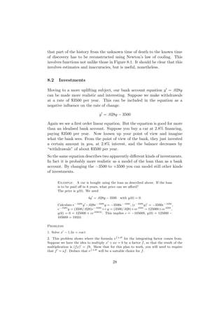
![3. The temperature of an apple pie is recorded as a function of time. It begins in the
oven at 450 degrees, and is moved to an 80 degree kitchen. Later it is moved to a 40
degree refrigerator, and finally back to the 80 degree kitchen. Make a sketch somewhat
like Figure 8.1, which shows qualitatively the temperature history of the pie.
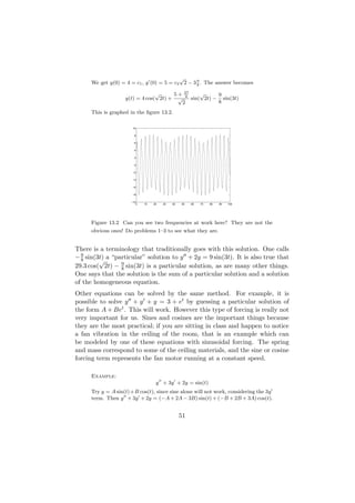
4. A body is found at midnight, on a night when the air temperature is 16 degrees C. Its
temperature is 32 degrees, and after another hour, its temperature has gone down to 30.5
degrees. Estimate the time of death.
5. Sara’s employer contributes $3000 per year to a retirement fund, which earns 3%
interest. Set up and solve an initial value problem to model the balance in her fund, if it
began with $0 when she was hired. How much money will she have after 20 years?
6. Show that the change of variables x = 1/y converts the logistic equation y = .028(y −
y 2 ) of Lecture 4 to the first order equation x = −.028(x − 1), and figure out a philosophy
for why this might hold.
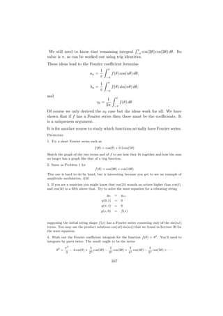
7. A rectangular tank measures 2 meters east-west by 3 meters north-south and contains
water of depth x(t) meters, where t is measured in seconds. One pump pours water in
at the rate of 0.05 [m3 /sec] and a second variable pump draws water out at the rate of
0.07 + 0.02 cos(ωt) [m3 /sec]. The variable pump has period 1 hour. Set up a differential
equation for the water depth, including the correct value of ω.
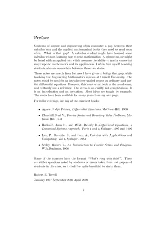
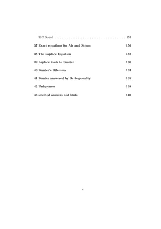
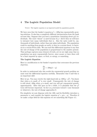
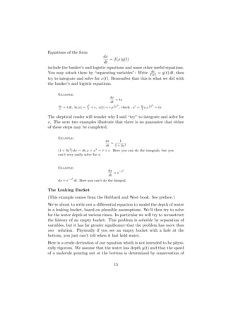
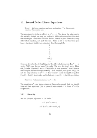
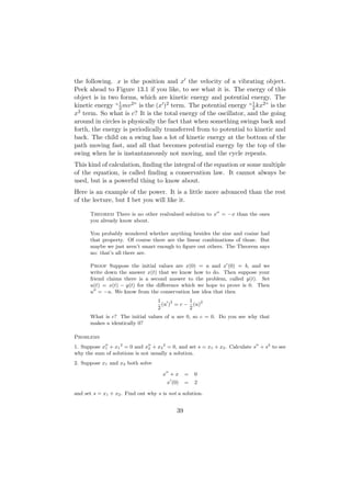
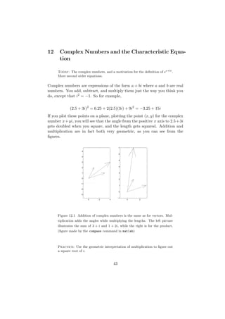
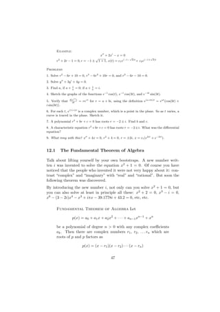
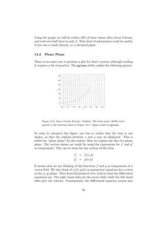
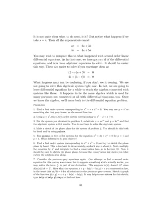
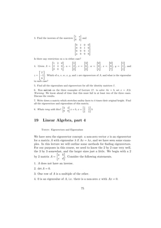
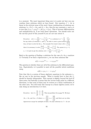
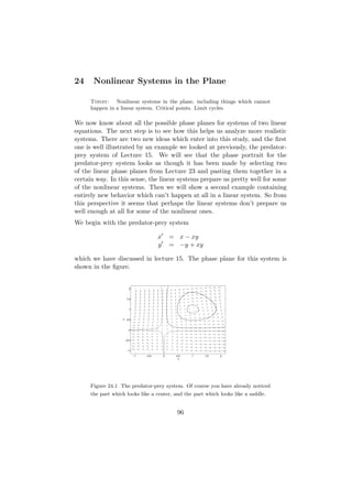
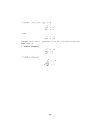
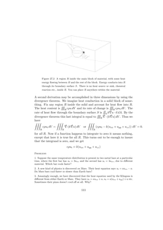
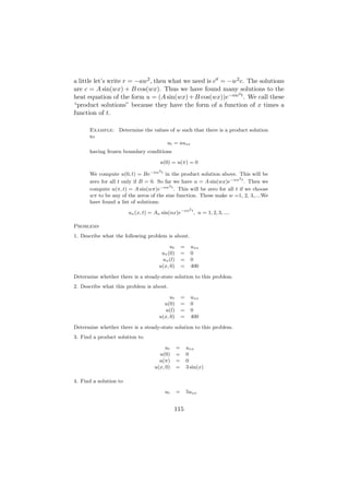
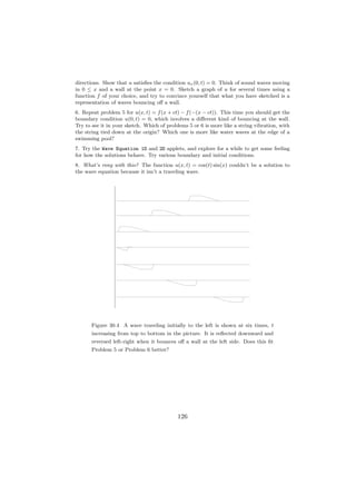
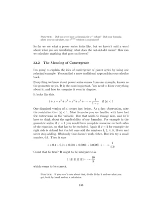
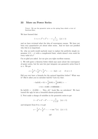
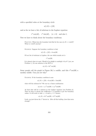
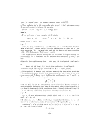
x
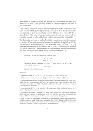
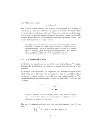
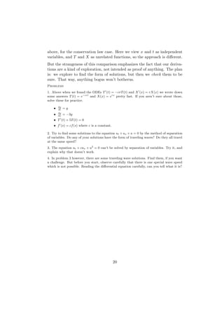
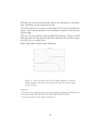
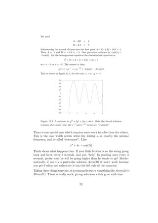
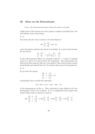
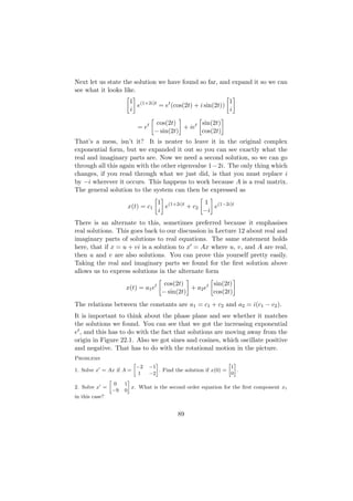
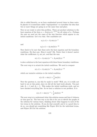
Figure 8.2 Here x(t) is the length of a line of people waiting to buy tickets.
Is the rate of change proportional to the amount present? Does the ticket
seller work twice as fast when the line is twice as long?
29](https://image.slidesharecdn.com/dn-120926135951-phpapp02/85/Dn-35-320.jpg)
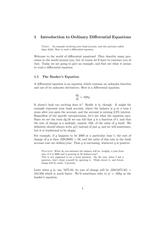
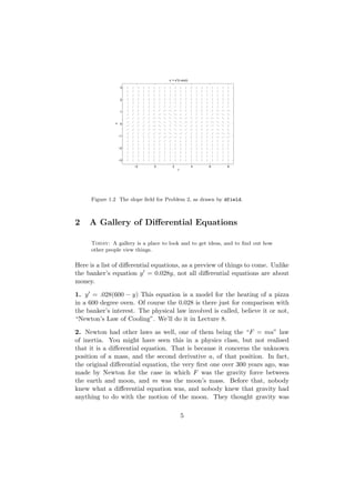
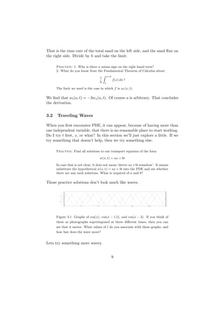
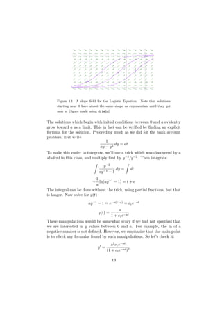
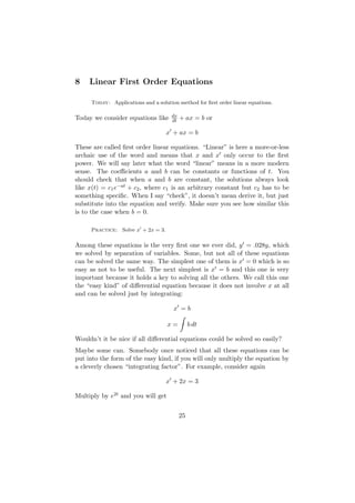
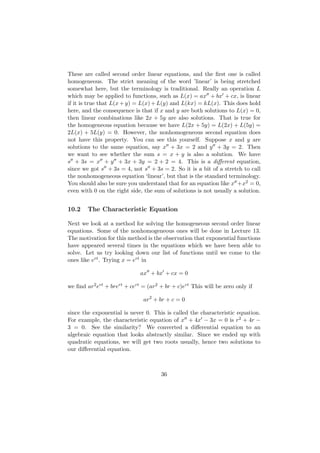
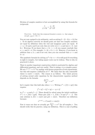
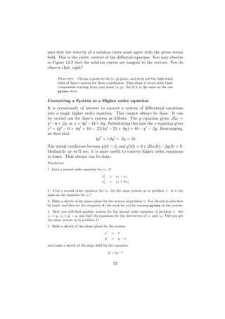
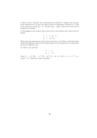
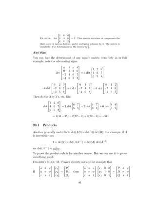
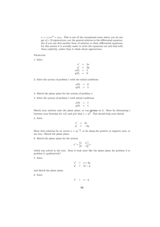
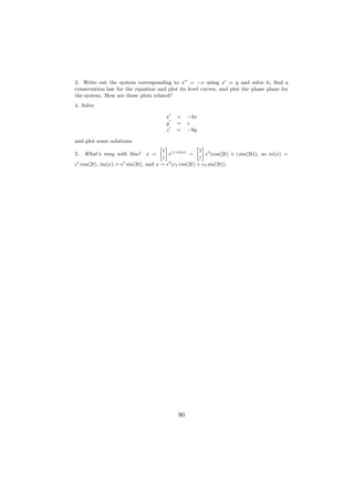
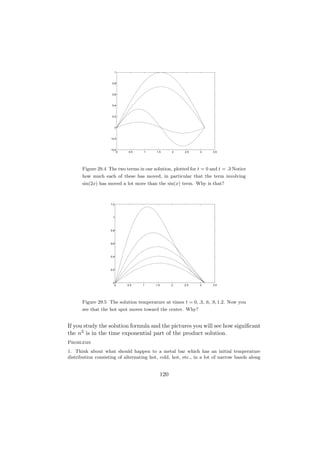
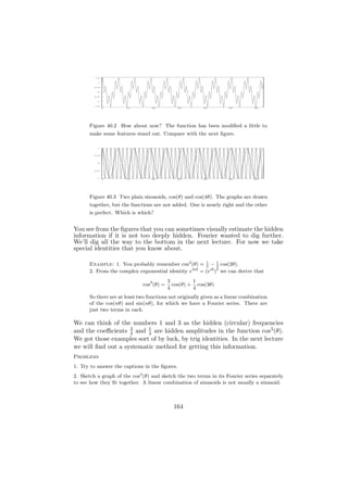
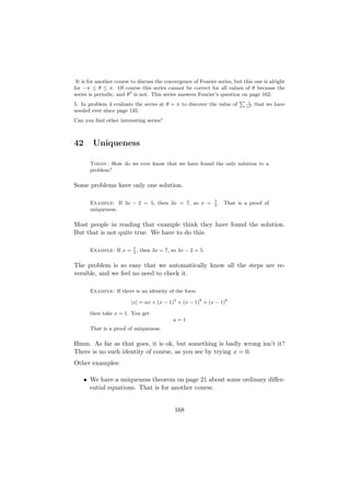
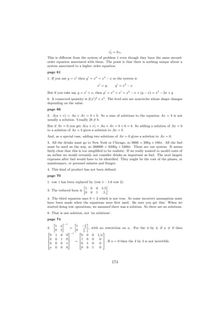
![9 [oiler’s] Euler’s Numerical Method
Today: A numerical method for solving differential equations either by
hand or on the computer, several ways to run it, and how your calculator
works.
Today we return to one of the first questions we asked. “If your bank balance
y(t) is $2000 now, and dy/dt = .028y so that its rate of change is $56 per
year now, about how much will you have in one year?” Hopefully you guess
that $2056 is a reasonable first approximation, and then realize that as soon
as the balance grows even a little, the rate of change goes up too. The
answer is therefore somewhat more than $2056.
The reasoning which lead you to $2056 can be formalised as follows. We
consider
x = f (x, t)
x(t0 ) = x0
Choose a “stepsize” h and look at the points t1 = t0 + h, t2 = t0 + 2h,
etc. We plan to calculate values xn which are intended to approximate the
true values of the solution x(tn ) at those time points. The method relies on
knowing the definition of the derivative
x(t + h) − x(t)
x (t) = lim
h→0 h
We make the approximation
. xn+1 − xn
x (tn ) =
h
Then the differential equation is approximated by the difference equation
xn+1 − xn
= f (xn , tn )
h
Example: With h = 1 the bank account equation becomes
yn+1 − yn
= .028yn
h
or
yn+1 = yn + .028hyn
30](https://image.slidesharecdn.com/dn-120926135951-phpapp02/85/Dn-36-320.jpg)
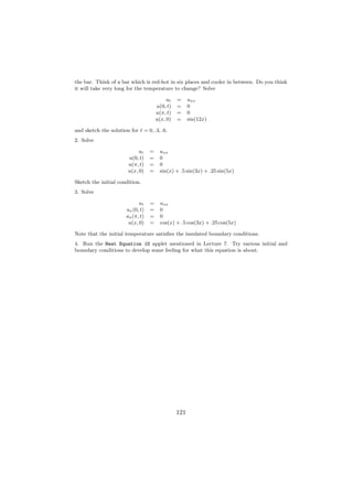
![For additional practice you should vary h and the equation to see what happens.
There are also more sophisticated methods than Euler’s. One of them is
built into matlab under the name ode23 and you are encouraged to use it
even though we aren’t studying the internals of how it works. You should
type help ode23 in matlab to get information on it. To solve the carrier
problem using ode23, you may proceed as follows. Use the same myfunc.m
file as before. Then in Matlab give the commands
[t,p] = ode23(’myfunc’,0,60,.08);
plot(t,p)
Your results should be about the same as before, but generally ode23 will
give more accuracy than Euler’s method. There is also an ode45. We won’t
study error estimates in this course. However we will show one more example
to convince you that these computations come close to things you already
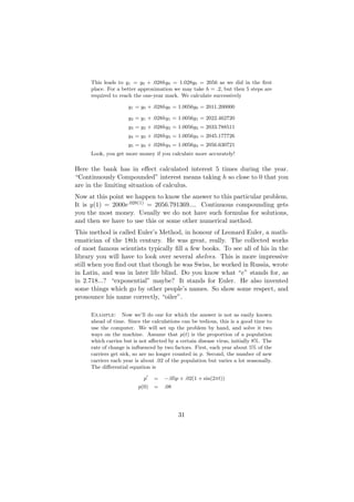
know. Look again at the simple equation x = x, with x(0) = 1. You know
the solution to this by now, right? Euler’s method with step h gives
xn+1 = xn + hxn
This implies that
x1 = (1 + h)x0 = 1 + h
x2 = (1 + h)x1 = (1 + h)2
···
xn = (1 + h)n
Thus to get an approximation for x(1) = e in n steps, we put h = 1/n and
receive
. 1
e = (1 + )n
n
Let’s see if this looks right. With n = 2 we get (3/2)2 = 9/4 = 2.25. With
.
n = 6 and some arithmetic we get (7/6)6 = 2.521626, and so forth. The point
is not the accuracy right now, but just the fact that these calculations can be
done without a scientific calculator. You can even go to the grocery store,
find one of those calculators that only does +–*/, and use it to compute
important things.
Did you ever wonder how your scientific calculator works? Sometimes people
think all the answers are stored in there somewhere. But really it uses ideas
33](https://image.slidesharecdn.com/dn-120926135951-phpapp02/85/Dn-39-320.jpg)
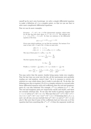

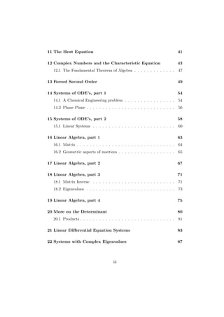
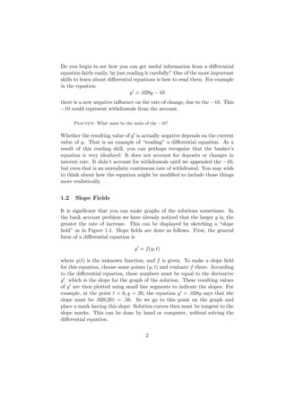
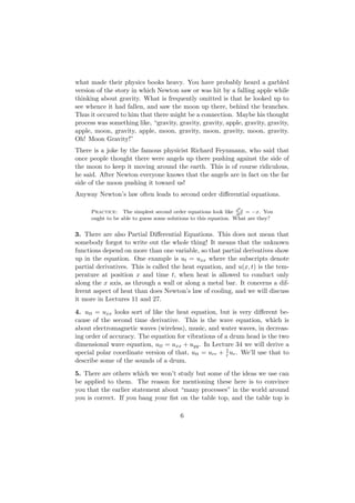
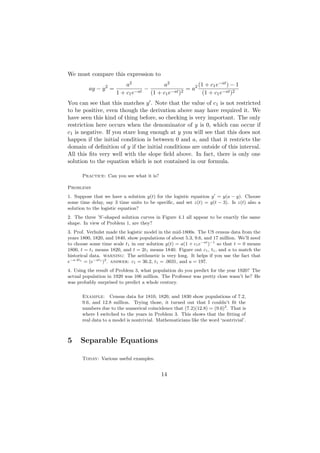
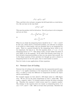
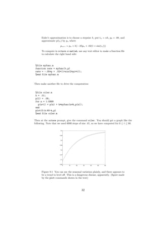
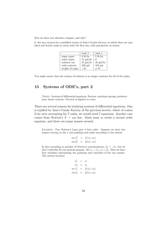
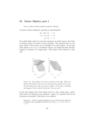
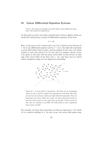
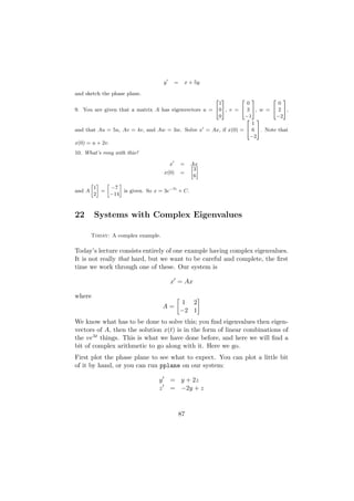
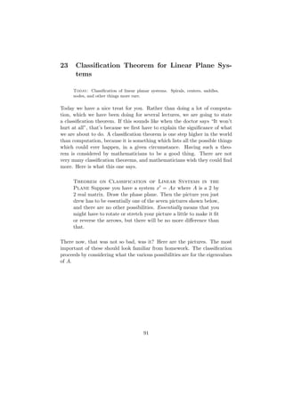
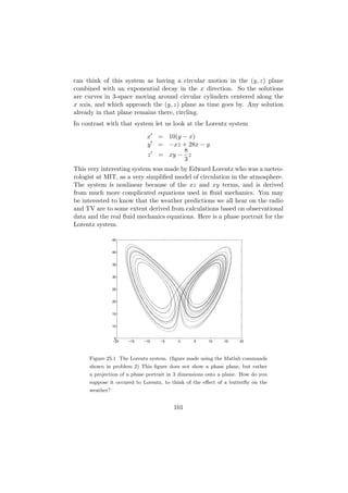
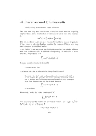
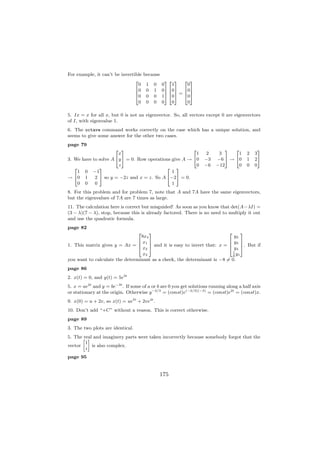
![14 Systems of ODE’s, part 1
Today: Why would anybody want to study more than one equation at a
time? Find out. Phase plane.
14.1 A Chemical Engineering problem
Jane’s Candy Factory contains many things of importance to chemical en-
gineers. One of the processing lines contains two tanks of sugar solution.
Pure water and sugar continually enter the first one where they are mixed,
and an equal volume of the solution flows to the second, where more sugar
is added. The solution is taken out at the same rate from the second tank.
The flow rates are as shown in the table.
tank 1 tank 2
sugar input 10 lb/hr 6 lb/hr
water input 25 gal/hr 0
solution out 25 gal/hr 25 gal/hr
tank contents 100 gal 125 gal
weight of sugar x lb y lb
Jane’s control system tracks the weight of sugar present in the tanks in the
variables x and y. We can figure out the rates of change easily. The basic
principle here is conservation of mass.
x [lb]
x [lb/hr] = the rate in − the rate out = 10 [lb/hr] − (25 [gal/hr])
100 [gal]
See, you just keep an eye on the units, and everything works out. Similarly
x y
y =6+ (25) − (25)
100 125
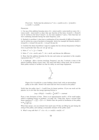
Jane would like to predict the length of time required to start up this system,
i.e., beginning with pure water in brand new tanks, how long before a “steady
state” condition is reached (if ever)? This is an initial value problem:
x = 10 − .25x
y = 6 + .25x − .2y
x(0) = 0, y(0) = 0
54](https://image.slidesharecdn.com/dn-120926135951-phpapp02/85/Dn-60-320.jpg)
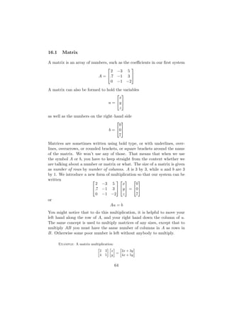
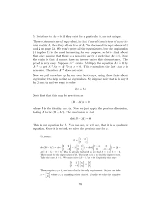
![2 32 3 2 3
2 −3 5 1 12
4.7 −1 3 5 405 = 46.75
0 −1 −2 2 −4
» –» – » –
1 2 a b 1a + 2c 1b + 2d
=
3 4 c d 3a + 4c 3b + 4d
1 0 0
1 0
I is the special matrix or 0 1 0 or . . . , one for each size. It is
0 1
0 0 1
the identity matrix and you should check that always AI = IA = A, Iu = u.
It is also useful to abbreviate the system Au = b further by not writing the
variables at all: the 3 by 4 matrix [A b] is called the augmented matrix of
the system. In general, if you have a system of m equations in n unknowns,
Au = b, then A is m by n, b is n by 1, u is m by 1, and the augmented
matrix [A b] is m by (n + 1).
16.2 Geometric aspects of matrices
Before continuing with equation–solving, there are several remarks. Matrices
like
x
u = y
z
which consist of one column are sometimes called column vectors, and pic-
tured as an arrow from the origin to the point with coordinates (x, y, z).
In other words, u here has exactly the same meaning as xı + y + z k, and
you can think of it in exactly the same way. Of course we are now allowing
our column vectors to contain more than three coordinates, so the three–
dimensional vector notation doesn’t carry over. Welcome to the fourth di-
mension! There are some very nice geometric ideas connected to this form of
multiplication. These seem at first very different and unrelated to equation–
solving. We’ll give one example now, just so you realise that there are several
different reasons for studying matrices. Consider the simple matrix
1 0
A= 1
0 2
A can be applied to any “point” (x, y) in the plane by using multiplication:
x x
A = y
y 2
65](https://image.slidesharecdn.com/dn-120926135951-phpapp02/85/Dn-71-320.jpg)
![17 Linear Algebra, part 2
Today: Row Operations
Now that our matrix notation is established, we turn to the question of
solving the linear system Au = b. You may have solved such things in
algebra courses in the past, by eliminating one variable at a time. This
works fine for systems of 2 or maybe 3 equations. For our purposes though,
it is important to learn a very systematic way of accomplishing this. We
will describe a procedure which applies equally well to systems with any
number of variables. In case you are wondering about the need for that,
let me reassure you that linear algebra, of all the things you study, might
be one thing that gets used in real life. Consider an airline company which
needs to keep track of 45000 passengers, 200 planes, 300 crews, 8500 spare
parts, 25 cities, 950000 pounds of jet fuel, 85600 soft drinks, etc, etc. Then
there are the airframe engineers who compute the airflow at 10000 points
around the plane, and the engine people who compute the temperature and
gas flow at 3000 points inside the engines, and you get the picture.
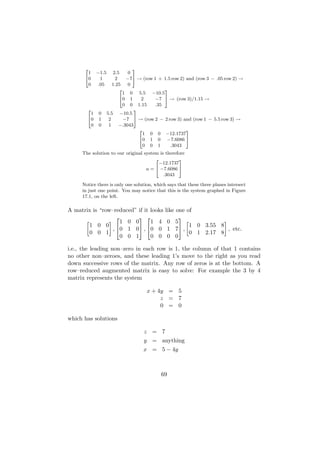
Before we describe row operations, you should see what the system of equa-
tions looks like in a special case like
1 0 0 5
0 1 0 7
0 0 1 9
This is the augmented matrix for the system x = 5, y = 7, and z = 9.
There is nothing to solve in this case. Consequently, the object of these row
operations is to put the matrix into the form [I b] if possible.
We now describe “row operations” for solving the system Au = b. There
are three row operations, which are applied to the augmented matrix [Ab],
and have the effect of manipulating the various equations represented by the
augmented matrix.
1) A row may be multiplied by a non–zero number.
2) Two rows may be interchanged.
3) A row may be replaced by its sum with a multiple of another row.
Row operations do not change the solutions of the system. This is clear for
the first two, and requires a bit of thought for the third one. They only
change the appearance of the equations.
67](https://image.slidesharecdn.com/dn-120926135951-phpapp02/85/Dn-73-320.jpg)
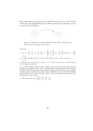
![A system may have many solutions.
Example: The system » –» – » –
2 3 x 1
=
4 6 y 2
represents the two lines 2x + 3y = 1 and 4x + 6y = 2. You might notice that
these are two equations for the same line. Therefore any point on this line
should be a solution to both equations. Let’s do the row operations and see
what happens. We have the augmented matrix
» – » –
2 3 1 2 3 1
→ (row 2 − 2 row 1) →
4 6 2 0 0 0
Here we have replaced row 2 by (row 2)–2(row 1). Look at the bottom line.
It says that 0x + 0y = 0. That is true but not helpful. The top line says
that 2x + 3y = 1. Since this is the only requirement for a solution, there are
indeed infinitely many solutions
1 3
x = − y
2 2
y = anything
A system may have no solutions.
Example: The system » –» – » –
2 3 x 0
=
4 6 y 2
has augmented matrix
» – » –
2 3 0 2 3 0
→ (row 2 − 2 row 1) →
4 6 2 0 0 2
Look at the bottom line. It says that 0x + 0y = 2. Is that possible? (No.)
So this system has no solution. It describes two parallel lines.
The next example involves a bit more arithmetic, and is our original system.
It shows that a system may have a unique solution.
Example:
2 3 2 3
2 −3 5 0 1 −1.5 2.5 0
[A b] = 4.7 −1 3 05 → (.5 row 1) → 4.7 −1 3 05 → (row 2 − .7 row 1) →
0 −1 −2 7 0 −1 −2 7
2 3
1 −1.5 2.5 0
40 .05 1.25 05 → (interchange row 2 and row 3) and (−row 2) →
0 −1 −2 7
68](https://image.slidesharecdn.com/dn-120926135951-phpapp02/85/Dn-74-320.jpg)
![7. Same instructions as problem 5 for the system
x − y + z − 2w = 0
x+y+z−w = 1
−x − y = 2
8. Whats rong with this?
x + 2y = 0
3y = 0
gives y = 0, then x = 0. Therefore there are no solutions.
18 Linear Algebra, part 3
Today: Matrix inverse, solutions to linear sytems in matlab, and the Eigen-
value concept
18.1 Matrix Inverse
We learned last time about solving a system Ax = b by row operations – you
row reduce the augmented matrix [A b] and read the solutions, if there are
any. There is another approach which is harder to compute but helpful to
know about sometimes. It goes like this. We try to solve Ax = b by analogy
with the arithmetic problem 2x = 7. In arithmetic the answer is x =
2−1 7. Here there is sometimes a matrix which deserves to be named A−1 , so
that the solution might be expressed as x = A−1 b. A−1 is pronounced “A
inverse”. Wouldn’t that be nice? Yes, it would be nice, but we’ll see some
reasons why it can’t work in every case. It can’t work in every case because,
among other things, it would mean that there is a unique answer x, and we
have already seen that this is not at all true! Recheck the examples in the
previous sections if you need a reminder of this point. Some systems have
no solutions, some have one, and some have infinitely many. It turns out
that for some matrices A, the inverse A−1 does exist. All of these matrices
are square, and satisfy some additional restrictions which we will list below.
Before getting to that list though, return to the phrase used above, “a matrix
which deserves to be named A−1 ”. What does that mean? We’ll say that
a matrix B is an inverse of matrix A if AB = BA = I. This is the key
property. In fact, there can only be one matrix with this property: if B and
C both have this property, then B = BI = BAC = IC = C. Since there is
only one, we can name it A−1 .
71](https://image.slidesharecdn.com/dn-120926135951-phpapp02/85/Dn-77-320.jpg)
![» – » – » –
1 0 1 0 1 0
Example: For A = 1 and B = , we have AB = =I
0 2
0 2 0 1
and BA = I. So » –−1 » –
1 0 1 0
1 =
0 2
0 2
and » –−1 » –
1 0 1 0
= 1
0 2 0 2
» – » – » –
2 5 3 −5 1 0
Example: For A = and B = , we have AB = =
1 3 −1 2 0 1
I and BA = I. So » –−1 » –
2 5 3 −5
=
1 3 −1 3
and » –−1 » –
2 −5 2 5
=
−1 3 1 3
It turns out that there is a formula for the inverse of a 2 by 2 matrix, but
that there is no really good formula for the larger ones. It is:
−1
a b 1 d −b
= IF ad − bc = 0.
c d ad − bc −c a
a b x y
You can derive this formula yourself: try to solve = I for
c d z w
x, y, z, and w in terms of a, b, c, and d, and you will get it eventually.
The number ad − bc is called the “determinant” of the matrix, because it
determines whether or not the matrix has an inverse.
Practice: You should check that this formula for the inverse agrees with
the earlier examples.
We also are going to record the method used to find inverses of larger matri-
ces. They may be found, when they exist, by row operations. You write the
large augmented matrix [A I] which is n by 2n if A is n by n. Then do row
operations, attempting to put it into the form [I B]. If this is possible, then
B = A−1 . If this is not possible, then A−1 does not exist. The rationale for
this method is left for a later course in linear algebra, but you can consider
for yourself what equations are really being solved, when you use this large
augmented matrix.
72](https://image.slidesharecdn.com/dn-120926135951-phpapp02/85/Dn-78-320.jpg)
![2 3
−1 0 0
Example: For A = 4 2 1 05 we do operations:
0 0 4
2 3
−1 0 0 1 0 0
[A I] = 4 2 1 0 0 1 05 → −(row 1) and (1/4)(row 3) and (row 2 + 2 row 1) →
0 0 4 0 0 1
2 3
1 0 0 −1 0 0
40 1 0 2 1 0 5
0 0 1 0 0 .25
2 32 3
−1 0 0 −1 0 0
You can check that 4 2 1 05 4 2 1 0 5=I
0 0 4 0 0 .25
Have you heard about people who “only know enough to be dangerous”? It
means they have some special knowledge of something, but without enough
depth to use it properly. octave and matlab provide a tool to put you into
this category. Isn’t that exciting? So we hope that you will not get hurt
if you know the following: the program can sometimes solve Au = b if you
simply type u = Ab. That is a backward division symbol, intended to
suggest that one is more–or–less dividing by A on the left. It mimics the
notation u = A−1 b. In the problems, we suggest trying this to see what it
produces in several cases.
18.2 Eigenvalues
Usually when you multiply a vector by a matrix, the product has a new
length and direction, as we saw with the little smiley faces: If u is a vector
from the origin to the left eye on page 66 then Au points in a different
direction from u. This is typical. On the other hand, let v be the vector
from the origin to the top of Smiley’s head. In this case, we see that Av = 1 v.
2
This is not typical, it is special, and turns out to be quite important. Try
to locate other vectors with this special property, that
Av = λv
A vector v = 0 which has this property, for some number λ (“lambda”), is
called an eigenvector of A, and λ is called an eigenvalue. Eigen is a German
word which means here that these things are characteristic property of the
matrix. You may notice that we excluded the zero vector. That is because
it would work for every matrix, and therefore not be of any interest. It is ok
73](https://image.slidesharecdn.com/dn-120926135951-phpapp02/85/Dn-79-320.jpg)
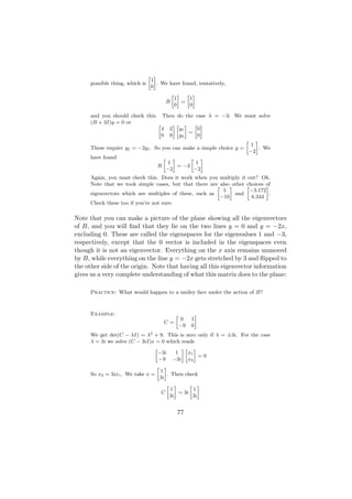
![For the case λ = −3i, the only change is to replace i by −i everywhere, and
check that » – » –
1 1
C = −3i
−3i −3i
Note that for C, one has run into complex numbers, and so the nice ge-
ometric interpretation which was available in the plane for B is no longer
available. Two complex numbers are about the same as four real numbers,
so you might have to imagine something in four dimensions in order to
visualize the action of C in the same sense as we were able to visualize B.
Practice: It does make sense, nevertheless, that not all 2 by 2 matrices
can be thought of as stretching vectors in the plane: figure out what what
C does to smiley faces, if you want to understand this point better.
Larger Matrices
The procedure for 3 by 3 and larger matrices is similar to what we just did
for 2 by 2’s. The main thing which needs to be filled in is the definition of
determinant for these larger matrices. We do not want to get involved with
big determinants in this class. To find eigenvalues for a 3 by 3 matrix you
can look up determinants in your calculus book, or remember them from
high school algebra. Also see Lecture 20. There is also a possibility of using
some routines which are built into octave. These work as follows. Suppose
we have a matrix
1 2 3
A = 4 5 6
7 8 9
To approximate the eigenvalues of A you can type the following commands:
A=[1 2 3;4 5 6;7 8 9];
eig(A)
To get eigenvector approximations also you may type
[V D]=eig(A)
This creates a matrix V whose columns are approximate eigenvectors of A,
and a matrix D which is a “diagonal” matrix having approximate eigenvalues
along the main diagonal. For example, D in this case works out to be
16.1168 0 0
D= 0 −1.1168 0
0 0 0
78](https://image.slidesharecdn.com/dn-120926135951-phpapp02/85/Dn-84-320.jpg)
![and taking determinants you get a formula for the answer:
P b c
det(A)x1 = det D v w
Q s t
Similary for x2 and x3 , and for any size system. Cramer’s rule is an inter-
esting theoretical tool these days, but not computationally efficient because
it takes too long to work out determinants.
Problems
1. Is this matrix invertible? 2 3
0 0 0 8
61 0 0 07
6 7
40 1 0 05
0 0 1 0
2. If a 2 by 2 matrix A has columns v and w we will write A = [v w] and think of the
determinant as a function of the two columns f (v, w) = det(A). Convince yourself that
f (au + bv, w) = af (u, w) + bf (v, w)
whenever u, v, and w are vectors and a and b are numbers.
We say that det is a linear function of the first column of the matrix.
3. Of course det is a linear function of the second column too. Figure out why that makes
this kind of identity hold:
f (au + bv, cw + dz) = acf (u, w) + adf (u, z) + bcf (v, w) + bdf (v, z)
82](https://image.slidesharecdn.com/dn-120926135951-phpapp02/85/Dn-88-320.jpg)
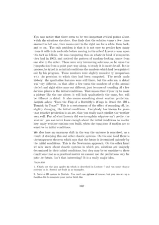
![% file ef.m
function vec=ef(t,w)
vec(1)=10*(w(2)-w(1));
vec(2)=-w(1)*w(3)+28*w(1)-w(2);
vec(3)=w(1)*w(2)-8*w(3)/3;
% end file ef.m
Then give commands like
[t, w] = ode45(’ef’,0,20,[5 7 9]);
plot(w(:,1),w(:,3))
This will compute the solution to the Lorentz system for 0 ≤ t 3 20 with initial conditions
2 ≤
x
(5, 7, 9), and make a plot. The symbol w was used here for 4y 5, so what was plotted was
z
x versus z. Naturally you can play with the plot command to get different views. The
hardest part is understanding why w(:, 1) means x. You have to realize that w is a list of
three lists, before it makes any sense. Change these files to solve a system of your choice.
Note that you are not restricted to just three dimensions either.
3. Change the plot command in problem 2 to plot x versus t.
4. Change the ef.m file of problem 2 to solve the linear system described in the text. You
will have to play with the plot command to get a nice perspective view, for example you
can plot x versus y + 2z or something like that. Does the picture fit the description given
in the text?
5. What’s rong with this? According to this lecture, if you have a system of 3 or more
variables you can get chaos. And, according to Lecture 15, if you have a system of 2
spring-masses, you get 2 Newton’s laws or a system of 4 first-order equations. Therefore
2 spring-masses are always chaotic.
103](https://image.slidesharecdn.com/dn-120926135951-phpapp02/85/Dn-109-320.jpg)
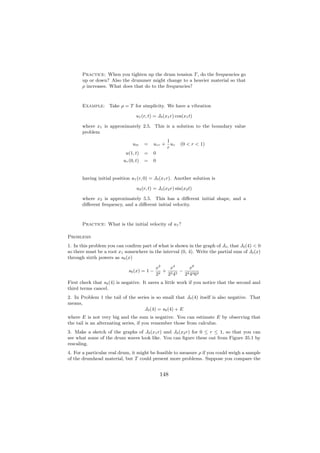
![26 Boundary Value Problems
Today: A change from initial conditions. Boundary values. We find that
we don’t know everything about y = −y after all.
You have by now learned a lot about differential equations, or to be more
specific, about initial value problems for ordinary differential equations. You
have also seen some partial differential equations. In most cases we have
had initial conditions. At this time we are prepared to make a change, and
consider a new kind of conditions called boundary conditions. These are
interesting both for ODE, and also in connection with some problems in
PDE.
First you have to know what a boundary is. It is nearly the same thing in
mathematics as on a map: the boundary of a cube consists of its six faces,
the boundary of Puerto Rico is its shore line, the boundary of the interval
[a, b] consists of the two points a and b. The concept of a boundary value
problem is to require that some conditions hold at the boundary while a
differential equation holds inside the set. Here is an example.
Example:
y = −y
y(0) = 0
y(2π) = 0
We are asked to solve a very familiar differential equation, but under very
unfamiliar conditions. The function y is supposed to be 0 at 0 and π. The
differential equation here has solutions y = A cos(t) + B sin(t). We apply the
first boundary condition, giving y(0) = 0 = A. So we must take A = 0. That
was easy! Now apply the second boundary condition, giving y(2π) = 0 =
B sin(2π). Well, it just so happens that the sin(2π) is zero. So the second
boundary condition is fulfilled no matter what B is. Answer: y(t) = B sin(t),
B arbitrary.
Notice how different this example was from our experience with initial con-
ditions, that there were infinitely many solutions. Just the opposite thing
can happen too:
Example:
y = −y
y(0) = 0
y(6) = 0
104](https://image.slidesharecdn.com/dn-120926135951-phpapp02/85/Dn-110-320.jpg)
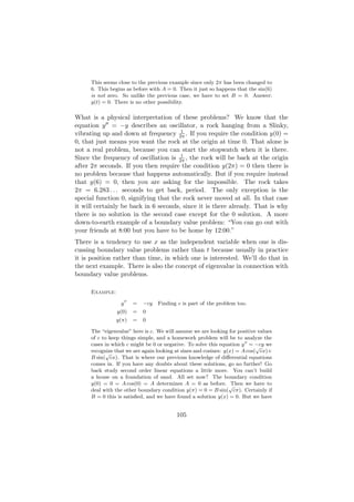
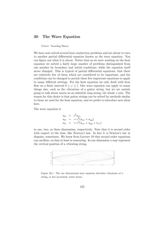
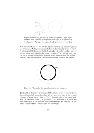
![31 Beams and Columns
Today: A description of some differential equations for beams and columns.
Figure 31.1 A beam with some exaggerated deflection.
A beam is a bar loaded transverse to the axis, while a column is loaded along
the axis. Of course the orientation doesn’t matter even though we think of
a column as being vertical,
F
P
V y
1
M
R
Figure 31.2 Left: A segment of the beam, with shearing force V and moment
M acting. R is the radius of curvature.
Right: A column buckled by an applied force.
For either case suppose x axis left to right gives position along the bar, and
we have a segment of the bar as shown with shear force V [Newtons] and
bending moment M [Newton-meters] as functions of x. Also F [N/m] is
127](https://image.slidesharecdn.com/dn-120926135951-phpapp02/85/Dn-133-320.jpg)
![For example a q × q square cross section beam has moment of inertia I =
q/2 q/2 2 4
−q/2 −q/2 y1 dy1 dy2 = q /12.
The easier parts are to see that M is proportional to the shear V , and that
V is proportional to F , the downward load [N/m] applied to the beam.
Practice: For M sum moments about the left end point of the segment,
giving −M (x) + M (x + ∆x) + (∆x)V (x + ∆x) = 0. For V sum downward
forces on the segment, giving −V (x) + V (x + ∆x) + F (x)(∆x) = 0. Then
divide by ∆x and take limits as ∆x → 0.
Putting all that together we summarize beams: (sign conventions may differ
in various texts)
EIy = M, EIy = −V, EIy =F
These are differential equations, and in addition they tell us how to interpret
various boundary conditions. For example a cantilever beam embedded
solidly into concrete at one end probably has y = y = 0 at the concrete
end, and y = y = 0 at the free end.
Two more applications:
For a column which is deflected into a bent shape y(x) by an axial force P ,
you get a bending moment y(x)P at each cross section, and taking account
of signs the DE becomes
EIy = −P y
Finally we mention vibrating beams: Suppose y depends on x and t and
that there is no applied load F . If the mass of the beam is ρ [kg/m] then
you find a PDE
EIyxxxx = −ρytt
for the vibrations.
Problems
1. Find a type of boundary value problem in Lecture 26 which could be applied to the
P
column. Take EI = 1 if that helps. What is the smallest eigenvalue at which the column
buckles?
2. Try to find some beam vibrations of the form
y(x, t) = a cos(bt) sin(cx)
That does not mean ‘derive this formula from scratch’. It means plug it into the beam
equation
ρytt = −EIyxxxx
129](https://image.slidesharecdn.com/dn-120926135951-phpapp02/85/Dn-135-320.jpg)
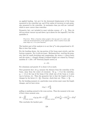
![1. What is the radius of convergence of
1 + x + x2 + x3 + · · ·?
(Whatever you do, don’t apply the ratio test to this series. The ratio test is proved based
on what we already know about this series.)
Does it converge when x = − 1 ? To what?
3
2. What does the power series theorem give for the radius of convergence of the derivative
series
1 + 2x + 3x2 + 4x3 + · · · = (1 + x + x2 + x3 + x4 + · · · ) ?
Does it converge when x = − 1 ? To what?
3
3. What is the radius of convergence of
1 + (x − 10) + (x − 10)2 + (x − 10)3 + · · ·?
Does it converge when x = 8.3?
4. Use your knowledge of the cosine function to figure out the value of
π2 π4 π6
1− + − + ···
2 4! 6!
It really wouldn’t pay to evaluate the first few terms of that, would it?
34 Power Series used: A Drum Model
Today: We set up a model for the vibrations of a drum head.
The Drum
Our model of a drumhead has radius 1, and it only vibrates in circular
symmetry. That means you can only hit it in the center, so to speak. Using
polar coordinates, there is dependence on r and t but not on θ. We write
u(r, t)
for the upward displacement of the drumhead out of its horizontal resting
plane, and assume that u is small and that
u(1, t) = 0
since the edges of the head are pulled down against the rim of the drum.
We will assume that there is a tension T [N/m] uniformly throughout the
drumhead. Convince yourself that this is reasonable as follows. Imagine
the tension forces on a small triangle of material located anywhere in the
drumhead.
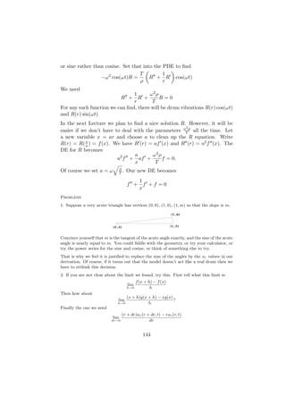
141](https://image.slidesharecdn.com/dn-120926135951-phpapp02/85/Dn-147-320.jpg)
![T
T
r r+dr
Figure 34.2 A cut through the annular region, viewed on edge. The ver-
tical displacement is greatly exaggerated. We’re accounting for the vertical
components of the tension forces.
The net force vertically is then
T (2π)(r + dr)ur (r + dr, t) − T (2πr)ur (r, t)
The acceleration of the annulus is utt . Mr. Newton says that we also need
its mass. The mass of the segment is its area times its density ρ [kg/m2 ], or
ρ π(r + dr)2 − πr2 By Newton then
T (2π)(r + dr)ur (r + dr, t) − T (2πr)ur (r, t) = ρπ(2r dr + (dr)2 )utt
∂(T rur )
Divide by dr and take dr → 0 getting ∂r = ρrutt .
T
So our equation is rutt = ρ (rur )r or equivalently
T 1
utt = urr + ur
ρ r
We will find some solutions to this having u(1, t) = 0 at the rim of the
drum. The solutions will be vibrations of our drum model, and hopefully
will resemble vibrations of a real drum.
Practice: Polar coordinates are awkward at the origin. What should the
slope ur (0, t) be at the center, so that the shape of the drumhead is smooth
there?
Separation of Variables
Maybe our wave equation has some product solutions of the form u(r, t) =
R(r)T (t). Since this is supposed to represent music, lets try
u(r, t) = R(r) cos(ωt)
143](https://image.slidesharecdn.com/dn-120926135951-phpapp02/85/Dn-149-320.jpg)
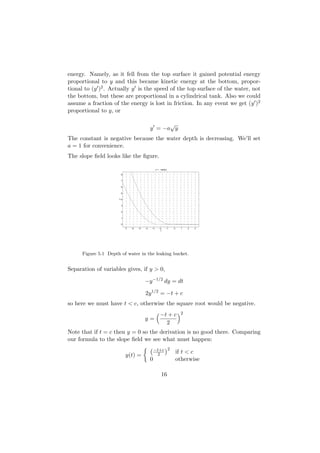
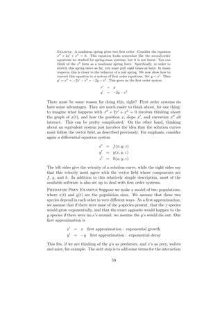
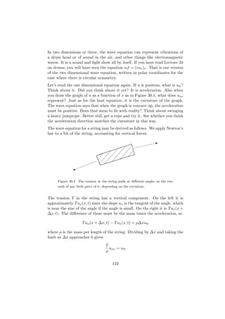
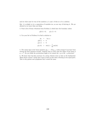
![1
0.8
0.6
0.4
0.2
0
-0.2
-0.4
0 5 10 15 20 25 30 35 40
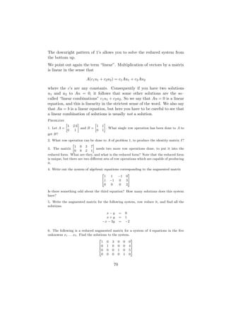
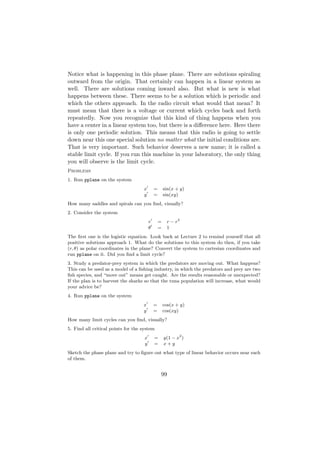
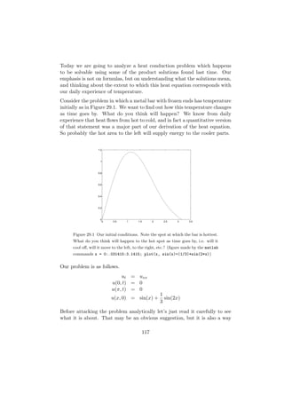
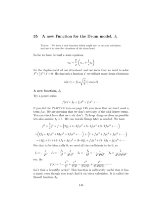
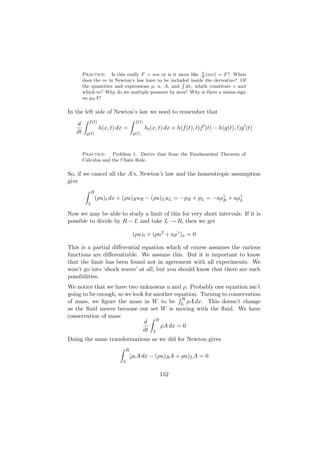
x2 x4 x6
Figure 35.1 Graph of Bessell J0 (x) = 1 − 22
+ 22 42
− 22 42 62
+ ···
So f (x) = J0 (x) or, if we need a multiple of that, f (x) = f0 J0 (x) for some
constant f0 . We need to know what this function is like, to see whether it
gives us plausible drumhead vibrations
ρ
u(r, t) = f0 J0 (ω r) cos(ωt)
T
The series tells us some of the properties that we need, and the differential
equation
1
J0 + J0 + J0 = 0
x
itself gives other properties.
First the series: The series is reminiscent of that for the cosine function, so
maybe J0 has many zeros, and oscillates, and is periodic. Well, 2 out of
3 isn’t bad: J0 has infinitely many zeros and oscillates somewhat like the
cosine function, but is not periodic. In a homework problem you will use the
series to find that J0 (4) is negative. Since we know J0 (0) = 1, there must
be a number x1 between 0 and 4 where J0 (x1 ) = 0. In fact the first root x1
is roughly 2.5 and the second root x2 is near 5.5, x3 is about 8.5, and there
are infinitely many others.
From the DE we see this: suppose you have an interval like [x1 , x2 ] where
J0 is 0 at each end, and nonzero between. At any local min or max where
J0 = 0, The DE then tells that J0 = −J0 there. The graph can’t be concave
up at a local max, nor concave down at a minimum. So the graph can only
have simple humps like the cosine does, no complicated zig-zags between the
roots.
146](https://image.slidesharecdn.com/dn-120926135951-phpapp02/85/Dn-152-320.jpg)
![sound of the drum to a piano or guitar and decide that the fundamental tone is near the
note A2 = 110 [cycles/sec], the next to lowest string on a guitar. Figure out T for this
ρ
drum.
5. Remind yourself that the first three tones of a string have frequencies in the proportion
1 : 2 : 3, i.e., there are solutions cos(t) sin(x), cos(2t) sin(2x), and cos(3t) sin(3x) to the
wave equation ytt = yxx . But what about a drum? Check the graph of J0 and find out
approximately how the lowest three frequencies of a drum are related. This is why pianos
and drums don’t sound the same.
149](https://image.slidesharecdn.com/dn-120926135951-phpapp02/85/Dn-155-320.jpg)
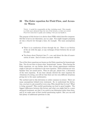
![36.1 The Euler equations
The pipe is full of air. The air velocity is u(x, t) [m/sec], and density ρ(x, t)
[kg/m3 ]. For air, the density is typically around 1.2 near the surface of the
earth, but the velocity could vary over a large range. We can think of x and
u positive toward the right.
111111111111111111
000000000000000000
111111111111111111111111111111111111
000000000000000000000000000000000000
111111111111111111
000000000000000000
111111111111111111111111111111111111
000000000000000000000000000000000000
111111111111111111
000000000000000000
W
111111111111111111
000000000000000000
111111111111111111111111111111111111
000000000000000000000000000000000000
111111111111111111111111111111111111
000000000000000000000000000000000000
L R
Figure 36.1 A portion of air moving in the pipe. The pipe has cross-sectional
area A. The ends L and R don’t have to move at the same speed because
this is compressible flow.
We focus on a portion W of the air. The letters L and R in the figure refer
to the left and right ends of the mass W . W is mathematically just a moving
interval. The left coordinate L is moving at velocity uL , and to be more
precise,
L (t) = u(L(t), t) and uL is an abbreviation for this
and similarly for the right end R at velocity uR .
Besides velocity u(x, t) and density ρ(x, t), we must keep track of the air
pressure p(x, t) [N/m2 ]. It is very easy to mistake ρ and p typographically,
but this won’t happen to you because you are reading very slowly and think-
ing hard, right? The pressure provides forces pL A and pR A on the sides of
W . The homentropic assumption is that the pressure is related to the den-
sity by p = aργ , where γ = 1.4 and a is constant throughout the flow. Aside
from this thermodynamic assumption, the rest of our derivation will consist
of ordinary mechanics.
Newton: The rate of change of momentum of the matter in W is equal to
the sum of applied forces.
R
d
ρuA dx = −pR A + pL A
dt L
151](https://image.slidesharecdn.com/dn-120926135951-phpapp02/85/Dn-157-320.jpg)
![γ−1
Combining the two PDEs in Problem 4, we have wtt = −ρ1 vxt = aγρ1 wxx
or
wtt = c2 wxx
where c2 = aγργ−1 So the pressure disturbance satisfies the wave equation.
1
Practice: What did we just now assume about the second derivatives?
This subtlety is omitted routinely in scientific discussions. Are solutions
to an approximate equation necessarily approximate solutions to the right
equation? This point is also usually omitted.
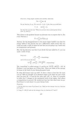
Air pressure at sea level on the earth is about 105 [N/m2 ]. Using this
and previous information, estimate the value of the coefficient c2 occur-
ing in our wave equation. Then, recognizing that traveling waves such as
f (x − bt) + g(x + bt) satisfy a wave equation, what do we learn about the
speed of sound? If lightning strikes at a distance of 3 football fields from
you, how long before you hear it?
Finally, we have to ask: Have we proved anything about the behavior of
real air? What is the criterion for correctness in Physics? in Mathematics?
Have these notes strictly conformed to either?
Loose ends
a) We decided to look for 2 equations for our 2 variables u and ρ. How reliable is the idea
that one needs n equations in n unknowns before you can solve anything? Have you seen
examples in linear algebra, Ax = b, where two equations in three variables might have no
solution? where five equations in three variables might have a unique solution? Think
of the eigenvalue problem Ax = λx, which is nonlinear because we view both λ and x as
unknowns. Suppose A is 8 × 8, how many variables are there? equations? solutions λ?
solutions x? There is some truth in this idea, but few guarantees.
b) You might be wondering whether we need to have another equation about conservation
of energy. Ordinarily we would, but our homentropic assumption p = aργ with no heating
and no friction, has the consequence that all energy changes are accounted for already
by Newton’s law. For a simpler example, a frictionless mass on a spring has Newton’s
law mx = −kx. After multiplying by x you can integrate once to get the conservation
of energy 2 m(x )2 + 1 kx2 = constant. A similar thing happens here. If we were to
1
2
allow heating of the air, then we would need another variable which could be taken to be
temperature, and another equation.
There is plenty of room for misunderstanding about ‘heating’: the word heating means
transfer of heat energy, as through the walls of the pipe. The temperature, which is not
the same as the heating, does in fact change even without heating, because air obeys the
ideal gas law p = 287ρT [mks].
d) We showed that the density disturbance w satisfies the wave equation. You can show
similarly that the velocity disturbance v satisfies the wave equation with the same coeffi-
cient c2 . What is the significance of the fact that the velocity and pressure disturbances
154](https://image.slidesharecdn.com/dn-120926135951-phpapp02/85/Dn-160-320.jpg)
![satisfy the same wave equation? Specifically, is it physically plausible that these two
disturbances might travel at different speeds?
Projects
Project 1. There are at least two R
ways to understand our earlier statement about the mass
L
integral, that the mass in W is R ρA dx. You probably know that you can think of dx
as a bit of length, A dx as a bit of volume, ρA dx as a bit of mass, and the integral adds
them. Another interesting approach is explained by P. Lax in his calculus book. Suppose
we write S(f, I) for the mass contained in interval I = [a, b] when function f gives the
density in I. S has two physically reasonable properties:
1. If I is broken into nonoverlapping subintervals I = I1 ∪ I2 = [a, c] ∪ [c, b], then
S(f, I) = S(f, I1 ) + S(f, I2 )
2. If there are numbers m and M such that m ≤ f (x) ≤ M then m(b − a) ≤
S(f, [a, b]) ≤ M (b − a)
Rb
Under these conditions, you can actually prove that S(f, [a, b]) = a f (x) dx. The project
is to look up whatever definitions you need and figure out why this works. The idea applies
to many applications other than mass.
Project 2. Our derivations tracked the momentum and mass of a moving portion of
fluid. Some people prefer instead to track the momentum and mass inside a fixed interval,
accounting for stuff going in and out. Do you think one of these approaches might be more
correct physically than the other? The project is to redo the Euler equation derivation
by considering a nonmoving interval N = [a, b] instead of the moving W . The mass
conservation is easiest: The rate of change of the mass which is currently contained in N
is Z b
d
ρA dx
dt a
and this ought to be equal to the rate in at b plus the rate in at a:
= −ρb Aub + ρa Aua
Of course this leads to the same mass PDE as before. Try to redo the Newton law in this
context.
155](https://image.slidesharecdn.com/dn-120926135951-phpapp02/85/Dn-161-320.jpg)
![37 Exact equations for Air and Steam
Today: Some vector fields are gradients, and some are not. So some differ-
ential equations are said to be exact. Here is the history.
It was in the early days of steam engines, when people first found out that
there was a new invention on which they could travel at 25 miles per hour.
No human had ever gone nearly that fast except on a horse, or on ice skates.
Can you imagine the thrill?
Figure 37.1 How fast can it go?
It was an outgrowth of the coal mining industry, of all things. People used
coal to stay warm, and unfortunately for the miners, the mines tended to
fill with water. A pump was made to fix this problem and it was driven
by an engine which ran on, well, it ran on coal! But people being as they
are, it wasn’t long before somebody attached wheels to the engine and they
started competing to see who could go fastest.
At about this time people noticed that every new train went faster than
the last one. The natural question was whether there was any limit to the
speed. So M. Carnot studied this and found that he could keep track of the
temperature and pressure of the steam, but that neither of those was equal to
the energy of the moving train. Eventually it was worked out that the heat
energy added to the steam by the fuel was indeed related to the temperature
and pressure. They called the new rule the first law of thermodynamics. It
looked something like this, although the numbers I’m using here are for air,
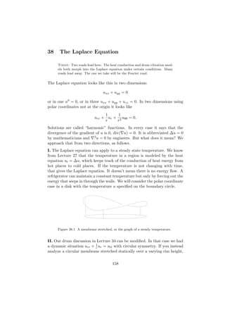
not steam:
dV
heat added = 717 dT + 287 T [Joule/kg]
V
is supposed to hold whenever a process occurs that makes a small change
in the temperature T [Kelvin] and the specific volume V [m3 /kg] of the
gas. Here, the pressure comes in, again for air, through the ideal gas law
P = 287ρT , V = 1/ρ. A main point discovered: that expression is not a
differential. This was so important that they even made a special symbol
for the heat added: d Q which survives to this day in some books.
/
156](https://image.slidesharecdn.com/dn-120926135951-phpapp02/85/Dn-162-320.jpg)
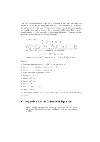
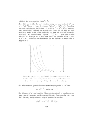
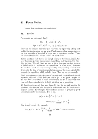
![Fourier
M. Fourier observed the examples we’ve seen. He felt that something is
missing. Of course you probably feel too that our boundary conditions are
somewhat artificial, made to fit the product solutions we found. Fourier
wondered if you could work with some such boundary conditions as
u(1, θ) = f (θ) = θ2
or something like that, which has nothing to do with the cosines and sines.
It is an interesting question to ask. Could it be possible that you could
somehow expand f in terms of cosines and sines?
Could a function f (θ) which is not expressed in terms of the cos(nθ) and
sin(nθ) actually have those hidden within it?
The question is more strange too, because it is nearly the opposite of what
we are used to, like
θ2 θ4
cos(θ) = 1 − + − ···
2 24
That goes the wrong way–we wanted θ2 in terms of trig functions. Eventu-
ally we will achieve this on page 168. But if the answer to the question is
yes, then you can solve the membrane problem by just putting in the powers
of r as we did above:
If f (θ) = c0 + a1 cos(θ) + b1 sin(θ) + a2 cos(2θ) + b2 sin(2θ) + · · ·
then you can solve the BVP as follows, assuming convergence:
u(r, θ) = c0 + r a1 cos(θ) + b1 sin(θ) + r2 a2 cos(2θ) + b2 sin(2θ) + · · ·
Fourier wanted to know how to extract the frequencies hidden in all func-
tions.
1
0.5
0
-0.5
-1
0 10 20 30 40 50 60
Figure 39.1 What frequencies could be hidden in this function? It is plotted
on the interval [0, 10π].
162](https://image.slidesharecdn.com/dn-120926135951-phpapp02/85/Dn-168-320.jpg)
![Problems
1. We need to check carefully that when u is a solution to the Laplace equation, then
so is 6u, or cu for any constant c. How can that be checked? Start with the first order
derivative
∂u
∂r
Is it true that ∂cu = c ∂u ? Then how about the second derivatives, say (cu)θθ ? Is that
∂r ∂r
the same as c(uθθ )? That is the essential idea behind the fact that
2 2
(cu) = c u
Why does that prove what we need?
2. We also need to know that a sum of harmonic functions is harmonic. Reason that out
similarly to Problem 1.
3. We also need to understand that a linear combination of harmonic functions is harmonic.
Part of the calculation goes like this.
2 2 2 2 2
(c1 u1 + c2 u2 ) = (c1 u1 ) + (c2 u2 ) = c1 (u1 ) + c2 (u2 )
Which part of that is by Problem 1? 2? Why does that prove what we need?
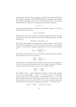
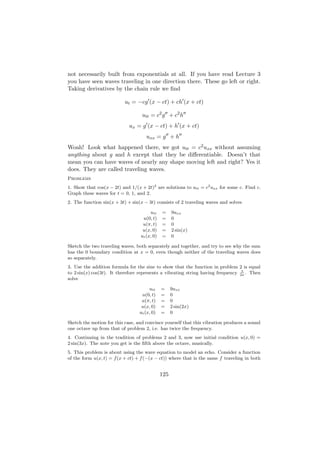
40 Fourier’s Dilemma
Today: We look into pictures to help Fourier find his hidden frequencies.
We now know that it is easy to solve the boundary value problem
1 1
urr + ur + 2 uθθ = 0 (0 < r < 1, 0 ≤ θ ≤ 2π)
r r
with a specified value at the boundary circle u(1, θ) = f (θ) provided that we
can express f (θ) in terms of a series made from our list
cos(nθ), sin(nθ), (n > 0) and also 1.
Fourier wanted to know how to extract the frequencies hidden in f .
1
0.5
0
-0.5
-1
0 10 20 30 40 50 60
Figure 40.1 What frequencies could be hidden in this function on [0, 10π]?
163](https://image.slidesharecdn.com/dn-120926135951-phpapp02/85/Dn-169-320.jpg)
![• On page 39 we proved by an energy argument that our favorite second
order equation y = −y has only those solutions that we know from
calculus.
• There is no choice about Fourier coefficients as shown in Lecture 41.
If a function has a Fourier series, there is only one. But we avoid the
question of when a function has a series. Too advanced.
a Wave Equation example
Here is a case where you can gain a good tool for the toolbox. This is an outline of an
elegant argument which is usually considered to be outside the scope of this course. But
some of you asked about it, and it is a good challenge. This is the wave equation for a
string of length L
utt = uxx
u(0, t) = f (t)
u(L, t) = g(t)
u(x, 0) = h(x)
ut (x, 0) = k(x)
The initial shape h and velocity k are both given, and you can even shake both ends of the
string by f and g. I claim that uniqueness holds: if u1 (x, t) and u2 (x, t) are solutions, then
they are identically equal. How can this be proved? Let w be the difference, w = u2 − u1 .
You’ll need to convince yourself that subtracting wipes out all the boundary and initial
conditions so that w solves the problem
wtt = wxx
with
w(0, t) = w(L, t) = w(x, 0) = wt (x, 0) = 0
Once we prove that w = 0 then we will have u1 = u2 like we claim.
RL` 2 2
´
New idea: Let E = 0 1 wt + 1 wx dx which we call the energy of the string. In a
2 2
nutshell here is what happens:
i) The energy is conserved i.e. constant in time.
ii) E starts out being 0 at t = 0.
iii) The only way E can be identically 0 is if w is identically 0.
Of those items only i) needs a calculation, and the others just need some careful thinking.
Here is the calculation without any explanatory comments:
Z L Z L
dE
= (wt wtt + wx wxt ) dx = (wt wxx + wx wxt ) dx
dt 0 0
Z L
= (wt wx )x dx = [wt wx ]L = 0
x=0
0
Problem Fill in as many details of this argument as you can.
169](https://image.slidesharecdn.com/dn-120926135951-phpapp02/85/Dn-175-320.jpg)
![43 selected answers and hints
page 4
3. A function increases where the derivative is positive, so y is increasing on (−1, 0) and
(1, ∞).
4. If y(0) = 1/2 then y decreases as long as it is positive, so probably y → 0.
5. y = (.03 + .005t)y
page 7
1. −kx−2 = mx , the minus because the force acts toward the large mass at the origin,
the k as a generic constant, and m the small mass. Or, if you know the physics better,
k = mM G where M is the large mass and G the gravity constant. G is about 10−10 [mks].
page 11
2. On a left face of one of these, yx > 0. The equation tells you then yt > 0. So these
waves must move left.
3. The idea here is to find the derivatives. This is not strictly necessary because we
already proved that waves traveling right at speed 3 are solutions no matter what shape
they are. But it helps to check specific cases when you are learning something new.
5. You can tell the velocity of the (model of the) dune, because that is how we interpret
our solutions. But looking at the derivation of the model, we never connected the wind
speed specifically with the dune speed. So you can’t tell how fast the wind is. It is not
part of the model.
Naturally the real wind is going the same way as the real dunes, but not at the same
speed.
page 14
1. Yes, because z (t) = y (t − 3) by the chain rule, and because y(a − y) evaluated at t is
equal to z(a−z) evaluated at t−3. The point here is that no explicit t occurs in the logistic
equation. This time translation does not occur with an equation such as x = xt − x2 .
3. Here is one way to outline the arithmetic. Write x = e−at1 as suggested. Starting with
y = a(1 + c1 e−at )−1 you have in years 1800, 1820, and 1840:
5.3(1 + c1 ) = a
9.6(1 + c1 x) = a
2
17(1 + c1 x ) = a
The first and second expressions are both a, so they are equal, and this will give you x
in terms of c1 . Similarly the first and third give you x2 in terms of c1 . Consequently c1
solves a quadratic equation, which you can solve. Then it is easy to get a, x, and t1 in
that order.
page 17
p
2. x(t) = −1/ t + 1/9
170](https://image.slidesharecdn.com/dn-120926135951-phpapp02/85/Dn-176-320.jpg)
![page 125
3. sin(x+3t)+sin(x−3t) = sin(x) cos(3t)+cos(x) sin(3t)+sin(x) cos(3t)−cos(x) sin(3t) =
2 sin(x) cos(3t) has the initial condition 2 sin(x) of problem 2. For this problem the only
difference is that we want 2 sin(2x) instead, so the solution is 2 sin(2x) cos((2)(3t)). You
have to multiply the 3t by 2 because otherwise you would not be creating traveling waves
which are functions of x ± 3t, as required by the wave equation utt = 32 uxx .
8. We have said only that sums of left and right traveling waves are solutions. In this
case the function is seen to be a solution to utt = uxx by differentiating it, or by using the
idea of problem 3 to write it as a sum of left and right traveling waves: cos(t) sin(x) =
(1/2)(sin(x + t) + sin(x − t)).
page 129
q
3. cos(kn2 t) sin(nx) where k = EI
ρ
, n = 1, 2, 3...
4. the answer is not unique because of insufficient BC
page 135
1
2. x = 2
works, so s is no more than 2.
page 140
3. The radius of convergence is no affected by the −10, so it is 1, just like in Problem
1. But when x = 8.3, |x − 10| > 1 so you are outside the radius of convergence. You are
trying to add powers of 1.7, which diverges.
page 148
16
1. J0 (4) = s6 (4) + E = 1 − 9
+ E = −7 + E
9
“ ”
48 410 48 42 44
2. The tail E = 22 42 62 82
− 22 42 62 82 102
+ ··· = 22 42 62 82
1− 102
+ 102 122
− ··· If you
48 2
remember about alternating series, that is less than 22 42 62 82
= 3
.
7 2
So J0 (4) < − 9 + 3
< 0 as needed.
page 157
` ´
1. Integrating 717 dT
T
+ 287 dV
V
= dS you find ln T 717 V 287 = S + c
page 164
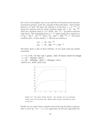
1. In the figure there seem to be at least two frequencies at work. The larger one has 10
cycles in the interval [0, 10π] and seems to start positively at θ = 0. So a multiple of cos(θ)
is a good guess for that one. The smaller one is harder to count. It has less amplitude
and about 4 cycles for each of the larger ones. It is probably cos or sin of 4θ or 5θ, with
a smaller amplitude than the other one.
page 167
3. We know about the product solutions cos(nt) sin(nx) for the wave equation with these
string boundary conditions. And we know that you can form linear combinations of these
solutions. So the idea: If we could write f as a series of sines, then we could use those
177](https://image.slidesharecdn.com/dn-120926135951-phpapp02/85/Dn-183-320.jpg)

This document provides an introduction to ordinary differential equations. It begins with an example of the "banker's equation" which models the growth of a bank account balance over time. It then introduces the concept of slope fields, which provide a graphical representation of the behavior of solutions to a differential equation. The document emphasizes reading and understanding differential equations through examples rather than providing a comprehensive textbook.