This thesis develops mathematical models to analyze the population dynamics of Ateles Hybridus (Brown Spider Monkeys) in fragmented and non-fragmented landscapes. It begins with a single-patch model and analyzes the equilibria and stability. It then integrates this into a multi-patch model accounting for migration between patches. Various parameters are explored, including survival rates, birth gender probability, and reproduction rate. The goal is to provide insights into the endangerment of this species and potential solutions based on modeling their population structure and environment.

![1 Introduction
Mathematical modeling is a branch of mathematics studying the behavior of systems and
maps in a current state using past events. We want to know how to generate mathematical
representations or models, how to validate them, how to use them, and how and when their
use is limited. Since the modeling of devices and phenomena is essential to both engineering
and science, engineers and scientists have very practical reasons for doing mathematical
modeling. In addition, engineers, scientists, and mathematicians want to experience the
sheer joy of formulating and solving mathematical problems.
Definition 1.0.1. A Mathematical Model is a representation in mathematical terms
of the behavior of real devices and objects [3].
In this study, we create a mathematical model to estimate the dynamics of Ateles
Hybridus, also known as the Brown Spider Monkey, in a non-fragmented and fragmented
landscape. The Brown Spider Monkeys (of several species) live in the tropical rain forests
of Central and South America and occur as far north as Mexico. They have long, lanky
arms and prehensile (gripping) tails that enable them to move gracefully from branch
to branch and tree to tree. These nimble monkeys spend most of their time aloft, and
maintain a powerful grip on branches even though they have no thumbs [4].
Ateles Hybridus are a social species and gather in groups of up to two or three dozen
animals. At night, the groups split up into smaller sleeping parties of a half dozen or fewer.
Foraging also occurs in smaller groups, and is usually most intense early in the day. Spider
monkeys find food in the treetops and feast on nuts, fruits, leaves, bird eggs, and spiders.
They can be noisy animals and often communicate with many calls, screeches, barks, and
other sounds.
Typically, females give birth to only a single baby every one to five years. The var-
iegated spider monkey gives birth to single young, after a gestation of 225 days. Baby
spider monkeys tend to cling to their mother’s belly for around the first four months of
life, after which they climb to her back, eventually developing enough independence to
travel on their own. Young monkeys depend completely on their mothers for about ten
1](https://image.slidesharecdn.com/9d3d2085-f7a6-4c7e-b969-d5a81244a5d5-150502091715-conversion-gate02/85/Thesis-2015-5-320.jpg)
![This is the well known Fibonacci equation and a prime example of a difference equation.
Since we consider an initial population of Ateles Hybridus of under 1,000 inhabitants, a
discrete time-scale is most sufficient.
2.2 Basic Ideas of Difference Equations
The idea of a difference equation can now be formulated in a general way, applicable to a
wide variety of biological problems. Difference equations arise in problems like the previous
example.
Definition 2.2.1. Let a rule express a recursive sequence, where members of a sequence
are in terms of previous members of a sequence. If the rule defines the kth member of the
sequence in terms of the (k-1)st member (and possibly also the number k itself), then it is
said to be a first-order difference equation [1].
Once a value is specified for y1, the difference equation then determines the rest of the
sequence uniquely. The value given for y1 is called an initial condition and the sequence
obtained is called a solution of the difference equation.
Definition 2.2.2. An Initial Condition of a system is a set of starting-point values
belonging to or imposed upon the variables in an equation that has one or more arbitrary
constants. [1].
In our model of Ateles Hybridus, we use biological data [5] to best give realistic
initial conditions for our patch populations to be tested under various survival and birth
probabilities. In this way, we do not have an unbalance in our population that would be
deemed unrealistic in real life.
Definition 2.2.3. Let a rule express a member of a sequence in terms of previous members
of a sequence. If the rule defines the kth member of the sequence in terms of the (k-2)th
member (and possibly also the (k-1)st member or the number k itself), then it is said to be
a second-order difference equation [1].
4](https://image.slidesharecdn.com/9d3d2085-f7a6-4c7e-b969-d5a81244a5d5-150502091715-conversion-gate02/85/Thesis-2015-8-320.jpg)
![A unique solution for second order difference equations is determined once the initial
values of both y1 and y2 are specified. Difference equations of third and higher orders
may be defined in a similar way. This process of repeatedly substituting old values back
into the difference equation to produce new ones is known as iteration. It is clear that
this process will eventually produce yk for any prescribed value of k. For some difference
equations it is possible to find a simple formula giving the solution yk as a function of k.
Such a formula is said to provide a ‘closed-form’ solution of the difference equation and
enables values for large times, such as y100, to be calculated directly, without the need to
calculate all the preceding members of the sequence.
2.3 Fixed Points and Stability
In the applications of difference equations to biological systems, a solution represents some
quantity measured at equal intervals of time.
Definition 2.3.1. A solution in which the measured values do not change with time is
called a constant or steady-state solution [1].
Definition 2.3.2. An orbit is a collection of points related by the evolution function of
the dynamical system. The orbit is a subset of the phase space and the set of all orbits is
a partition of the phase space, that is, different orbits do not intersect in the phase space
[1].
Although a solution chosen at random is unlikely to be automatically in a steady-state,
it may approach a steady-state solution over a long period of time.
Definition 2.3.3. Let f : I → I. A fixed point is a point x such that f(x) = x [1].
Obviously, the orbit of a fixed point is the constant sequence x0, x0, x0, . . . . Fixed points
have the advantage of a simple graphical interpretation, which often provides information
about fixed points even in cases where we cannot solve equations explicitly. A number k
is a fixed point of a function f if and only if the point (k, f(k)) is a point of intersection of
the graphs of y = f(x) and y = x [3].
5](https://image.slidesharecdn.com/9d3d2085-f7a6-4c7e-b969-d5a81244a5d5-150502091715-conversion-gate02/85/Thesis-2015-9-320.jpg)
![Theorem 2.3.4. If x0 is some fixed point for a function f, then we say that x0 is a source
and is unstable if |f (x0)| > 1. On the other hand, x0 is a sink and is asymptotically stable
if |f (x0)| < 1. If |f (x0)| = 1, this test is inconclusive and other tests must be used. We
note that if |f (x0)| = 1, x0 is called non-hyperbolic.
Proof. See [3].
Definition 2.3.5. A scalar λ is called an Eigenvalue of an n × n Matrix A if there
is a nontrivial solution x of the equation Ax = λx. Such an x is called an eigenvector
corresponding to the eigenvalue λ.
Theorem 2.3.6. Eigenvalue Stability Theorem. If all roots of the characteristic
equation at an equilibrium point satisfy |λ| < 1, then all solutions of the system with
initial values sufficiently close to an equilibrium will approach the equilibrium point as
t → ∞ and the equilibrium point is known as a stable equilibrium point [3].
Theorem 2.3.7. Eigenvalue Instability Theorem. If all roots of the characteristic
equation at an equilibrium point satisfy |λ| ≥ 1, then all solutions of the system with initial
values sufficiently close to an equilibrium will approach the equilibrium as t → −∞ and
the equilibrium point is known as an unstable equilibrium point [3].
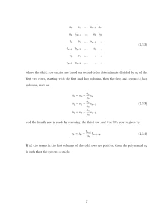
In a discrete-time system, the Jury Criterion [2] can be used to determine its stability.
A system is stable if and only if all roots of the characteristic polynomial
Char(λ) = |A − λI| = (λ) = a0λn
+ a1λn−1
+ · · · + an−1λ + an (2.3.1)
are inside the unit circle. To use the Jury Criterion, we can begin by multiplying our
polynomial a(λ) by −1 if necessary to make a0 positive. Then, form the array
6](https://image.slidesharecdn.com/9d3d2085-f7a6-4c7e-b969-d5a81244a5d5-150502091715-conversion-gate02/85/Thesis-2015-10-320.jpg)
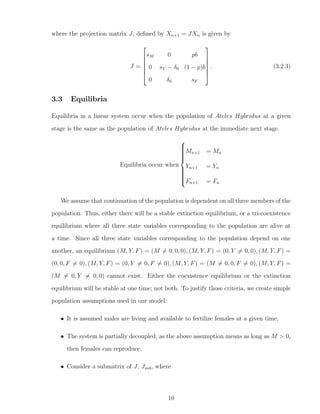
![3 Single-Patch Model
We implement a discrete model to study the population dynamics of Ateles Hybridus in
a single patch. Data [5] suggest that for a population level of under 1,000 inhabitants, a
discrete model is most suitable. Different patches resemble a landscape which has been
fragmented over the past few years. A population is divided into categories by sex: male
and female. Furthermore, the population is broken down so that the female population
is broken into subgroups: adult females and young females, to account for an age of
reproductive ability. Additionally, females are the dispersing sex in spider monkeys. In
our population, a young female acquires its reproductive ability around their seventh year,
at which point they disperse from their group or “family” in search of another group where
they will spend their reproductive life. This activity will require the adult females to select
a target patch other than their original one, and successfully cover the distance between
their current patch and their selected one. An additional hostility factor includes a target
patch that is close to its carrying capacity in which the female could have a considerable
amount of trouble staying alive, hence having to make a second decision. Because of the
given variables in female dispersal throughout the patches in question, we consider three
ecological processes. These are the natural per-capita birth and death rate, the average
time for females to reach reproductive ability, and eventually, a forced migration process
at the time of female adulthood.
3.1 State Variables
A patch is composed of a single group of individuals divided into male and female coun-
terparts, where females are further divided into two subgroups, which are those who have
reached reproductive ability, and those who have not. We assume that the time to reach
reproductive ability is, on average, seven years of age. Each one of these groups is repre-
sented by the variables M, Y, F, where M = Males, Y = Young (Unreproductive) Females
and F = Females. Parameters for the model are estimated from previous studies and
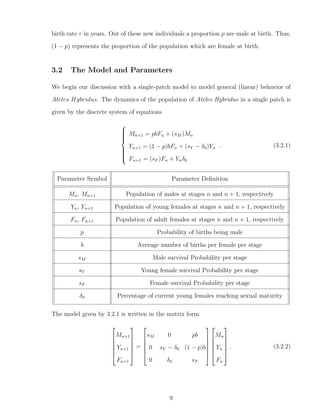
published data [5]. We assume that new individuals are the result of births at a per-capita
8](https://image.slidesharecdn.com/9d3d2085-f7a6-4c7e-b969-d5a81244a5d5-150502091715-conversion-gate02/85/Thesis-2015-12-320.jpg)
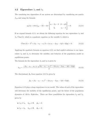
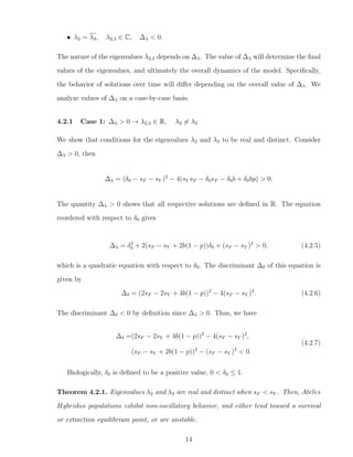
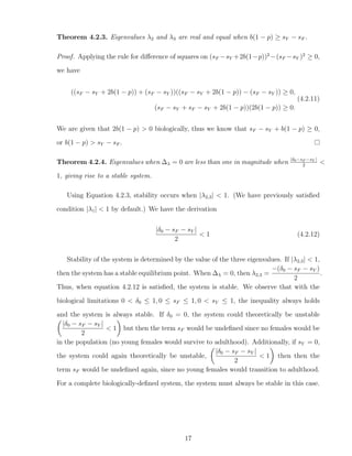
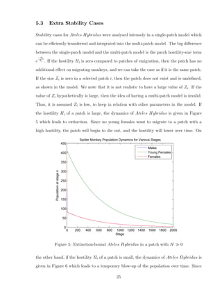
![4.2.3 Case 3: ∆λ < 0 → λ2,3 ∈ C, λ2 = λ3
When we consider ∆λ < 0 for equation 4.2.4. The eigenvalues are defined on C. Eigenval-
ues are complex in this case and the discriminant ∆λ is given as
∆λ = (δ0 − sF − sY )2
− 4(sY sF − δ0sF − δ0b + δ0bp) < 0 (4.2.13)
The equation 4.2.13 in terms of δ0 is written as
δ2
0 + 2(sF − sY + 2b(1 − p))δ0 + (sF − sY )2
< 0. (4.2.14)
Biologically, young females must transition into adult females to give the existence of adult
females, thus δ0 > 0. The only option in this case is that there are two real roots for δ0.
Thus, ∆λ < 0 between the two real roots, therefore we must have ∆δ > 0 Applying the
quadratic formula on 4.2.14 with respect to δ0, two roots of δ0 can be found explicitly
δ01,2 = −(sF − sY + 2b(1 − p)) ± (sF − sY + 2b(1 − p))2 − (sF − sY )2. (4.2.15)
We must have
∆δ =(2sF − 2sY + 4b(1 − p))2
− 4(sF − sY )2
,
(sF − sY + 2b(1 − p))2
− (sF − sY )2
> 0.
We remark that in Equation 4.2.15 another biological condition 0 ≤ p < 1 is imposed. If
in the case that p = 1, then ∆δ = 0, which would be a contradiction since ∆δ > 0. We
then expand the difference of squares:
([sF − sY + 2b(1 − p)] + [sF − sY ])([sF − sY + 2b(1 − p)] − [sF − sY ]) > 0,
[2sF − 2sY + 2b(1 − p)][2b(1 − p)] > 0,
[sF − sY + b(1 − p)][b(1 − p)] > 0.
18](https://image.slidesharecdn.com/9d3d2085-f7a6-4c7e-b969-d5a81244a5d5-150502091715-conversion-gate02/85/Thesis-2015-22-320.jpg)
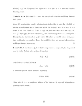
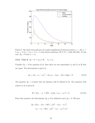
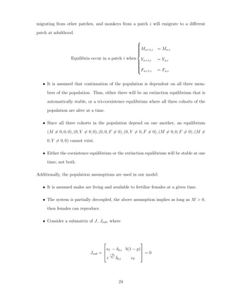
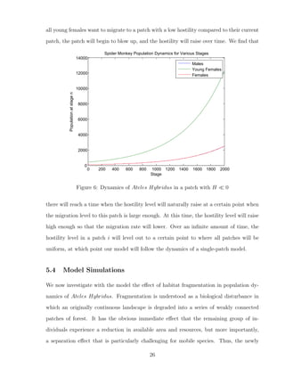
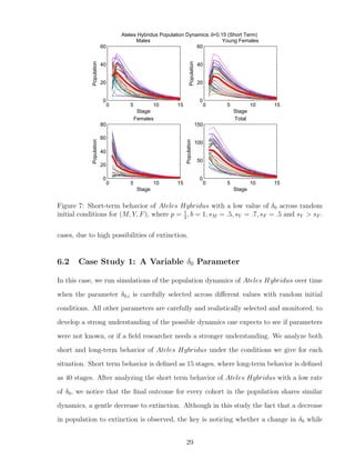
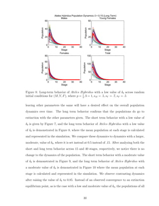
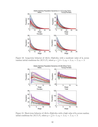
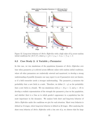
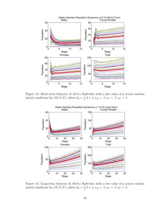
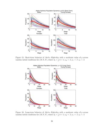
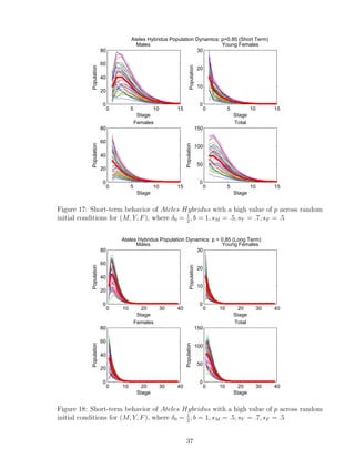
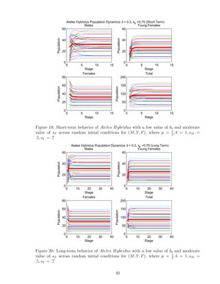
![and running simulations with multiple initial conditions. With this information, we better
understand the dynamics of a single patch. Biologists studying the endangerment of Ateles
Hybridus have observed that young females migrate to a different patch at the time they
reach reproductive capabilities and become part of the female cohort (and hence no longer
part of the young female cohort). We use conclusions given to us by the single-patch model
analysis and apply it to an integrated multi-patch model using the assumption of forced
migration of young females to a new patch, and we create new parameters to account for
differences in patch quality, and determine the dynamics of Ateles Hybridus in a multi-
patch setting. It has been reported for these animals that they tend to segregate in very
conservative female to male ratios when they are in ideal ecological conditions [5]. It is also
important to consider the direction of the path of young females to their target patch at the
time they reach reproductive maturity. We consider that a female which is migrating to its
target patch would move straight to the patch instead of a random pathway. Additionally,
in our multi-patch estimation model, we consider that no females are allowed to stay at
the patch they were born; all females must migrate to a different patch at the time they
reach reproductive maturity. We assume that home patches that have lesser quality will
translate as higher chances of a female reaching their target patch of a higher quality, and
vice versa.
5.1 Multiple Patch Model Diagram and Equations
Given our results from our single-patch model, we can integrate our findings to estimate
behavior in a modified multiple-patch model. Our multi-patch model is similar to the
model for a single-patch, with some changes in definitions of parameters, and extra scalar
parameters added. Mortality rates are different for each group but are equal between
patches. In our multi-patch model, we consider forced migration of a young female to a
new patch at the time they acquire reproductive maturity. We create the restriction on
our parameters Hi and Zi such that −∞ < Hi < ∞ and 0 < Zi. Since Hi represents a
hostility parameter of a given patch, high values of Hi (Hi > 0) correspond to a high level
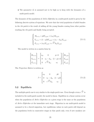
21](https://image.slidesharecdn.com/9d3d2085-f7a6-4c7e-b969-d5a81244a5d5-150502091715-conversion-gate02/85/Thesis-2015-25-320.jpg)

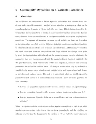
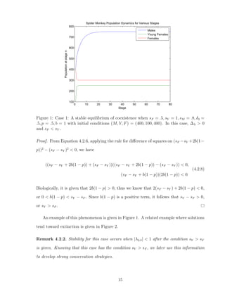
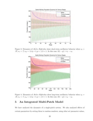
![7 Discussion
The original data given [5] and inspiration of the model is based on biological data that
would accurately represent true population dynamics of Ateles Hybridus. The single-
patch model is created as a accurate starter tool that can be used to further estimate
behavior of Ateles Hybridus in a multi-patch model setting. One of the strongest points
noted during the stability analysis is the fact that a minuscule change in parameters can
have a large impact on the final outcome. Additionally, if ∆λ = 0, then solutions are
always stable. We used the inequality to warrant stable solutions when ∆λ = 0, given by
|δ0 − sF − sY |
2
< 1 (7.0.1)
We see that the equilibrium corresponding to extinction is stable if and only if it is the
only equilibrium. If it is not the only equilibrium, then surviving populations would tend
toward the tri-coexistence survival equilibrium. We had the benefit of the limitations
on certain parameters to make them biologically realistic. These include the probability
coefficients p, sM , sY , sF , δ0, where 0 ≤ p, sM , sF , ≤ 1 and 0 < sY , δ0 ≤ 1. We were able
to exploit these parameter limitations to infer further results on our single-patch model
that can be integrated into our multi-patch model. For the above example, when we were
determining the value of sY − sF , we know it eventually is equal to a number between
−1 and 1. Therefore, it does not matter what parameter values were chosen, just as long
as their respective limitations were called for. Changing the certain values of sY and sF
does not make much of a difference to our model, as long as sY − sF has the same value.
Spider monkeys are an endangered species, and further research can be done in the area
of further integration of our single-patch model into a multi-patch model that strongly
simulates movement of young females to other patches as they reach their reproductive
stage. Some same equilibrium points may be given, but extra parameters in the model
can understandably give further complexities.
We developed a program that analyzes the importance of parameters p, δ0,i alone, and
43](https://image.slidesharecdn.com/9d3d2085-f7a6-4c7e-b969-d5a81244a5d5-150502091715-conversion-gate02/85/Thesis-2015-47-320.jpg)
![References
[1] Adler, R., A. G. Konheim, and M. H. McAndrew. “Topological Entropy.” Transactions
of the American Mathematical Society. 114 (1965): 309-319.
[2] Castillo-Ch´avez, Carlos, and Fred Brauer. Mathematical Models in Population Biol-
ogy and Epidemiology. New York: Springer, 2001.
[3] Caswell, Hal. Matrix Population Models: Construction, Analysis, and interpretation
of matrix population models in the biological sciences. 1989.
[4] Cordovez, J. M., J. R. Arteaga B, M. Marino, A. G. de Luna and A. Link. “Popu-
lation Dynamics of Spider Monkey (Ateles Hybridus) in a Fragmented Landscape in
Colombia.” Biometrics. (2012): 6-8.
[5] G. Cowlishaw and R. Dunbar. “Primate Conservation Biology.” Chicago University
Press. Chicago. 2000.
[6] Doubleday, W. G., “Harvesting in Matrix Population Models” Biometrics. 31 (1975):
189-200.
[7] F. Michalski and C. A. Peres., “Biological Conservation”. p. 383-396. 2005.
[8] C. A. Peres. “Conservation Biology” 15 (2001). p. 1490-1505.
[9] Y. Shimooka, C. Campbell, A. Di Fiore, A. M. Felton, K. Izawa, A. Link, A.
Nishimura, G. Ramos-Fernandez and R. Wallace. “Demography and group composi-
tion of Ateles” p. 329-348. Cambridge University Press. 2008.
47](https://image.slidesharecdn.com/9d3d2085-f7a6-4c7e-b969-d5a81244a5d5-150502091715-conversion-gate02/85/Thesis-2015-51-320.jpg)
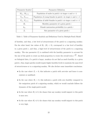
![9 Appendix A
The following program is used to visualize the final dynamics of our model with certain
parameter inputs. The current input corresponds to an unstable system where the pop-
ulations approach infinity as time approaches infinity. Here, we modified our values of
sM , sY , sF , b, p, and δ0 to determine the behavior and overall result of the population dy-
namics of Ateles Hybridus. We were then able to group our results into cases 1, 2, or 3
based on the behavior that is analyzed in our single patch model. In many cases, small
changes in certain parameter values would turn into large changes in the dynamics of the
model.
function nt=ex2p1(t)
sM=.5;
sF=.49;
p=1/3;
b=.75;
muY=0;
deltaN=.1;
A=[ sM 0 p*b; % enter the matrix
0 1-muY-deltaN (1-p)*b;
0 deltaN sF];
n0 = [400 100 400]’; % enter the initial vector
nt=zeros(3,t); % alocate memory for the vectors
nt(:,1)=n0; % set the initial vector as the first one on the array
for j=2:t % the loop
nt(:,j)=A*nt(:,j-1);
end
plot(nt’);
xlabel(’Stage’)
ylabel(’Population at stage n’)
48](https://image.slidesharecdn.com/9d3d2085-f7a6-4c7e-b969-d5a81244a5d5-150502091715-conversion-gate02/85/Thesis-2015-52-320.jpg)

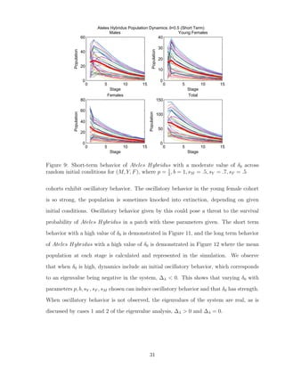
![This is the program that is used to simulate the dynamics of each of the cohorts of the
population of Ateles Hybridus. These are males, young females, and females. We also
included a plot which would graph the total population as well. We created a MATLAB
graph which would generate four subplots displaying each of the cohorts’ dynamics. We
input a value k that would generate the number of stages that would be run in the model,
and input the number of iterations that would be given based on random initial conditions,
and our goal is to see whether random initial conditions had strength within the model.
We did conclude that the parameter p did have strength in the model, and the parameter
δ0 had strength in the model as far as having an influence on the ideal value of sF .
function M1=meanModel2(k)
% Modify J.flores M.Buhr 3/17/2015
% input k=number of simulations of a single state variable
% output the data for the state variable and it graph and the
% graph of the mean.
N=15;
p=.5;
b=1;
mu m=.5;
mu y=.3;
mu f=.5;
delta=.85;
H=1;
A=1;
M1=[];
M2=[];
M3=[];
M4=[];
T end=39;
52](https://image.slidesharecdn.com/9d3d2085-f7a6-4c7e-b969-d5a81244a5d5-150502091715-conversion-gate02/85/Thesis-2015-56-320.jpg)
![for ii=1:k % number of simulations
M=zeros(1,N);
Y=zeros(1,N);
F=zeros(1,N);
Tot=zeros(1,N);
M(1)=randi(50);
Y(1)=randi(30);
F(1)=randi(70);
Tot(1)=M(1)+Y(1)+F(1);
S=1;
for n=2:T end % number of periods
M(n)=p*b*F(n-1)+(1-mu m)*M(n-1);
Y(n)=(1-p)*b*F(n-1)+(1-mu y-delta)*Y(n-1);
F(n)=(1-mu f)*F(n-1)+Y(n-1)*(delta);
Tot(n)=M(n)+Y(n)+F(n);
end
T=1:T end;
M1=[M1;M]; % change M by Y or Mby F to obtain the data for the other state vari-
ables.
M2=[M2;Y];
M3=[M3;F];
M4=[M4;Tot];
end
subplot(2,2,1)
plot(T,M1)
hold on
plot(T,mean(M1),’LineWidth’,3,’Color’,[1 0 0])
53](https://image.slidesharecdn.com/9d3d2085-f7a6-4c7e-b969-d5a81244a5d5-150502091715-conversion-gate02/85/Thesis-2015-57-320.jpg)
![xlabel(’Stage’)
ylabel(’Population’)
title([’Males’])
subplot(2,2,2)
plot(T,M2)
hold on
plot(T,mean(M2),’LineWidth’,3,’Color’,[1 0 0])
xlabel(’Stage’)
ylabel(’Population’)
title([’Young Females’])
subplot(2,2,3)
plot(T,M3)
hold on
plot(T,mean(M3),’LineWidth’,3,’Color’,[1 0 0])
xlabel(’Stage’)
ylabel(’Population’)
title([’Females’])
subplot(2,2,4)
plot(T,M4)
hold on
plot(T,mean(M4),’LineWidth’,3,’Color’,[1 0 0])
xlabel(’Stage’)
ylabel(’Population’)
title([’Total’])
text(-45,397,[’Ateles Hybridus Population Dynamics: delta = ’,num2str(delta),’ (Long
Term)’])
end
54](https://image.slidesharecdn.com/9d3d2085-f7a6-4c7e-b969-d5a81244a5d5-150502091715-conversion-gate02/85/Thesis-2015-58-320.jpg)