Mathematical Modeling HW7 Ch4 Finding a perfect fit model

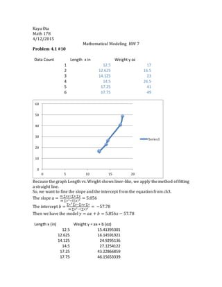
1. Kaya Ota
Math 178
4/12/2015
Mathematical Modeling HW 7
Problem 4.1 #10
Data Count Length x in Weight y oz
1 12.5 17
2 12.625 16.5
3 14.125 23
4 14.5 26.5
5 17.25 41
6 17.75 49
Because the graph Length vs. Weight shows liner-like, we apply the method of fitting
a straight line.
So, we want to fine the slope and the intercept from the equation from ch3.
The slope 𝑎 =
𝑚 ∑𝑥𝑦−∑𝑥 ∑𝑦
𝑚 ∑𝑥2−(∑𝑥)2 = 5.856
The intercept 𝑏 =
∑𝑥2
∑𝑦−∑𝑥𝑦 ∑𝑥
𝑚 ∑𝑥2 −(∑𝑥)2 = −57.78
Then we have the model 𝑦 = 𝑎𝑥 + 𝑏 = 5.856𝑥 − 57.78
Length x (in) Weight y = ax + b (oz)
12.5 15.41395301
12.625 16.14591921
14.125 24.9295136
14.5 27.1254122
17.25 43.22866859
17.75 46.15653339
0
10
20
30
40
50
60
0 5 10 15 20
Series1

2. Then the model fits to the data points
Problem 4.3 #3
X Y 1st divided diff 2nd divided diff 3rd divided diff
0 7 8 5 0
1 15 18 5 0
2 33 28 5 0
3 61 38 5 0
4 99 48 5 0
5 147 58 5 0
6 205 68 0 0
7 273 0 0 0
From the divided difference table, we can know it shows quadratic polynomials
Problem 4.3 #6
x y 1st divided diff
46 40 3.333333333
49 50 2.5
51 55 8
52 63 4.5
54 72 -1
56 70 7
57 77 -4
58 73 17
59 90 3
60 93 3
61 96 -8
62 88 11
0
10
20
30
40
50
60
0 5 10 15 20
Data
Model

3. 63 99 11
64 110 1.5
66 113 7
67 120 7
68 127 3.333333333
71 137 -5
72 132 0
Negative numbers in the columns of the 1st divided diff makes invalid to model with
the lower-polynomials. The graph is the original data of x vs. y
Problem 4.3 #7
x y 1st divided diff
17 19 3
19 25 7
20 32 9.5
22 51 6
23 57 7
25 71 11.66666667
31 141 -18
32 123 64
33 187 1.666666667
36 192 13
37 205 47
38 252 -4
39 248 23
41 294 0
0
20
40
60
80
100
120
140
160
0 20 40 60 80
Series1

4. Because the 1st divided diff contains negative value, it tells the invalid of identifying
the lower-polynomials.
However, the graph x vs. y looks like the lower-order polynomials, so we could
apply the n-th divided difference manually.
Problem 4.4 #1(b)
0
50
100
150
200
250
300
350
0 10 20 30 40 50
Series1