The document provides an introduction to statistics, emphasizing its two main branches: descriptive and inferential statistics. It explains the definitions, classifications, stages of statistical investigation, and basic terms, such as population, sample, and variable types. The document also discusses the applications of statistics in various fields while highlighting its limitations concerning qualitative characteristics and the need for skilled interpretation.


![Arba Minch University Department of Statistics
College of Natural Sciences Probability and Statistics for Engineers
79
The probability of occurrence of at least one of the two events A and B is given by:
P (A )
(
)
(
)
(
) B
A
P
B
P
A
P
B
If A and B are mutually exclusive events, then
P (A )
(
)
(
) B
P
A
P
B
Conditional Probability and Independence
Let there be two events A and B. Then the probability of event A given that the outcome of event B is
given by: P [A|B] =
]
[
]
[
B
P
AnB
P
Where: P [A |B] is interpreted as the probability of event A on the
condition that event B has occurred. In this case P [A n B] is the joint probability of event A and B, and
P [B] is not equal to zero.
And 0
P(A)
where
,
)
(
)
(
)
/
(
A
P
A
B
P
A
B
P
Example 5.12:120 employees of a certain factory are given a performance test and are divided in to two
groups as those with good performance (G) and those with poor performance (P), then the result is
given below
Good performance (G) Poor performance(P) Total
Male (M) 60 25 80
Female (F) 25 15 40
Total 85 35 120
The probability of a person to be male given that it has a good performance is
P (M|G) =
)
(G
P
G
M
P
=
120
/
85
120
/
60
=
17
12
The probability of a person to be female given that it has a poor performance is
P (F|P) =
)
(P
P
P
M
P
=
120
/
35
120
/
15
=
7
3](https://image.slidesharecdn.com/probabilityandstatistics-4-220924013521-58a533b5/75/probability-and-statistics-4-pdf-79-2048.jpg)


![Arba Minch University Department of Statistics
College of Natural Sciences Probability and Statistics for Engineers
83
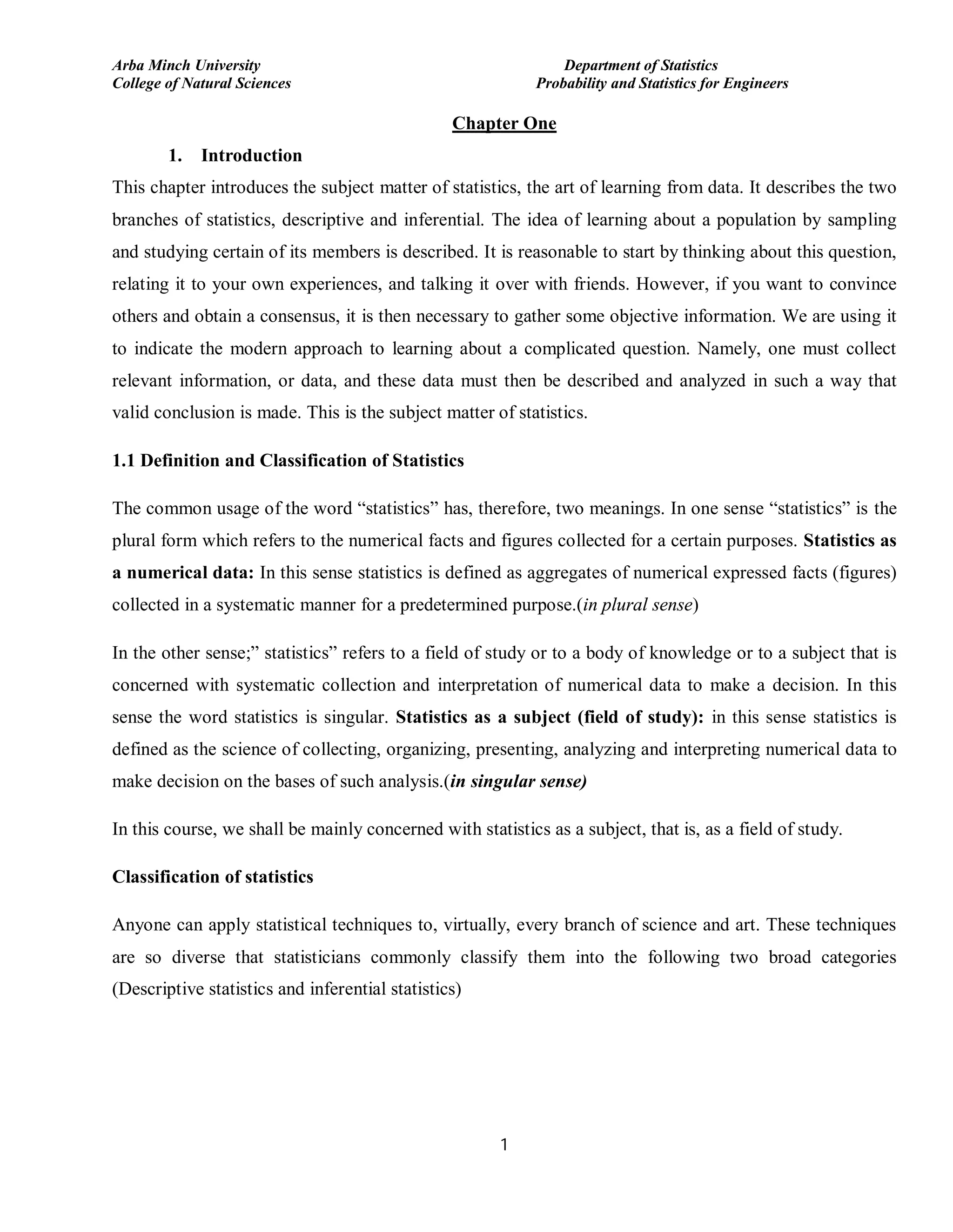
Variance of a Random Variable
Let X be given random variable with expected value (mean) of E(x), then the variance of X is given by:
continous
is
X
if
)
(
)
)
(
(
discrete
is
X
if
)
(
))
(
(
))
(
(
)
(
2
2
dx
x
f
X
E
x
x
X
P
X
E
x
X
E
x
E
X
Var
x
In the form of expectation variance of X is Var(X ) E(X 2
)−[E(X )]2
or
Var(X) = E(X(X-1)) + E(X) – (E(X))2
Where:
( ) = ( = ) ,
= ( = ),
Example 1: Compute the mean and variance of the random variable X, which denotes the number
showing up when a single die is rolled.
Solution: First we have to find the frequency distribution,
X=xi 1 2 3 4 5 6
P(X=xi) 1/6 1/6 1/6 1/6 1/6 1/6
( ) = 1
1
6
+ 2
1
6
+ 3
1
6
+ 4
1
6
+ 5
1
6
+ 6
1
6
= 3.5
( ) = (1 − 3.5)
1
6
+ (2 − 3.5)
1
6
+ (3 − 3.5)
1
6
+ (4 − 3.5)
1
6
+ (5 − 3.5)
1
6
+ (6 − 3.5)
1
6
= 2.9167
Example 2: Compute the mean and variance of the following probability distribution.
( ) =
[0,4],
0 ℎ .
( ) = ( )
=
1
4
=
1
4
1
2
4
0
=
1
4
1
2
4 −
1
2
0 = 2](https://image.slidesharecdn.com/probabilityandstatistics-4-220924013521-58a533b5/75/probability-and-statistics-4-pdf-83-2048.jpg)


![Arba Minch University Department of Statistics
College of Natural Sciences Probability and Statistics for Engineers
86
= 1 – {P(X = 0) + P(X = 1) + P(X = 2)}
P(X = 0) =
0
10
(0.25)0
(0.75)10
= 0.0563
P(X = 1) =
1
10
(0.25)1
(0.75)9
= 0.1877
P(X = 2) =
2
10
(0.25)2
(0.75)8
= 0.2816
.’. P(X >= 3) = 1 – (0.0563 + 0.1877 + 0.2816) = 0.4744
The mean = np = 2.5. The variance = npq = 1.875
Example 2: Suppose that a population of size N = 500 consists of 300 dominants and 200 recessive. For
a sample of size n = 10, calculate the probabilities:-
a) Exactly 2 individuals will be recessive.
b) At least 2 individuals will be recessive.
c) At most 1 individual will be recessive.(Exercise)
d) At most 5 individuals will be recessive.(Exercise)
Let X = recessive, p = probability of recessives = 200/500 = 2/5.
a) P[X=2] = 1210
.
0
5
/
3
5
/
2
2
10 8
2
b) P[X ]
1
[
]
0
[
1
]
2
X
P
X
P , but P[X=0] = 006047
.
0
0
10 10
q
P[X=1] = 040320
.
0
1
10 9
pq .
Hence, P[X2] = 1 - (0.006047 + 0.040320) = 0.9536
Mean = np = 4 V(X) = npq = 12/5
The binomial distribution approaches normal distribution as the number of trials n tends to large (n→ )
for any fixed value of p. A rule of thumb is that for p < 0.5, the normal approximation is adequate if np](https://image.slidesharecdn.com/probabilityandstatistics-4-220924013521-58a533b5/75/probability-and-statistics-4-pdf-86-2048.jpg)
![Arba Minch University Department of Statistics
College of Natural Sciences Probability and Statistics for Engineers
87
>5. Departures from the given conditions result in less accurate approximations. When n is very large
and p is very small (n→∞ &p→0) the binomial distribution approaches Poisson distribution.
iii. Poison Distribution
The Poisson distribution is also used to represent the probability distribution of a discrete random
variable. It is employed in describing random events that occur rarely over a continuum of time or space,
such as number of car accident in certain road corr-section, number of errors in digital communication,
number of type fill errors, etc. The Poisson distribution bears a close similarity to the binomial
distribution. Suppose that we are interested in the number of occurrences of an event E in a time period
of length t. This time period can be split into n equal intervals, each of length t/n. These n intervals can
be treated as n trials by Bernoulli process. But there is difficult. Since the event occurs at various points
of time, it can occur twice or more in one of the trials of length t/n. In case of binomial distribution the
event is dichotomous, and hence there is no possibility of such multiple occurrences within a single trial.
In order to overcome this difficulty we make n larger and larger. When n is large, the trials are shorter in
terms of length of time. As a result, the probability of occurrence of an event in a single trial would be
smaller. It is equivalent of saying that it is a rare event. The binomial distribution can still be used to
represent the distribution of such random events. However, the computations become tedious since n is
very large. This can be explained by example.
Suppose that the number of insects caught in a trap is being studied and that the data are collected on the
number of insects caught per hour. Assume that the probability that an insect will be caught in any
single minute is 0.06. Assume further that the events of insects being trapped are mutually independent
and the probability p = 0.06 remains same for all the minutes. We may use the binomial distribution to
calculate the number of insects caught per hour by considering each minute as a separate Bernoulli trial.
If x is the number of insects caught in a minute then we have: P[X=x] = x
x
x
60
94
.
0
06
.
0
60
Instead of dividing the hour into minutes the seconds may be used as basic units. Then the value of p
would be reduced to, p=0.06/60=0.001. Considering each second as a Bernoulli trial, we would have a
sample size 60 60=3600 for a period of one hour. The binomial distribution would now be:
P[X=x] = x
x
x
3600
999
.
0
001
.
0
3600](https://image.slidesharecdn.com/probabilityandstatistics-4-220924013521-58a533b5/75/probability-and-statistics-4-pdf-87-2048.jpg)
![Arba Minch University Department of Statistics
College of Natural Sciences Probability and Statistics for Engineers
88
Thus when n becomes larger and larger the computations using binomial become tedious. Fortunately, it
has been shown by Poisson that the value of x
n
x
q
p
x
n
approaches the value of
!
x
e
np p
n
X
, when n
becomes large and p becomes small in such a way that the equality, np = is maintained.
The probability mass function of Poisson distribution is given by:
P[X=x] =
!
x
e x
. Where, = np = mean number of times an event occurs.
x = the number of times an event occur. e = Naperian base = 2.7182…
The value of e
can be obtained directly from mathematical tables. In case of Poisson distribution the
counts of alternative events, i.e., failures are not of interest. This is a contrast between binomial and
Poisson distributions. For Poisson distribution all that we need is np, the mean number of successes. We
need not know about n and p individually. Thus, the Poisson distribution is determined by the parameter
.
The special property of Poisson distribution is that its mean and variance are same to .
i.e. In magnitude; mean = variance = .
Example 3:In Black Lion Hospital, the average new born female baby in every 24 hour is 7. What is the
probability that
i. No female babies are born in a day?
ii. Only three female babies are born per day?
iii. Two female babies are born in 12 hours?
In this case = 7 per day
No female baby born in a day P(X = 0) =
!
0
70
7
e
= e-7
= 0.0138189
Only three female babies are born P(X = 3) =
!
3
73
7
e
= 0.78998
Two female babies are born in 12 hours → in this case = 7⁄2 = 3.5
P(X = 2) =
!
2
)
5
.
3
( 2
5
.
3
e
= 0.184959](https://image.slidesharecdn.com/probabilityandstatistics-4-220924013521-58a533b5/75/probability-and-statistics-4-pdf-88-2048.jpg)
![Arba Minch University Department of Statistics
College of Natural Sciences Probability and Statistics for Engineers
89
Example 4: In some experiments it was observed that the incidence of stem fly in black gram was 6
percent. Suppose we examine 50 black gram plants in a field at random. What is probability that at most
3 plants will be found to be affected by stem fly?
The probability that a plant is affected by stem fly is given as 0.06. The number of plants observed (n =
50). Hence, = np = 3. The required probability is
P[X 3] = P[X = 0] + P[X = 1] + P[X = 2] + P[X = 3]
P[X = x] =
!
x
e x
P[X = 0] =
!
0
30
3
e
= e-3
P[X = 1] =
!
1
31
3
e
= 3e-3
P[X = 2] =
!
2
32
3
e
= 4.5e-3
P[X = 3] = 3
3
3
3
5
.
4
6
27
!
3
3
e
e
e
P[X 3
] = 13e-3
. From mathematical table it can found that e-3 =
0.0498.
Therefore P[X3] = 13 0498
.
0
= 0.6474.
Common Continuous Probability Distributions
i. Normal Distribution
The most important and widely used probability distribution is normal distribution. It is also known as
Gaussian distribution. Most of the distributions occurring in practice, for instance, binomial, Poisson,
etc., can be approximated by normal distribution. Further, many of the sampling distributions like
Student’s t, F, & χ2
distributions tend to normality for large samples. Therefore, the normal distribution
finds an important place in statistical inference.
The normal distribution is used to represent the probability distribution of a continuous random variable
like life expectancies of some product, the volume of shipping container, etc.](https://image.slidesharecdn.com/probabilityandstatistics-4-220924013521-58a533b5/75/probability-and-statistics-4-pdf-89-2048.jpg)

![Arba Minch University Department of Statistics
College of Natural Sciences Probability and Statistics for Engineers
91
iii) Find the probability that any student score between 60 & 93. i.e. P[ 60< X < 93]
Solution: Where X is mark of student
ia) Z = 8
.
0
15
72
60
S
X
X
ib) Z = 4
.
1
15
72
93
ic) Z = 0
iia) X = X + ZS = 72 + -1(15) = 57
iib) X = X + ZS = 72 + 1.6(15) = 96
iii) P [60 X 93] = P [
S
X
S
X
X
S
X
93
60
] = P [-0.8 4
.
1
Z ] =
P [-0.8 4192
.
0
2881
.
0
]
4
.
1
0
[
]
8
.
0
0
[
]
4
.
1
0
[
]
0
Z
P
Z
P
Z
P
Z = 0.7073 (This
is from standard normal table).
Example. P(0<Z<1.24)= 0.3925
From the table of Normal curves it can be seen that 68.26% of the area lies within the range of
,
95.46% within the range of
2
, and 99.74% within the range of
3 . This is an important
property of normal distribution which is frequently used in statistical inference.](https://image.slidesharecdn.com/probabilityandstatistics-4-220924013521-58a533b5/75/probability-and-statistics-4-pdf-91-2048.jpg)


![Arba Minch University Department of Statistics
College of Natural Sciences Probability and Statistics for Engineers
100
This table gives the sampling distribution of . If we draw just one sample of three framers from the
population of five farmers, we may draw any one of the 10 possible farmers. Hence, the sample mean
can assume any of the values listed above with the corresponding probabilities. For example, the
probability of the mean 81.67 is ( = 81.67) = 0.2 . Therefore, the sample average, , is a random
variable that depends on which sample is selected. The value varies from 76.00 to 85 which are lower or
higher than the population mean = 80.6 . The average of the estimates of all possible samples for any
sample size is the true population value. That is, the expected value of , denoted by [ ], taken over
all possible samples equals population mean, i.e., [ ] = , in which [ ] =
∑
∑
= = 80.6.
If ~ ( , ), then sample mean ~ ( , / ).
ii. Sampling Distribution of Sample Proportion
Let P represent the proportion of elements in a large population having some characteristic; that is, the
proportion of ‘successes,’ where success corresponds to having that characteristic. If simple random
samples of size n are taken from a population where the proportion of ‘successes’ is p, then the sampling
distribution of ̂ has the following properties:
1. = : The average of all the possible ̂ values is equal to the parameter p. in other words, ̂ is
an unbiased estimator of p.
2. =
( )
: The standard deviation for ̂ decreases as the sample size n increases. For a fixed
sample size, the maximum standard deviation is attained at p=0.5.
3. ̂~ ,
( )
: If n is “sufficiently” large, the distribution of ̂ eventually looks like a normal
distribution with mean p and variance
( )
. The necessary size depends on the value of the
population proportion. It must be large enough that ≥ 5 (1 − ) ≥ 5.
Example: If the population proportion of people who favor a certain issue is 0.3, the sampling
distribution of ̂, when the sample size is 400, is approximately normal with a mean of 0.3 and
standard deviation of
( )
=
. ( . )
=0.023.](https://image.slidesharecdn.com/probabilityandstatistics-4-220924013521-58a533b5/75/probability-and-statistics-4-pdf-100-2048.jpg)