Downloaded 234 times

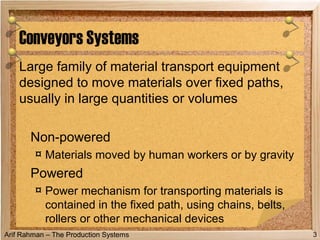
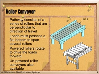
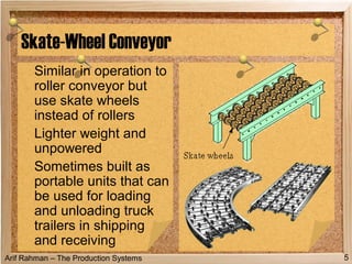
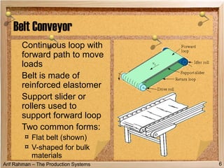
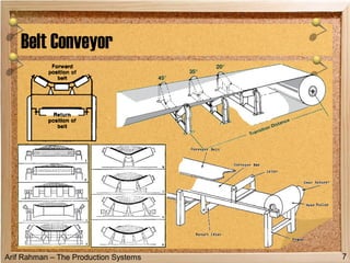
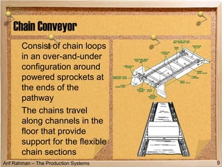
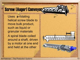
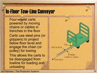
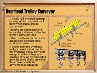
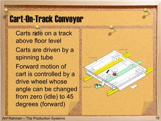
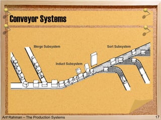
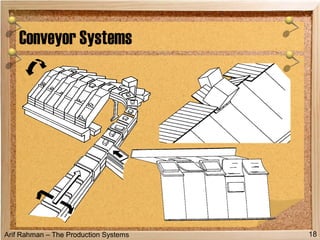
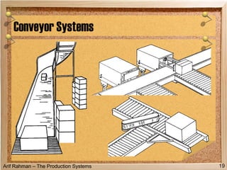
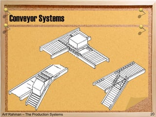

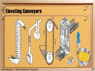
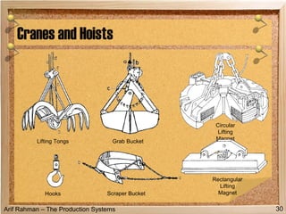
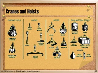
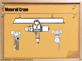
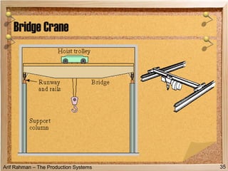
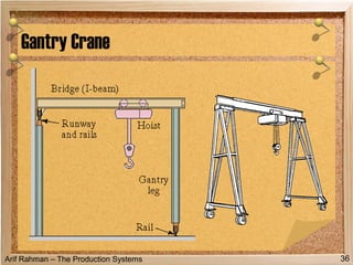
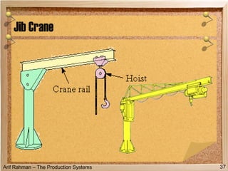
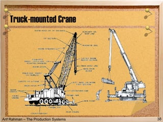
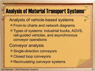
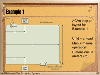
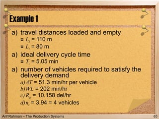
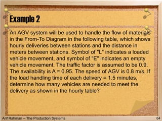
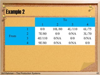


This document discusses different types of material handling equipment used in production systems, including various conveyor types and cranes/hoists. It provides descriptions and diagrams of common conveyor types like roller conveyors, belt conveyors, chain conveyors, and screw conveyors. It also covers analysis of material transport systems using from-to charts, network diagrams, and equations to calculate cycle times.


![[Deck] What's New in Spark-Iceberg Integration via DSV2.pptx](https://cdn.slidesharecdn.com/ss_thumbnails/deckwhatsnewinspark-icebergintegrationviadsv2-260210005337-25955b12-thumbnail.jpg?width=640&height=640&fit=bounds)


