Downloaded 16 times


![Uji Asumsi Klasik: normality
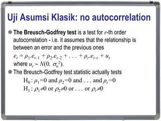
The Bera Jarque normality test
Bera and Jarque testing the residuals for normality by testing
whether the coefficient of skewness and the coefficient of
excess kurtosis are jointly zero.
It can be proved that the coefficients of skewness and
kurtosis can be expressed respectively as:
and
The Bera Jarque test statistic is given by
61
b
E u
1
3
2 3 2
[ ]
/
b
E u
2
4
2 2
[ ]
2
~
24
3
6
2
2
2
2
1
b
b
T
W](https://image.slidesharecdn.com/sinf202012-210811091020/85/Modul-Ajar-Statistika-Inferensia-ke-12-Uji-Asumsi-Klasik-pada-Regresi-Linier-Berganda-61-320.jpg)


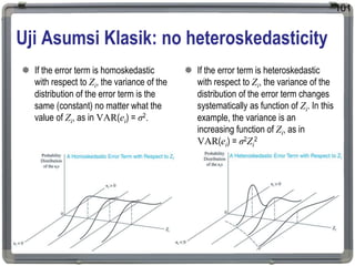


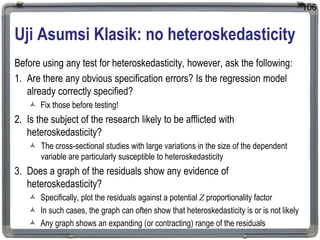


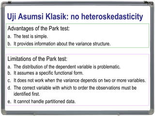


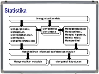
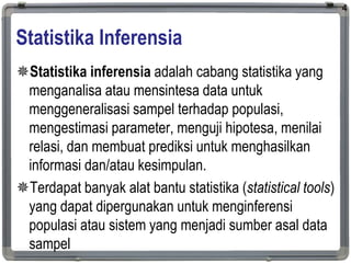
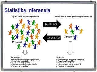
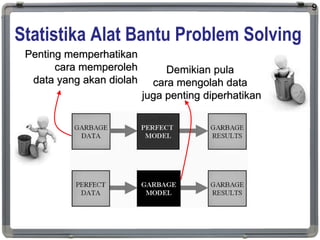
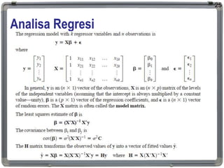
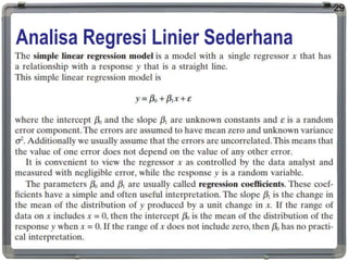
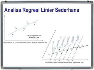
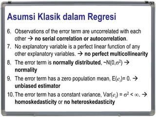
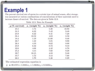
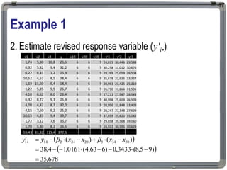
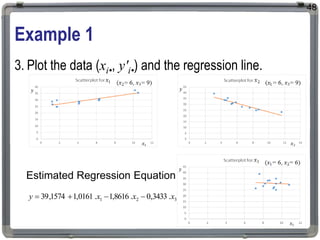
1. The document discusses statistical analysis methods, including regression analysis and classical assumptions for regression models. 2. It explains the differences between correlation and regression, and covers simple and multiple linear regression analysis. 3. Key classical assumptions discussed include the assumptions of linearity, no multicollinearity, normality of residuals, homoscedasticity, and that covariates are uncorrelated with residuals. Methods for testing some of these assumptions are also presented.


