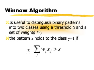
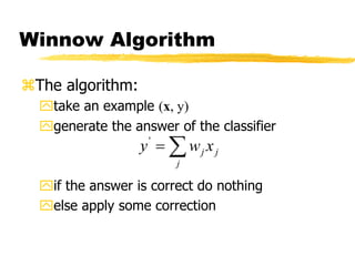
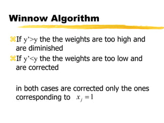
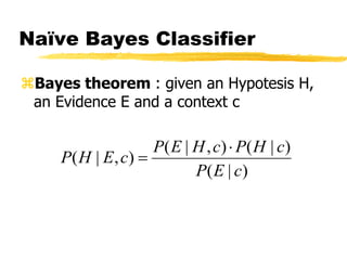
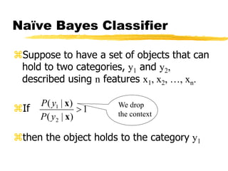
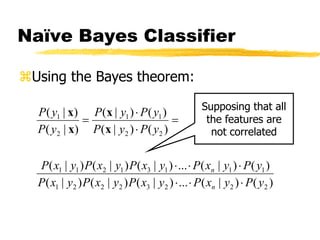
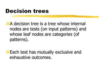
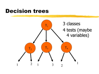
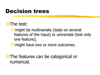
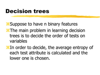
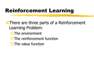
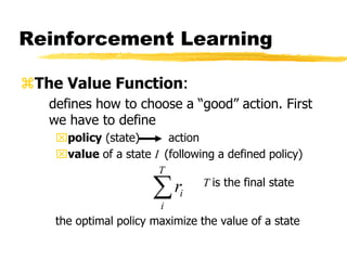
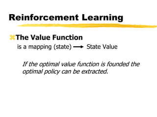
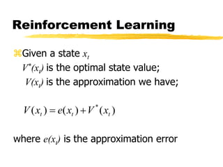
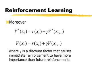
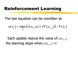
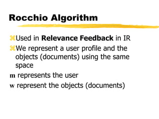
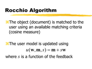
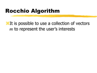
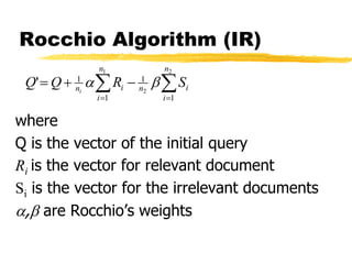
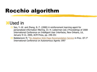
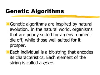
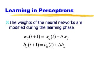
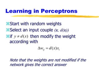
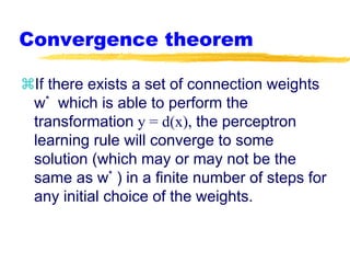
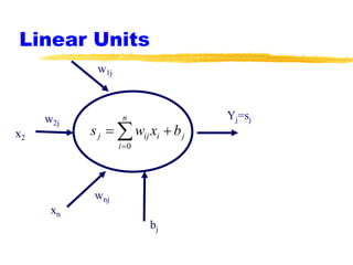
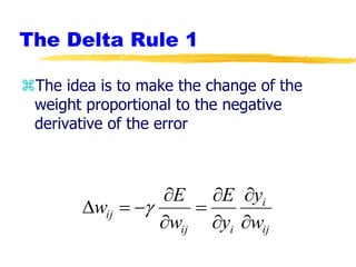
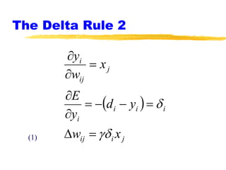
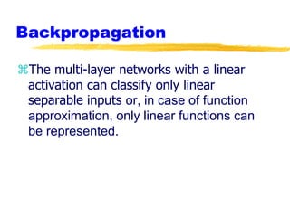
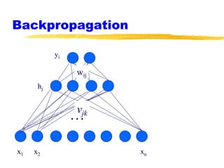
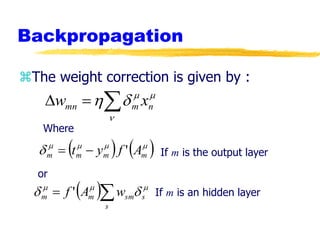
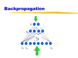
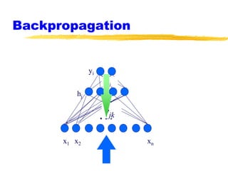
Machine learning and neural networks are discussed. Machine learning investigates how knowledge is acquired through experience. A machine learning model includes what is learned (the domain), who is learning (the computer program), and the information source. Techniques discussed include k-nearest neighbors algorithm, Winnow algorithm, naive Bayes classifier, decision trees, and reinforcement learning. Reinforcement learning involves an agent interacting with an environment to optimize outcomes through trial and error.

1. Machine Learning and
Neural Networks

2. Definitions
Machine learning investigates the
mechanisms by which knowledge is
acquired through experience
Machine Learning is the field that
concentrates on induction algorithms and
on other algorithms that can be said to
``learn.''

3. Model
A model of learning is fundamental in any
machine learning application:
 who is learning (a computer program)
 what is learned (a domain)
 from what the learner is learning (the
information source)

4. A domain
Concept learning is one of the most studied
domain: the learner will try to come up with a
rule useful to separate positive examples
from negative examples.

5. The information source
 examples: the learner is given positive
and negative examples
 queries: the learner gets information
about the domain by asking questions
 experimentation: the learner may get
information by actively experiment with
the domain

6. Other component of the
model are
 the prior knowledge
of the learner about the domain. For example the learner may
know that the unknown concept can be represented in a certain
way
 the performance criteria
that defines how we know that the learner has learned
something and how it can demonstrate it. Performance criteria
can include:
 off line or on line measures
 descriptive or predictive output
 accuracy
 efficiency

7. What techniques we will see
kNN algorithm
Winnow algorithm
Naïve Bayes classifier
Decision trees
Reinforcement learning (Rocchio algorithm)
Genetic algorithm

8. k-NN algorithm
The definition of k-nearest neighbors is
trivial:
Suppose that each esperience can be
represented as a point in an space For a
particular point in question, find the k points
in the population that are nearest to the point
in question. The class of the majority of the
of these neighbors is the class to the selected
point.

9. k-NN algorithm
c2
c
c1 c4
c3
c4
c1
c2
c2
c3
c4
1
New input
Inputs already classified
Class 1

10. k-NN algorithm
Finding the k-nearest neighbors reliably
and efficiently can be difficult. Other
metrics that the Euclidean can be used.
The implicit assumption in using any k-
nearest neighbors technique is that items
with similar attributes tend to cluster
together.

11. k-NN algorithm
The k-nearest neighbors method is most
frequently used to tentatively classify
points when firm class bounds are not
established.
The learning is done using only positive
examples not negative.

12. k-NN algorithm
Used in
 Schwab, I., Pohl, W., and Koychev, I. (2000) Learning to recommend from
positive evidence. In: H. Lieberman (ed.) Proceedings of 2000 International
Conference on Intelligent User Interfaces, New Orleans, LA, January 9-12, 2000,
ACM Press, pp. 241-247

13. Winnow Algorithm
Is useful to distinguish binary patterns
into two classes using a threshold S and a
set of weights
the pattern x holds to the class y=1 if
j
w
s
x
w
j
j
j 

(1)

14. Winnow Algorithm
The algorithm:
take an example (x, y)
generate the answer of the classifier
if the answer is correct do nothing
else apply some correction


j
j
j x
w
y'

15. Winnow Algorithm
If y’>y the the weights are too high and
are diminished
If y’<y the the weights are too low and
are corrected
in both cases are corrected only the ones
corresponding to 1

j
x

16. Winnow Algorithm application
Used in
 M.J. Pazzani “ A framework for Collaborative, Content Based and Demographic
Filtering” Artificial Intelligence Review, Dec 1999
 R.Armstrong, D. Freitag, T. Joachims, and T. Mitchell " WebWatcher: A Learning
Apprentice for the World Wide Web " 1995.

17. Naïve Bayes Classifier
Bayes theorem : given an Hypotesis H,
an Evidence E and a context c
)
|
(
)
|
(
)
,
|
(
)
,
|
(
c
E
P
c
H
P
c
H
E
P
c
E
H
P



18. Naïve Bayes Classifier
Suppose to have a set of objects that can
hold to two categories, y1 and y2,
described using n features x1, x2, …, xn.
If
then the object holds to the category y1
1
)
|
(
)
|
(
2
1

x
x
y
P
y
P We drop
the context

19. Naïve Bayes Classifier
)
(
)
|
(
...
)
|
(
)
|
(
)
|
(
)
(
)
|
(
...
)
|
(
)
|
(
)
|
(
)
(
)
|
(
)
(
)
|
(
)
|
(
)
|
(
2
2
2
3
2
2
2
1
1
1
1
3
1
2
1
1
2
2
1
1
2
1
y
P
y
x
P
y
x
P
y
x
P
y
x
P
y
P
y
x
P
y
x
P
y
x
P
y
x
P
y
P
y
P
y
P
y
P
y
P
y
P
n
n










x
x
x
x
Using the Bayes theorem:
Supposing that all
the features are
not correlated

20. Naïve Bayes Classifier
Used in:
 Mladenic, D. (2001) Using text learning to help Web browsing. In: M. Smith, G.
Salvendy, D. Harris and R. J. Koubek (eds.) Usability evaluation and interface
design. Vol. 1, (Proceedings of 9th International Conference on Human-
Computer Interaction, HCI International'2001, New Orleans, LA, August 8-10,
2001) Mahwah, NJ: Lawrence Erlbaum Associates, pp. 893-897.
 Schwab, I., Pohl, W., and Koychev, I. (2000) Learning to recommend from
positive evidence. In: H. Lieberman (ed.) Proceedings of 2000 International
Conference on Intelligent User Interfaces, New Orleans, LA, January 9-12, 2000,
ACM Press, pp. 241-247, also available at .Self, J. (1986) The application of
machine learning to student modelling. Instr. Science, Instructional Science 14,
327-338.

21. Naïve Bayes Classifier
 Bueno D., David A. A. (2001) METIORE: A Personalized Information Retrieval
System. In M. Bauer, P. J. Gmytrasiewicz and J. Vassileva (eds.) User Modeling
2001. Lecture Notes on Artificial Intelligence, Vol. 2109, (Proceedings of 8th
International Conference on User Modeling, UM 2001, Sonthofen, Germany, July
13-17, 2001) Berlin: Springer-Verlag, pp. 188-198.
 Frasconi P., Soda G., Vullo A., Text Categorization for Multi-page Documents: A
HybridNaive Bayes HMM Approach, ACM JCDL’01, June 24-28, 2001

22. Decision trees
A decision tree is a tree whose internal
nodes are tests (on input patterns) and
whose leaf nodes are categories (of
patterns).
Each test has mutually exclusive and
exhaustive outcomes.

23. Decision trees
T1
T3
T2
T4
1 2 1 3 2
1
3 classes
4 tests (maybe
4 variables)

24. Decision trees
The test:
might be multivariate (tests on several
features of the input) or univariate (test only
one feature);
might have two or more outcomes.
The features can be categorical or
numerical.

25. Decision trees
Suppose to have n binary features
The main problem in learning decision
trees is to decide the order of tests on
variables
In order to decide, the average entropy of
each test attribute is calculated and the
lower one is chosen.

26. Decision trees
If we have binary patterns and a set of
pattern  it is possible to write the
entropy as
were p(i|) is the probability that a random
pattern from  belongs to the class i
)
|
(
log
)
|
(
)
( 2 



  i
p
i
p
H
i

27. Decision trees
We will approximate the probability p(i|)
using the number of patterns in 
belonging to the class i divided by the
total number of pattern in 

28. Decision trees
If a test T have k
outcomes, k subsets 1,
2, ...k, are considered
with n1, n2, …, nk patterns.
It is possible to calculate:
T
1
... ...
J
K
)
|
(
log
)
|
(
)
( 2 j
j
i
j i
p
i
p
H 



 

29. Decision trees
The average entropy over all the j
again we evaluate p(j ) has the number of patterns in
 that outcomes j divided by the total number of
patterns in 
  )
(
)
(
)
( j
j
j
j
T H
p
H
E 



 

30. Decision trees
We calculate the average entropy for all
the test T and chose the lower one.
We write the part of the tree and go head
in order to chose again the test that gives
the lower entropy

31. Decision trees
The knowledge in the tree is strongly
dependent from the examples

32. Reinforcement Learning
 An agent tries to optimize its interaction
with a dynamic environment using trial
and error.
The agent can make an action u that
applied to the environment changes its
state from x to x’. The agent receives a
reinforcement r.

33. Reinforcement Learning
There are three parts of a Reinforcement
Learning Problem:
The environment
The reinforcement function
The value function

34. Reinforcement Learning
The environment
at least partially observable by means of
sensors or symbolic description. The theory is
based on an environment that shows its
“true” state.

35. Reinforcement Learning
The reinforcement function
a mapping from the couple (state, action) to
the reinforcement value. There are three
classes of reinforcement functions:
Pure delayed reward: the reinforcements are
all zero except for the terminal state (games,
inverted pendulum)
Minimum time to goal: cause an agent to
perform actions that generate the shortest path to
a goal state

36. Reinforcement Learning
Minimization: the reinforcement is a function of
of limited resources and the agent have to achieve
the goal while minimizing the energy used

37. Reinforcement Learning
The Value Function:
defines how to choose a “good” action. First
we have to define
policy (state) action
value of a state I (following a defined policy)
the optimal policy maximize the value of a state

T
i
i
r T is the final state

38. Reinforcement Learning
The Value Function
is a mapping (state) State Value
If the optimal value function is founded the
optimal policy can be extracted.

39. Reinforcement Learning
Given a state xt
V*(xt) is the optimal state value;
V(xt) is the approximation we have;
where e(xt) is the approximation error
)
(
)
(
)
( *
t
t
t x
V
x
e
x
V 


40. Reinforcement Learning
Moreover
where  is a discount factor that causes
immediate reinforcement to have more
importance than future reinforcements
)
(
)
(
)
( 1
*
*


 t
t
t x
V
x
r
x
V 
)
(
)
(
)
( 1


 t
t
t x
V
x
r
x
V 

41. Reinforcement Learning
We can find
that gives
(**)
 
)
(
)
(
)
(
)
(
)
(
)
(
)
(
)
(
)
(
)
(
1
1
*
*
1
*
1
*












t
t
t
t
t
t
t
t
t
t
x
e
x
V
x
r
x
V
x
e
x
V
x
e
x
r
x
V
x
e



)
(
)
( 1

 t
t x
e
x
e 

42. Reinforcement Learning
The learning process goal is to find an
approximation V(xt) that makes the
equation (**) true for all the state.
The finale state T of a process has a value that is
defined a priori so e(T)=0, so e(T-1)=0 it the (**) is true
and then backwards to the initial state.

43. Reinforcement Learning
Assuming that the function approximator for the
V* is a look-up table (a table with an
approximate state value w for each state) then
it is possible to sweep through the state space
and update the values in the table according to:
  )
(
)
(
)
,
(
max 1 t
t
t
u
x
V
x
V
u
x
r
w 


 


44. Reinforcement Learning
where u is the action performed that
causes the transition to the state xt+1. This
must be done by using some kind of
simulation in order to evaluate  
)
(
max 1

t
u
x
V

45. Reinforcement Learning
The last equation can be rewritten as
Each update reduce the value of e(xt+1)
the learning stops when e(xt+1)=0
  )
(
)
(
)
,
(
max
)
( 1 t
t
t
u
t x
V
x
V
u
x
r
x
e 

 


46. Rocchio Algorithm
Used in Relevance Feedback in IR
We represent a user profile and the
objects (documents) using the same
space
m represents the user
w represent the objects (documents)

47. Rocchio Algorithm
The object (document) is matched to the
user using an available matching criteria
(cosine measure)
The user model is updated using
where s is a function of the feedback
w
m
m
w s
s
u 

)
,
,
(

48. Rocchio Algorithm
It is possible to use a collection of vectors
m to represent the user’s interests

49. Rocchio and Reiforcement
Learning
The goal is to have the “best” user’s
profile
The state is defined by the weight vector
of the user profile

50. Rocchio Algorithm (IR)
where
Q is the vector of the initial query
Ri is the vector for relevant document
Si is the vector for the irrelevant documents
, are Rocchio’s weights

 




2
2
1
1
1
1
1
'
n
i
i
n
n
i
i
n S
R
Q
Q i



51. Rocchio algorithm
Used in
 Seo, Y.-W. and Zhang, B.-T. (2000) A reinforcement learning agent for
personalized information filtering. In: H. Lieberman (ed.) Proceedings of 2000
International Conference on Intelligent User Interfaces, New Orleans, LA,
January 9-12, 2000, ACM Press, pp. 248-251
 Balabanovic M. “An Adaptive Web Page Recomandation Service in Proc. Of 1th
International Conference on Autonomous Agents 1997

52. Genetic Algorithms
Genetic algorithms are inspired by natural
evolution. In the natural world, organisms
that are poorly suited for an environment
die off, while those well-suited for it
prosper.
Each individual is a bit-string that encodes
its characteristics. Each element of the
string is called a gene.

53. Genetic Algorithms
Genetic algorithms search the space of
individuals for good candidates.
The "goodness" of an individual is
measured by some fitness function.
Search takes place in parallel, with many
individuals in each generation.

54. Genetic Algorithms
The algorithm consists of looping through
generations. In each generation, a subset
of the population is selected to reproduce;
usually this is a random selection in which
the probability of choice is proportional to
fitness.

55. Genetic Algorithms
Reproduction occurs by randomly pairing
all of the individuals in the selection pool,
and then generating two new individuals
by performing crossover, in which the
initial n bits (where n is random) of the
parents are exchanged. There is a small
chance that one of the genes in the
resulting individuals will mutate to a new
value.

56. Neural Networks
An artificial network consists of a pool of
simple processing units which
communicate by sending signals to each
other over a large number of weighted
connections.

57. Artificial Neuron
x1
x2
xn
w1j
w2j
wnj
j
n
i
i
ij
j b
x
w
s 
 
0
)
( j
j s
f
y 
yj
bj
j
s
e


1
1

58. Neural Networks
Each unit performs a relatively simple job:
receive input from neighbors or external sources
and use this to compute an output signal which
is propagated to other units (Test stage).
Apart from this processing, there is the task of
the adjustment of the weights (Learning stage).
The system is inherently parallel in the sense
that many units can carry out their computations
at the same time.

59. Neural Networks
1. Learning stage
2. Test stage
(working stage)
Your knowledge
is useless !!

60. Classification (connections)
As for this pattern of connections, the main
distinction we can make is between:
Feed-forward networks, where the data flow
from input to output units is strictly feed-forward.
The data processing can extend over multiple
layers of units, but no feedback connections or
connections between units of the same layer are
present.

61. Classification
Recurrent networks that do contain feedback
connections. Contrary to feed-forward networks,
the dynamical properties of the network are
important. In some cases, the activation values
of the units undergo a relaxation process such
that the network will evolve to a stable state in
which these activations do not change anymore.
Classification (connections)

62. Recurrent Networks
In other applications, the change of the
activation values of the output neurons are
significant, such that the dynamical behavior
constitutes the output of the network.

63. Classification (Learning)
We can categorise the learning situations in
two distinct sorts. These are:
Supervised learning in which the network is
trained by providing it with input and matching
output patterns. These input-output pairs are
usually provided by an external teacher.

64. Unsupervised learning in which an (output)
unit is trained to respond to clusters of pattern
within the input. In this paradigm the system is
supposed to discover statistically salient
features of the input population. Unlike the
supervised learning paradigm, there is no a
priori set of categories into which the patterns
are to be classified; rather the system must
develop its own representation of the input
stimuli.
Classification (Learning)

65. Perceptron
A single layer feed-forward network consists of
one or more output neurons, each of which is
connected with a weighting factor wij to all of the
inputs xi.
xi
b
b

66. Perceptron
In the simplest case the network has only two
inputs and a single output. The output of the
neuron is:
suppose that the activation function is a
threshold







 

2
1
i
i
i b
x
w
f
y







0
1
0
1
s
if
s
if
f

67. Perceptron
In this example the simple network (the
neuron) can be used to separate the
inputs in two classes.
The separation between the two classes is
given by
0
2
2
1
1 

 b
x
w
x
w

68. Perceptron
x1
x2
x
x
x
x
x
x
x
x
x

69. Learning in Perceptrons
The weights of the neural networks are
modified during the learning phase
ij
ij
ij
ij
ij
ij
b
t
b
t
b
w
t
w
t
w








)
(
)
1
(
)
(
)
1
(

70. Learning in Perceptrons
Start with random weights
Select an input couple (x, d(x))
if then modify the weight
according with
Note that the weights are not modified if the
network gives the correct answer
i
ij x
x
d
w )
(


)
(x
d
y 

71. Convergence theorem
If there exists a set of connection weights
w* which is able to perform the
transformation y = d(x), the perceptron
learning rule will converge to some
solution (which may or may not be the
same as w* ) in a finite number of steps for
any initial choice of the weights.

72. Linear Units
x2
xn
w1j
w2j
wnj
j
n
i
i
ij
j b
x
w
s 
 
0
bj
Yj=sj

73. The Delta Rule 1
The idea is to make the change of the
weight proportional to the negative
derivative of the error
ij
i
i
ij
ij
w
y
y
E
w
E
w









 

74. The Delta Rule 2
 
j
i
ij
i
i
i
i
j
ij
i
x
w
y
d
y
E
x
w
y













(1)

75. Backpropagation
The multi-layer networks with a linear
activation can classify only linear
separable inputs or, in case of function
approximation, only linear functions can
be represented.

76. Backpropagation
. . .
x1 x2 xn
vjk
hj
wij
yi

77. Backpropagation
When a learning pattern is clamped, the
activation values are propagated to the
output units, and the actual network output
is compared with the desired output
values, we usually end up with an error in
each of the output units. Let's call this
error eo for a particular output unit o. We
have to bring eo to zero.

78. Backpropagation
The simplest method to do this is the
greedy method: we strive to change the
connections in the neural network in such
a way that, next time around, the error eo
will be zero for this particular pattern. We
know from the delta rule that, in order to
reduce an error, we have to adapt its
incoming weights according to the last
equation (1)

79. Backpropagation
In order to adapt the weights from input to
hidden units, we again want to apply the
delta rule. In this case, however, we do
not have a value for for the hidden units.

80. Backpropagation
Calculate the activation of the hidden
units






 

n
k
k
jk
j x
v
f
h
0

81. Backpropagation
And the activation of the output units








 
0
j
j
ij
i h
w
f
y

82. Backpropagation
If we have  pattern to learn the error is
 
2
0
2
1
2
2
1
2
2
1
  
 
























































i j
n
k
jk
ij
i
i j
ij
i
i
i
i
k
j
x
v
f
w
f
t
h
w
f
t
y
t
E

83. Backpropagation
   












j
i
j
i
i
i
ij
ij
h
h
A
f
y
t
w
E
w












.
   




 i
i
i
i A
f
y
t
.



84. Backpropagation
     
 





































i
k
j
ij
i
k
j
i
ij
i
i
i
jk
j
j
jk
jk
x
A
f
w
x
A
f
w
A
f
y
t
v
h
h
E
v
E
v
.
.
.
.

85. Backpropagation
The weight correction is given by :







 n
m
mn x
w
   




 m
m
m
m A
f
y
t '


 

s
s
sm
m
m w
A
f 



 '
Where
If m is the output layer
If m is an hidden layer
or

86. Backpropagation
. . .
x1 x2 xn
vjk
hj
wij
yi

87. Backpropagation
. . .
x1 x2 xn
vjk
hj
wij
yi

88. Recurrent Networks
What happens when we introduce a
cycle? For instance, we can connect a
hidden unit with itself over a weighted
connection, connect hidden units to input
units, or even connect all units with each
other ?

89. Hopfield Network
The Hopfield network consists of a set of
N interconnected neurons which update
their activation values asynchronously and
independently of other neurons.
All neurons are both input and output
neurons. The activation values are binary
(+1, -1)

90. Hopfield Network

91. Hopfield Network
The state of the system is given by the
activation values y = (y k ).
The net input s k (t +1) of a neuron k at
cycle (t +1) is a weighted sum





k
j
k
jk
j b
w
t
y
t
s )
(
)
1
(

92. Hopfield Network
A threshold function is applied to obtain
the output
 
)
1
(
sgn
)
1
( 

 t
s
t
y k
k

93. Hopfield Network
A neuron k in the net is stable at time t
I.e.
A state is state if all the neurons are
stable
 
)
1
(
sgn
)
( 
 t
s
t
y k
k

94. Hopfield Networks
If wjk = wkj the behavior of the system can
be described with an energy function
This kind of network has stable limit points

 


 k
k
k
jk
k
k
j
j y
b
w
y
y
2
1


95. Hopfield net. applications
A primary application of the Hopfield
network is an associative memory.
The states of the system corresponding
with the patterns which are to be stored in
the network are stable.
These states can be seen as `dips' in
energy space.

96. Hopfield Networks
It appears, however, that the network gets
saturated very quickly, and that about
0.15N memories can be stored before
recall errors become severe.

97. Hopfield Networks
Stable
state
State
state
Input

98. Hopfield Networks
Used in
Chung, Y.-M., Pottenger, W. M., and Schatz, B. R. (1998)
Automatic subject indexing using an associative neural network.
In: I. Witten, R. Akscyn and F. M. Shipman III (eds.)
Proceedings of The Third ACM Conference on Digital Libraries
(Digital Libraries '98), Pittsburgh, USA, June 23-26, 1998, ACM
Press, pp. 59-6

99. Self Organization
The unsupervised weight adapting
algorithms are usually based on some
form of global competition between the
neurons.
Applications of self-organizing networks
are:

100. S.O. Applications
clustering: the input data may be
grouped in `clusters' and the data
processing system has to find these
inherent clusters in the input data.

101. S.O. Applications
vector quantisation: this problem occurs
when a continuous space has to be
discretised. The input of the system is the
n-dimensional vector x, the output is a
discrete representation of the input space.
The system has to find optimal
discretisation of the input space.

102. S.O. Applications
dimensionality reduction: the input data
are grouped in a subspace which has
lower dimensionality than the
dimensionality of the data. The system
has to learn an “optimal” mapping.

103. S.O. Applications
feature extraction: the system has to
extract features from the input signal. This
often means a dimensionality reduction as
described above.

104. Self-Organizing Networks
Learning Vector Quantization
Kohonen maps
Principal Components Networks
Adaptive Resonance Theory

105. Kohonen Maps
In the Kohonen network, the output units
are ordered in some fashion, often in a
two-dimensional grid or array, although
this is application-dependent.

106. Kohonen Maps

107. Kohonen Maps
The input x is given to
all the units at the same
time

108. Kohonen Maps
The weights
of the winner unit
are updated
together with the weights of
its neighborhoods

109. Kohonen Maps
Used in:
 Fulantelli, G., Rizzo, R., Arrigo, M., and Corrao, R. (2000) An adaptive open
hypermedia system on the Web. In: P. Brusilovsky, O. Stock and C. Strapparava
(eds.) Adaptive Hypermedia and Adaptive Web-Based Systems. Lecture Notes in
Computer Science, (Proceedings of Adaptive Hypermedia and Adaptive Web-
based Systems, AH2000, Trento, Italy, August 28-30, 2000) Berlin: Springer-
Verlag, pp. 189-201.
 Goren-Bar, D., Kuflik, T., Lev, D., and Shoval, P. (2001) Automating personal
categorizations using artificial neural network. In: M. Bauer, P. J. Gmytrasiewicz
and J. Vassileva (eds.) User Modeling 2001. Lecture Notes on Artificial
Intelligence, Vol. 2109, (Proceedings of 8th International Conference on User
Modeling, UM 2001, Sonthofen, Germany, July 13-17, 2001) Berlin: Springer-
Verlag, pp. 188-198.

110. Kohonen Maps
 Kayama, M. and Okamoto, T. (1999) Hy-SOM: The semantic map framework
applied on an example case of navigation. In: G. Gumming, T. Okamoto and L.
Gomez (eds.) Advanced Research in Computers and Communications in
Education. Frontiers ub Artificial Intelligence and Applications, Vol. 2,
(Proceedings of ICCE'99, 7th International Conference on Computers in
Education, Chiba, Japan, 4-7 November, 1999) Amsterdam: IOS Press, pp. 252-
259.
 Taskaya, T., Contreras, P., Feng, T., and Murtagh, F. (2001) Interactive visual
user interfaces to databases. In: M. Smith, G. Salvendy, D. Harris and R. J.
Koubek (eds.) Usability evaluation and interface design. Vol. 1, (Proceedings of
9th International Conference on Human-Computer Interaction, HCI
International'2001, New Orleans, LA, August 8-10, 2001) Mahwah, NJ: Lawrence
Erlbaum Associates, pp. 913-917.