This document describes a study that introduces a Modified Error Data Normalized Step Size (MEDNSS) algorithm for an adaptive noise canceller. The MEDNSS algorithm uses a time-varying step size that depends on normalization of both the error and data vectors. The performance of the MEDNSS algorithm is analyzed through computer simulation and compared to the Error Data Normalized Step Size algorithm in stationary and non-stationary environments with different noise power levels. Simulation results show the MEDNSS algorithm significantly improves minimizing signal distortion, excess mean square error, and misadjustment factor compared to the EDNSS algorithm.

1. International Association of Scientific Innovation and Research (IASIR)
(An Association Unifying the Sciences, Engineering, and Applied Research)
International Journal of Emerging Technologies in Computational
and Applied Sciences (IJETCAS)
www.iasir.net
IJETCAS 14-555; © 2014, IJETCAS All Rights Reserved Page 152
ISSN (Print): 2279-0047
ISSN (Online): 2279-0055
Modified Error Data Normalized Step Size algorithm Applied to Adaptive
Noise Canceller
1Shelly Garg and 2Ranjit Kaur
1Student, 2Associate Professor, 1,2Department of Electronics and Communication Engineering,
Punjabi University, Patiala, Punjab, INDIA
Abstract: This paper introduces a Modified Error Data Normalized Step Size (MEDNSS) algorithm in which
time varying step size depends upon normalization of both error and data vector. An Adaptive Noise Canceller
(ANC) is used to improve the system performance in the presence of signal leakage components or signal
crosstalk. This ANC consists of three microphones and two adaptive filters that automatically adjust their filter
coefficients by using MEDNSS algorithm. The first adaptive filter cancels the signal leakage components and
second adaptive filter cancels the noise. The performance of the MEDNSS algorithm is analyzed, simulated and
compared to the Error Data Normalized Step Size (EDNSS) algorithm in stationary and non-stationary
environments using different noise power levels. Computer simulation results demonstrate the significant
improvements of the MEDNSS algorithm over the EDNSS algorithm in minimizing the signal distortion, Excess
Mean Square Error (EMSE) and low misadjustment factor.
Keywords: Adaptive filter; Crosstalk reduction; MEDNSS algorithm; Noise cancellation; Stationary and non-stationary
environments.
I. Introduction
An important operation in voice communication systems involves the extraction of unwanted components from
the desired speech signal. This problem arises in many situations, such as helicopters, airplanes and automobiles
where acoustic noise is added to speech signal. Although the single microphone method for noise cancellation
can be achieved using wiener and kalman filtering but two microphone approach using adaptive filtering is a
more powerful technique for this purpose. The strength of the adaptive noise canceller lies in the fact that it
doesn’t require prior knowledge of the speech signal or the corrupted signal. However, a correlation between the
noise that corrupts the speech signal and the noise in the reference input is necessary for the adapting modified
algorithm to remove the noise from the primary input signal. Many two microphone Adaptive Noise
Canceller(ANCs) have been proposed in the literature[1]-[5] using Least mean square(LMS) based algorithms
that changes the step-size of the update equation to improve the tracking ability of the algorithm and its speed of
convergence as well. In all these ANCs, it was assumed that there are no signal leakage components into the
reference input. The presence of these signal leakage components at the reference input is a practical concern
because it causes cancellation of a part of the original speech signal at the input of the ANC, and results in
severe signal distortion and low Signal to Noise Ratio (SNR) at the output of the ANC. The magnitude of this
distortion depends on the signal to noise ratio at the primary and reference inputs. Several techniques were
proposed in the literature to improve the system performance in this case of signal leakage [6], [7]. High
computational complexity is associated with these techniques and algorithms. This paper introduces a Modified
Error Data Normalized Step Size (MEDNSS) where the step size varies according to the error and data vector
normalization and applied to an ANC which consists of three microphones and two adaptive filters.
II. Adaptive Noise Canceller
An adaptive noise canceller with signal leakage in the reference input is shown in the given Figure 1. The
leakage signal is represented as an output of a low pass filter h2 . This conventional ANC consists of two
microphones and one adaptive filter. This adaptive filter is designed by using varying step-size algorithms. First
microphone represents the speech signal S( n ) and the second microphone represents the reference noise
input g( n ) . The signal components leaking from the first microphone through a channel with impulse response
h2 and becomes v2( n ) .An estimate of g( n ) passes through a channel with impulse response h1 becomes
v1( n ) .The combination of S( n )and v1( n ) represented as d( n ) .The combination of g( n ) and v2( n ) represented as
v3( n )which is used as an desired signal of first adaptive filter. These signal components cause distortion in the
recovered speech. So, SNR output decreases as compared to input SNR. It shows that due to signal leakage
components SNR degrades and gives output signal with some distortion.

2. Shelly Garg et al., International Journal of Emerging Technologies in Computational and Applied Sciences, 9(2), June-August, 2014, pp.
152-158
IJETCAS 14-555; © 2014, IJETCAS All Rights Reserved Page 153
Figure 1: Conventional ANC with signal leakage problem [13]
To solve this problem in conventional ANC we introduce a third microphone to provide a signal that is
correlated with the signal components leaked from the primary input. This signal is processed by the first
adaptive filter ( w1 ) to produce a crosstalk free noise at its output. This noisy signal, with almost no leakage
components of the speech, is processed through the second adaptive filter to cancel the noise at its input and
accordingly produces the recovered speech at the output of the ANC.The block diagram of ANC as shown in
Figure2. This ANC consists of three microphones and two adaptive filters. These two adaptive filters are
designed by using varying step size algorithms. First microphone represents the speech signal S( n ) and the
second microphone represents the reference noise input signal g( n ) . The signal components leaking from the
first microphone through a channel with impulse response h3 and becomes v3( n ) .An estimate of g( n ) passes
through a channel with impulse response h1 becomes v1( n ) .The combination of S( n ) and v1( n ) represented as
d( n ) .The combination of g( n ) and v3( n ) represented as d1( n )which is used as an desired signal of first adaptive
filter. These signal components cause distortion in the recovered speech. To solve this problem we introduce a
third microphone to provide a signal v4( n ) , that is correlated with the crosstalk signal that leaks from the
primary microphone into reference one. The transmission path between the third microphone and first adaptive
filter is represented by the impulse response h2 ,and d( n )passes through a channel with impulse response h2
provides v4( n ) signal which is used as the reference noise input signal for 1st adaptive filter. This signal is
processed by the first adaptive filter ( w1 ) to produce a signal without leakage components at the output. This
noisy signal v2( n ) , with almost no leakage components of the speech, is processed through the second adaptive
filter to cancel the noise at its input, and accordingly produces the recovered speech e( n ) at the output of the
ANC.
Figure 2: ANC for solving leakage problem [13]
The performance of ANC may be described in terms of the Excess Mean Square Error (EMSE) or
misadjustment (M).
The EMSE at the nth iteration is defined by

3. Shelly Garg et al., International Journal of Emerging Technologies in Computational and Applied Sciences, 9(2), June-August, 2014, pp.
152-158
IJETCAS 14-555; © 2014, IJETCAS All Rights Reserved Page 154
  


1
0
2
1
1 L
j
e ( n j )
L
EMSE( n ) (1)
Where, e1( n )  e( n )  s( n ) is the excess (residual) error, n is is the iteration number and L is the number of
samples used to estimate the EMSE. The effect of L is just to smooth the plot of EMSE.
The steady state EMSE estimated by averaging EMSE in above equation over n after the algorithm has reached
steady state condition is defined by









1 M 1
n F
EMSE( n )
M F
EMSEss
(2)
Where, M is the total number of samples of the speech signal and F is the number of samples after which the
algorithm reaches steady state condition. The misadjustment (M) is defined as the ratio of the steady state excess
MSE to the minimum MSE.
MSEmin
EMSEss
M  (3)
Where MSEmin equals to the power of the original clean speech signal, S, averaged over samples at which the
algorithm is in steady state is given by









1 M 1 2
n F
S( n )
M F
MSEmin
(4)
III. Modified EDNSS algorithm
Many variable step-size LMS based algorithms have been proposed in the literature[8]-[12] with the aim of
altering the step-size of the update equation to improve the fundamental trade-off between speed of convergence
and minimum Mean Square Error(MSE).A new time-varying step-size was suggested in[10] based on the
estimate of the square of a time-averaged autocorrelation function between e(n) and e(n-1).The step-size is
adjusted based on the energy of the instantaneous error[11]. The performance of this algorithm degrades in the
presence of measurement noise in a system modeling application [10]. The step-size in [12] is assumed to vary
according to the estimated value of the normalized absolute error. The normalization was made with respect to
the desired signal. Most of these algorithms do not perform very well if an abrupt change occurs to the system
impulse response. Based on regularization Newton’s recursion [8], we can write
w( n 1)  w( n )( n )[ ( n )I  RX ]1[ p  RX w( n )] (5)
where : n =iteration number, w =An N×1 vector of adaptive filter weights,  ( n ) =An iteration-dependent
regularization parameter, ( n ) = An iteration dependent step-size, I = The N×N identity
matrix, p( n )  E[ d( n )X( n )] is the cross-correlation vector between the desired signal d(n) and the input signal
x(n) , R ( n ) E[ X( n )X ( n )] T
X  is the autocorrelation matrix of X(n). Writing (5) in the LMS form by replacing p
and RX by their instantaneous approximation d (n) X (n) and X( n )X ( n ) T , respectively, with appropriate
proposed weights, we obtain
w( n ) w( n ) [ e ( n ) I X( n )X ( n )] x( n )e( n ) T
L
2 1
1       (6)
Where:  = A positive constant step size, and  = Positive constants, e( n ) is the system output error
And
  


1
0
2 L 2
i
eL ( n ) e( n i ) (7)
Equation (7) is the squared norm of the error vector, e (n), estimated over its last L values. Now expanding
equation (6) and applying the matrix inversion formula:
1 1 1 1 1 1 [ A BCD]  A  A B[C  DA B]DA (8)
With: A e ( n ) I ,B X( n ),C ,and,D X ( n ) T
 L   
2
We obtain:
X ( n ) e ( n ) X( n )
X ( n ) e ( n )
e ( n ) I e ( n ) IX( n )
[ e ( n ) I X( n )X ( n )]
L
T
L
T
L L
T
L
1 1 2
1 2
1 2 1 2
2 1
  
 
   


 
 
 

 
  (9)
Multiplying both sides of (9) by X (n) from right, and rearranging the equation, we have
2 2
2 1
e ( n ) X( n )
X( n )
[ e ( n ) I X( n )X ( n )] X( n )
L
T
L
 
 

   (10)

4. Shelly Garg et al., International Journal of Emerging Technologies in Computational and Applied Sciences, 9(2), June-August, 2014, pp.
152-158
IJETCAS 14-555; © 2014, IJETCAS All Rights Reserved Page 155
Substituting (12) in (6), we obtain Modified Error Data Normalized Step Size (MEDNSS) algorithm:
X( n )e( n )
e ( n ) ( ) X( n )
( )
w( n ) w( n )
L
2 2
1
1
1
 
 
 

   (11)
Where, is replaced by (1 ) in eq. (11) without loss of generality. The fractional quantity in eq. (10) may be
viewed as a time-varying step-size( n ) of the MEDNSS algorithm. Clearly, ( n ) is controlled by normalization
of both error and input data vectors. This algorithm is dependent on normalization of both data and error. The
parameters  ,L, are appropriately chosen to achieve the best tradeoff between convergence and low final mean
square error. It differs from the NLMS algorithm in the added term 2
eL( n ) with a proportional constant. For
the case when L=n, this added term will increase the denominator of the time -varying step-size ( n ) (the
fractional quantity of (11)), and hence a larger value of  should be used in this algorithm to achieve fast rate
of convergence at the early stages of adaptation. As n increases (with L=n), ( n ) decreases except for possible
up and down variations due to statistical changes in the input signal energy 2
X( n ) . Addition of the parameter
(1 ) improves the system performance as compared to the EDNSS algorithm. To compute (7) with minimal
computational complexity, the error value produced in the first iteration is squared and stored. The error value in
the second iteration is squared and added to the previous stored value. Then, the result is stored in order to be
used in the next iteration and soon. A sudden change in the system response will slightly increase the
denominator of( n ) , but will result in a significantly larger numerator. Thus, the value of step-size will increase
before attempting to converge again. The step-size ( n ) should vary between two predetermined hard limits
[14]. The lower value guarantees the capability of the algorithm to respond to an abrupt change that could
happen at a very large value of iteration number n, while the maximum value maintains the stability of the
algorithm. Note that setting  =0 in this equation results in the standard NLMS algorithm.
IV. Simulations and Results
A comparison of the MEDNSS with EDNSS algorithms are described using Adaptive Noise Cancellation as
shown in Figure 1 and 2 respectively. The simulations are carried out using a male native speech sampled at a
frequency of 11.025 kHz. The number of bits per sample is 8 and the total number of samples is 33000. The
simulation results are presented for stationary and non stationary environments. For the stationary case, the
noise g( n ) was assumed to be zero mean white Gaussian with three different variances as shown in Table1. For
non stationary case, the noise was assumed to be zero mean white Gaussian with variance that increases linearly
from 2
gmin
 =0.00001 to three different maximum values 2
gmax
 such as 0.0001, 0.001, 0.01 as demonstrated in
Table 2. In conventional ANC the following values of parameters were used : N=12, L= 20N,  0.03and
  0.7 ,where N,L,  , and  are the corresponding parameter of the EDNSS algorithm and used in the
adaptive filter(w)shown in Figure 1. ANC in Figure 2 the following values of parameters were used:
N1  N2 12 , L1  L2  20N , 1  0.15,2  0.03,1  0.9,and 2  0.7 where N1 ,L1,1 and 1 are filter length,
error vector length, step size parameter and proportional constant, respectively, of the MEDNSS algorithm as
well as EDNSS algorithm used in the first adaptive filter ( w1 )shown in Fig.2. Similarly, N2 ,L2 ,2 and  2 are
corresponding parameters of the MEDNSS algorithm as well as EDNSS algorithm used in the second adaptive
filter ( w2 ) shown in Fig.2. The value of  were selected as a compromise between fast rate of convergence
and good tracking capability with most concern to have a high rate of convergence in the first adaptive filter and
good tracking capability in the second adaptive filter. The impulse responses of the three autoregressive (AR)
low pass filters used in the simulations are h1 =[1.5 -0.5 0.1], h2 =[2 -1.5 0.3] and h3 =[3 -1.2 0.3].Figure 3
illustrates the performance of conventional ANC for the non-stationary case in which 2
 g max=0.01 as shown in
Table 4. It shows high Excess error. From Top to Bottom, it shows original speech signal S (n), combination of
noise and speech signal d (n), recovered signal e (n) and excess error signal e (n)-S (n). Figure 4 illustrates the
performance of MEDNSS and EDNSS algorithm of an ANC for the non-stationary case in which 2
 g max=0.01 as
shown in Table 3. MEDNSS algorithm provides low EMSE and misadjusment factor as compared to EDNSS
algorithm. The adaptation constants of the algorithm used in both ANCs were selected to achieve a compromise
between small EMSE and high initial rate of convergence for a wide range of noise variances. From these
tables, improvement of up to 34dB in EMSEss using MEDNSS algorithm for ANC as compared to conventional
ANC. It is worthwhile to note that if the noise variance increases, the performance of the conventional ANC
becomes a little better as illustrated in Table 1 and 2. This is expected because increasing noise power level

5. Shelly Garg et al., International Journal of Emerging Technologies in Computational and Applied Sciences, 9(2), June-August, 2014, pp.
152-158
IJETCAS 14-555; © 2014, IJETCAS All Rights Reserved Page 156
results in a less significant effect of the signal leakage at the reference input. This signal leakage provides low
SNR in conventional ANC. So an ANC is used to enhance the SNR rate using MEDNSS and EDNSS algorithm.
Figure 3: Performance of Conventional ANC in non-stationary noise environment ( 2
 gmax =0.01, Table 2)
Figure 4: Performance Comparison between the MEDNSS and EDNSS algorithm of ANC in non-stationary
noise environment ( 2
 g max =0.01, Table 4)
Figure 5: EMSE in dB of the conventional ANC (
2
 g =0.001, Table1), EDNSS algorithm and MEDNSS algorithm using ANC in
stationary noise environment (
2
 g =0.001, Table3)
Table 1: EMSEss and M of the conventional ANC for stationary case
Stationary case Conventional ANC
Gaussian white zero-mean noise, g(n) Steady state EMSE (dB) Misadjustment
(M %)
2
 g =0.0001
-13.6 103.4
2
 g =0.001
-14.68 82.4
2
 g =0.01
-14.94 77.5

6. Shelly Garg et al., International Journal of Emerging Technologies in Computational and Applied Sciences, 9(2), June-August, 2014, pp.
152-158
IJETCAS 14-555; © 2014, IJETCAS All Rights Reserved Page 157
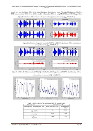
Table 2: EMSEss and M of the conventional ANC for non-stationary case
Non-Stationary Case Conventional ANC
Gaussian Noise g(n)
2
gmin
 =0.00001
Steady State EMSE(dB) Misadjustment
(M %)
2
gmax
 =0.0001
-13.59 105.9
2
gmax
 =0.001
-13.96 97.3
2
gmax
 =0.01
-14.76 80.92
Table 3: Comparison of EDNSS and MEDNSS algorithm of ANC for
Stationary case
Table 4: Comparison of EDNSS and MEDNSS algorithm of ANC for
Non- stationary case
V. Conclusion
In this paper, a new Modified Error Data Normalized Step Size (MEDNSS) Algorithm is proposed to improve
the system performance as compared to EDNSS Algorithm. Computer Simulations, using a new adaptive
algorithm based on normalization of both error and data, show performance superiority of an ANC in decreasing
signal distortion and producing small values of EMSE and Misadjustment factor.
References
[1] S. Ikeda and A. Sugiyama, “An adaptive noise canceller with low signal distortion for speech codecs,” IEEE Trans. On Signal,
Processing, vol. 47, pp 665-674, March 1999.
[2] J. E. Greenberg “Modified LMS algorithms for speech processing with an adaptive noise canceller,” IEEE Trans. On Speech and
Audio Processing, vol. 6, pp 338-351, July 1998.
[3] W.A.Harrison, J S.Lim,and E. Singer, “A new application of adaptive noise cancellation,” IEEE Trans. Acoust.., Speech, Signal
Processing, vol. 34, pp. 21-27, Jan. 1986.
[4] M.J. Al-Kindi and J. Dunlop, “A low distortion adaptive noise cancellation structure for real time applications,” in Proc. IEEE
ICASSP, pp. 2153-2156,1987.
[5] S. F. Boll and D. C. Publisher, “Suppression of acoustic noise in speech using two microphone adaptive noise cancellation,”
IEEE Trans. Acoust.,, Speech, Signal Processing, vol.28, pp. 752-753, 1980.
[6] G. Mirchandani. R. L.Zinser, and J. B.Evans, “A new adaptive noise cancellation scheme in the presence of crosstalk,” IEEE
Trans. Circuits Syst.., vol. 39, pp. 681-694, 1992.
[7] V. Parsa, P. A. Parker, and R. N. Scott,“Performance analysis of a crosstalk resistant adaptive noise canceller,” IEEE Trans.
Circuits Syst., vol. 43, pp. 473-482, 1996.
Stationary Case ANC
Gaussian white zero mean noise
g(n)
EDNSS Algorithm MEDNSS Algorithm
EMSE
steady state
(dB)
M%
EMSE
steady state
(dB)
M%
2
 g =0.0001
-45.14 0.074 -46.6 0.05
2
 g =0.001
-36.75 0.5 -39.36 0.28
2
 g =0.01
-23.24 11.47 -24.9 7.7
Non-Stationary Case ANC
Gaussian Noise g(n)
2
gmin
 =0.00001
EDNSS Algorithm MEDNSS Algorithm
EMSE
steady state
(dB)
M%
EMSE
steady state
(dB)
M%
2
gmax
 =0.0001
-47.67 0.04 -48.12 0.03
2
gmax
 =0.001
-40.51 0.21 -43.09 0.11
2
gmax
 =0.01
-30.10 2.36 -35.6 0.66

7. Shelly Garg et al., International Journal of Emerging Technologies in Computational and Applied Sciences, 9(2), June-August, 2014, pp.
152-158
IJETCAS 14-555; © 2014, IJETCAS All Rights Reserved Page 158
[8] A.H. Sayed, “Fundamentals of Adaptive Filtering.1st Edn.,” Wiley-IEEE Press, Hoboken, NJ, pp: 1168,2003.
[9] S.C. Douglas, and T.H.Y. Meng, “Normalized data nonlinearities for LMS adaptation” IEEE Trans. Signal Processing, vol.42, pp.1352-1365, 1994.
[10] T. Aboulnasr, and K. Mayyas, “A robust variable step-size LMS-type algorithm: Analysis and simulations” IEEE Trans. Signal. Processing vol.45,pp 631-639, 1997.
[11] R.H. Kwong, and E.W. Johnston, “ A variable step-size LMS algorithm”IEEE Trans. Signal Processing vol.40,pp.1633- 1642,1992.
[12] D.W. Kim, H.B. Kang, M.S. Eun and J.S. Choi, “A variable step-size algorithm using normalized absolute estimation error” IEEE Xplore Press, Rio de Janeiro, Brazil, pp: 979-982 ,Aug. 13-16, 1995.
[13] Z.M.Ramadan,“A Three Microphone Adaptive Noise Canceller for Minimizing Reverberation and Signal Distortion”, American Journal of Applied Sciences, vol.5, pp.320-327, 2008.
[14] Z.Ramadan, “Error Vector normalized adaptive algorithm applied to adaptive noise canceller and system identification” American Journal of Applied Sciences, vol.3, pp.710-717, 2010.
Acknowledgment
The main author acknowledges the immense contribution of Dr. Ranjit Kaur (Associate Professor, Department of Electronics and Communication Engineering, Punjabi University, Patiala) for her supervision, encouragement and guidance during the period of this work.