Presentation on life tables . It gives the methods of calculating both the abridged and complete life tables. Fergenecy technique is also included in the presentations. The simple steps make it easier for any student with basic understanding of demography in social statistics and actuarial science to have a grasp of the life table workings and what is required to perform in depth analysis.

1. Week 4: 19 August 2013
Part 2 – Computation of LifeTables II
Lecturer: Salut Muhidin and Bruce Gregor
Department of Marketing and Management
DEM127
Demographic Fundamentals

2. Previously: A Complete (Single Year) Life Table
Life Tables, Australia, 2007–2009: Males
Age lx ndx nqx npx nLx Tx ex
0 100,000 486 0.00486 0.99514 99,586 7,933,720 79.3
1 99,514 40 0.00040 0.99960 99,492 7,834,184 78.7
2 99,474 25 0.00024 0.99976 99,461 7,734,692 77.8
3 99,449 18 0.00018 0.99982 99,440 7,635,231 76.8
4 99,431 14 0.00014 0.99986 99,424 7,535,791 75.8
5 99,417 12 0.00012 0.99988 99,411 7,436,367 74.8
6 99,405 11 0.00011 0.99989 99,400 7,336,956 73.8
7 99,394 10 0.00010 0.99990 99,389 7,237,556 72.8
8 99,384 9 0.00010 0.99990 99,379 7,138,167 71.8
9 99,375 10 0.00009 0.99991 99,370 7,038,788 70.8
10 99,365 9 0.00009 0.99991 99,361 6,939,418 69.8
… … … … … … … …
99 2,090 614 0.29403 0.70597 1,767 5,473 2.6
100+ 1,476 1,476 1.00000 0.00000 3,706 3,706 2.5
2
Numbers
surviving at
exact ages
Deaths
between age x
and x+1
Mean
expectation
of life at
exact age x
Total pop. at
exact aged x and
over
Probability of
living between x
and x+1
Average number
years lived
(living) between x
and x+1
Probability of
dying between
exact ages

3. Other Principles in Computing Life Tables
3
A. Complete vs.Abridged LifeTables
 Life tables with interval more than 1 (n ≠ 1)
B. LifeTable with Death Rates (ASDR = mx)
 Life tables with real-life observed data
 So far, we are assuming that the data input to the Life
Table is hypothetical data (e.g. from some unspecified
sources)
C. Stationary Population:
 Life tables with constant age structure and total pop. size
D. Period vs. Cohort LifeTables

4. A. Complete vs. Abridged Life Tables
4
COMPLETE LIFE TABLE
Values of columns are tabulated for all ages x (single age
group).
ABRIDGED LIFE TABLE
Values of columns tabulated for selected ages x only
(interval age group, e.g. 5 years).
n = no. of years between successive tabulated ages
ndx ‐ the number of deaths between exact ages x and x+n
ndx = lx - lx+n

5. 5
nqx ‐ the probability a person aged exactly x dies before reaching
exact age x+n
x
x
n
x
n
l
d
q  x
n p
1

npx ‐ the probability that a person of exact age x survives to exact
age x+n
nLx ‐ the number of person‐years lived between exact ages x and
x+n ‐‐ the number of persons in a stationary population (with
l0 births) between exact ages x and x+n
nLx = Tx ‐ Tx+n
If deaths are evenly distributed between x and x+n
)
l
l
(
2
n
L n
x
x
x
n 



6. Summary of Abridged Life Tables
6
n
+
x
x
=
x
n l
-
l
d
x
x
n
x
n
l
d
q 
x
n
x
n
x
x
n q
1
l
l
p 

 
n
x
x
x
n T
T
L 


)
l
l
(
2
n
L n
x
x
x
n 


or 1L0 = 0.3l0 + 0.7l1
x
x
x
l
T
e 
Number of dying between exact age (x) and (x+n), can be
estimated by using lx (number of surviving to exact age x).
Probability a person exact aged (x) dies before reaching
exact age (x+n)
Probability a person exact aged (x) survives to exact age
(x+n)
Number of person‐years between age (x) and (x+n ) in
stationary population
(if deaths evenly spread)
For young population between exact age (0) and (1)
Life expectancy at exact age x

7. NOTE: The Final Row in Abridged Life Tables
7
For last row, n= infinity
ndx = lx
nqx = 1.000
nLx = Tx
If ex given  use Lx = Tx = exlx
If ex not given  use
x
x
x
m
l
L

 
Age lx ndx nLx Tx ex
0‐4 100,000 914 497,715 7,705,619 77.06
5‐9 99,086 97 495,187 7,207,904 72.74
●●● ●●● ●●● ●●● ●●● ●●●
65‐69 80,322 7,862 381,954 1,527,270 19.01
70+ 72,460 72,460 1,145,316 1,145,316 15.81
m(x) = mortality / death rates

8. Example: Abridged Life Table
8
Age (x) lx ndx nqx Lx
0 100,000
5 99,428
10 99,246
20 98,838
30 97,974
40 96,775
50 94,136
60 88,670
70 76,738
80 53,816
Source: www.cdc.gov
 The lx column of the abridged life table for white males in the United
States in 2003 is shown below.
• If the value of e80 is 8.00
years (e80 is given).
• Calculate the ndx, nqx, and
Lx columns.
• What is the size (T0) of the
life table population of
white males in the United
States in 2003?

9. Solution
9
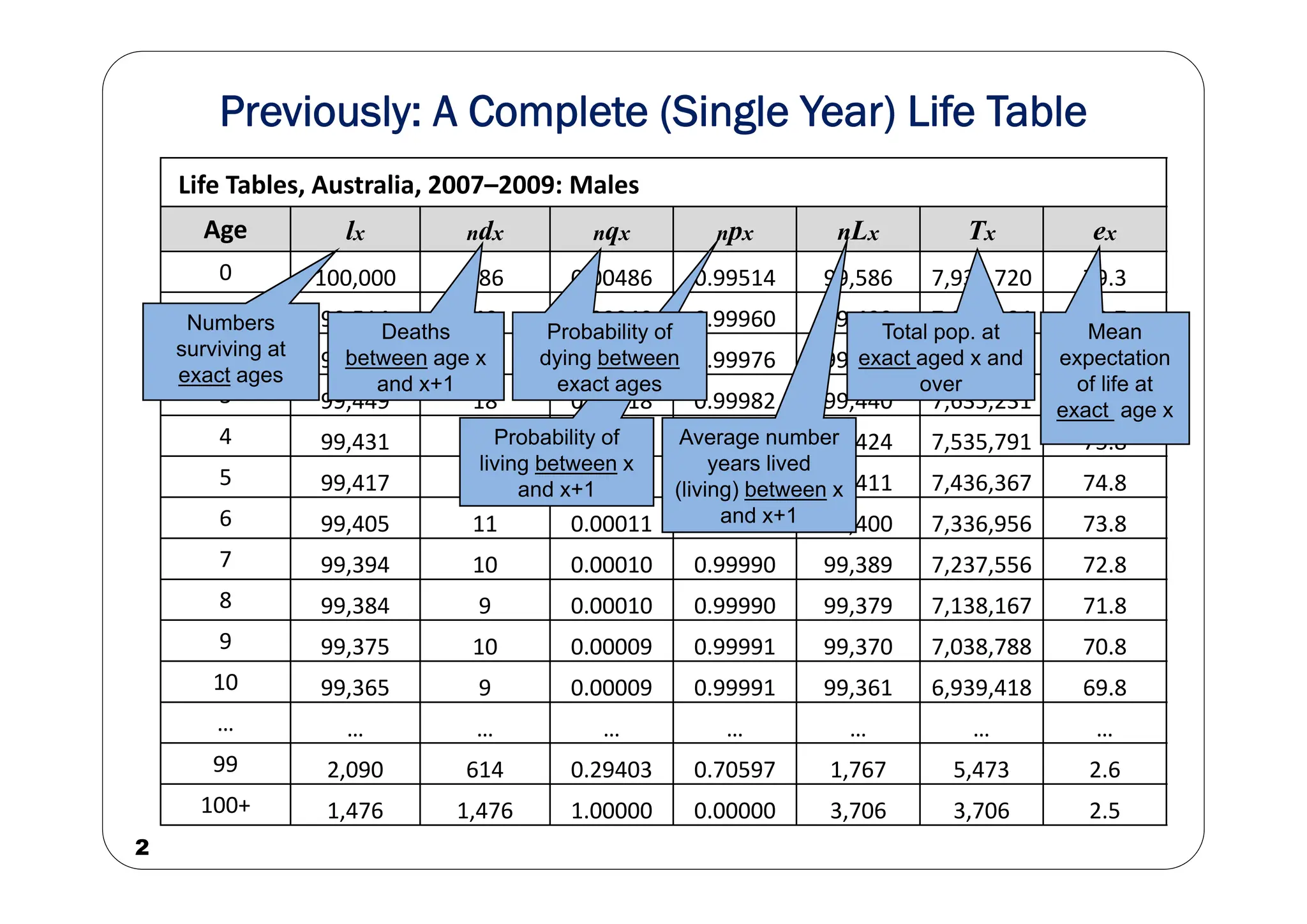
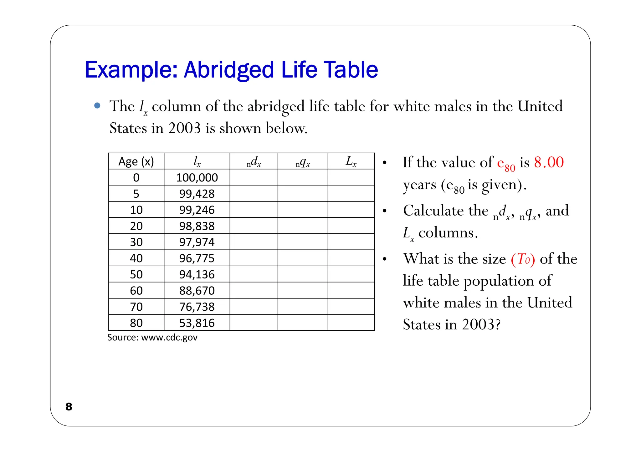
x lx ndx nqx Lx
0 100,000 572 0.00572 498,570
5 99,428 182 0.00183 496,685
10 99,246 408 0.00411 990,420
20 98,838 864 0.00874 984,060
30 97,974 1,199 0.01224 973,745
40 96,775 2,639 0.02727 954,555
50 94,136 5,466 0.05806 914,030
60 88,670 11,932 0.13457 827,040
70 76,738 22,922 0.29870 652,770
80 53,816 53,816 1.00000 430,528
T0 = 7,722,403
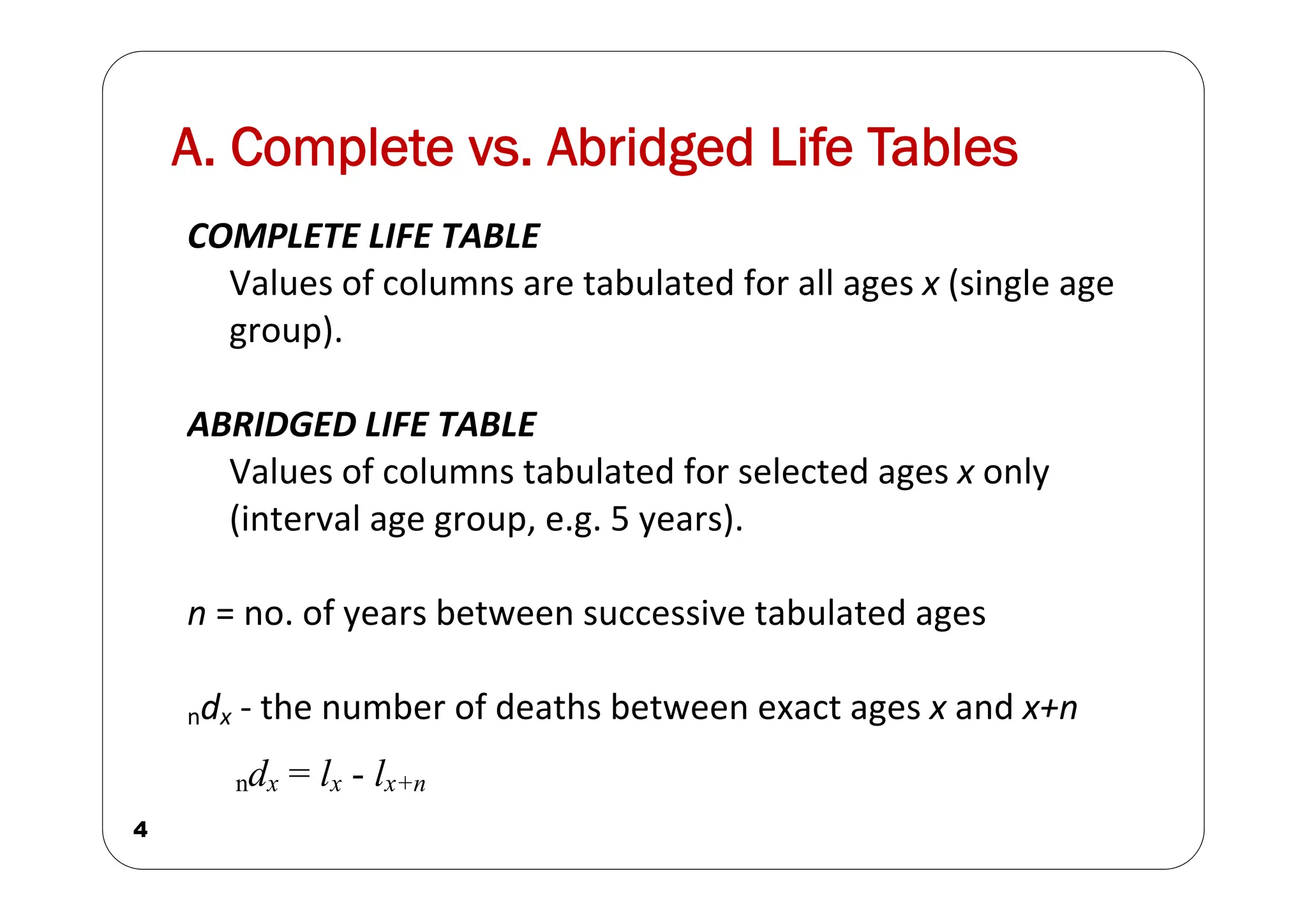
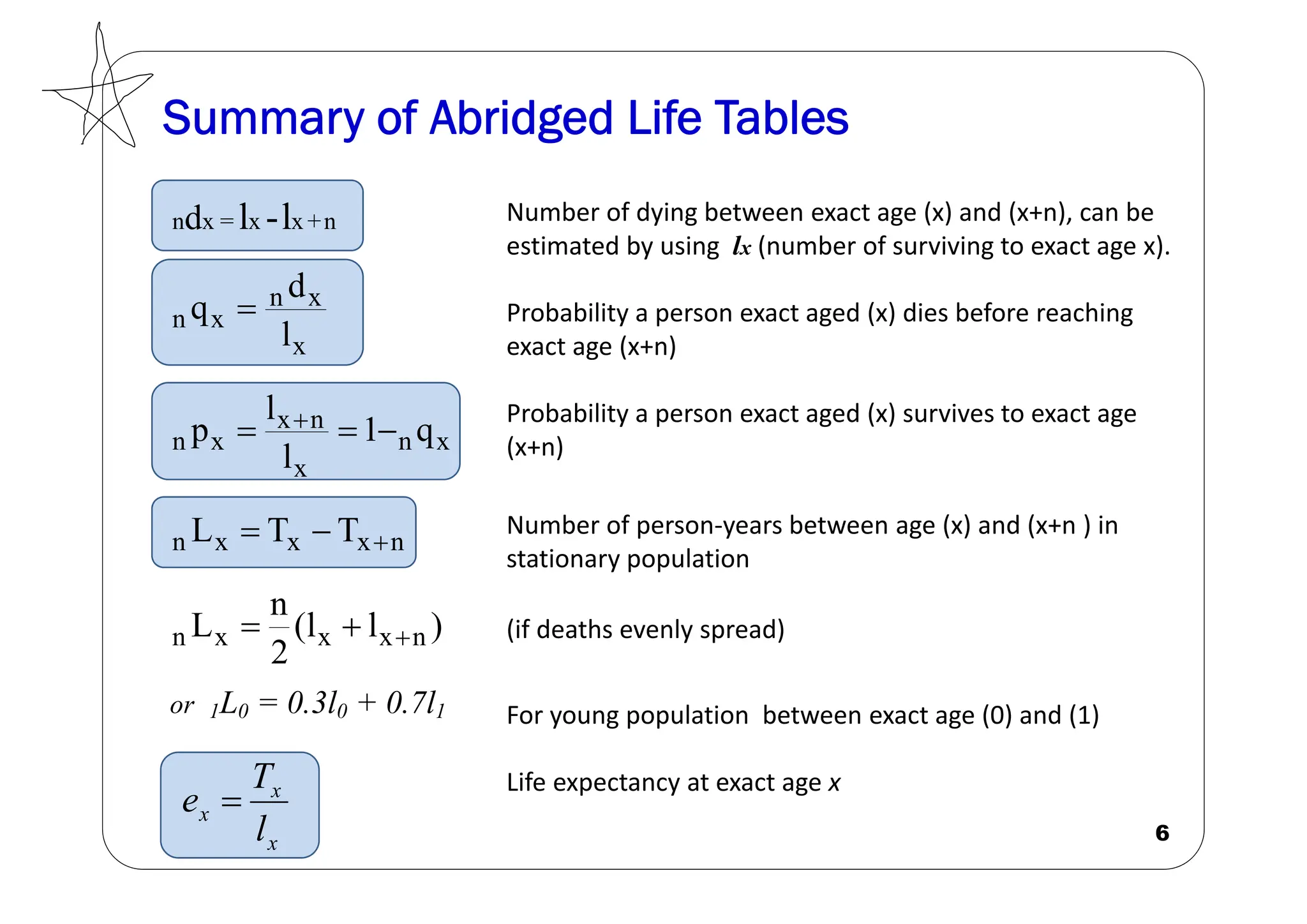
d(x) = l(x) – l(x+n)
d(0) = l(0) – l(5)
= 100,000 – 99,428
= 572
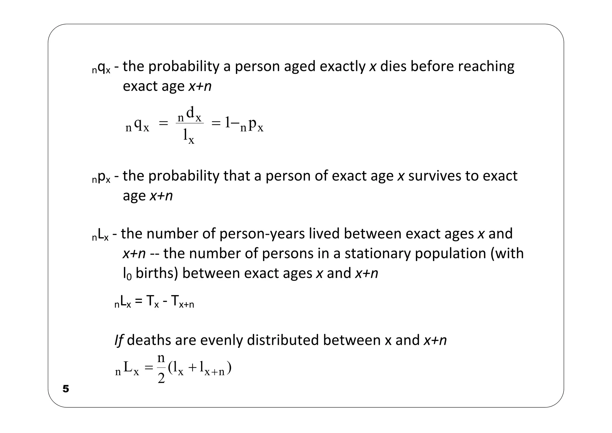
q(x) = d(x)/l(x)
q(0) = d(0)/l(x)
= 572/100,000
= 0.00572
Note: 5 decimal place
L(x) = n/2 . (l(x)+l(x+n),
or
L(x) = T(x)‐T(x+n)
L(0) = (5/2) [ l(0)+l(5) ]
= 2.5 (100000+99428)
= 498,570
T(x) = L(x)+L(x+n)+ ... L(n)
T(0) = L(0)+L(5)+ .... L(80)
= 498,570+496,685+ ....+430,528
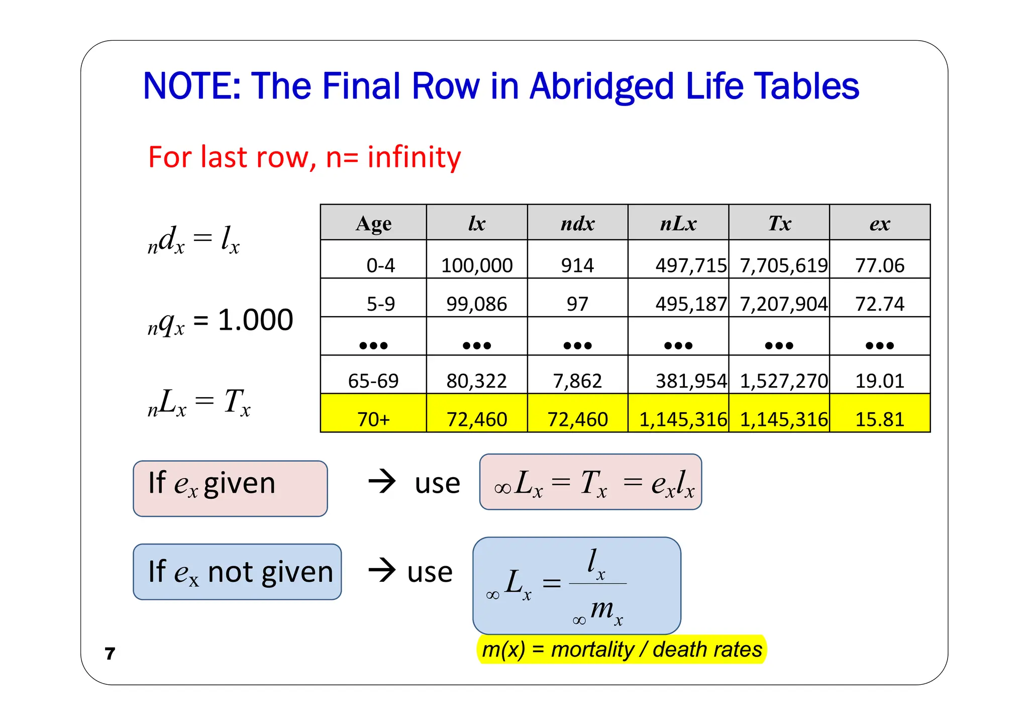
Last age group 80+
e(80) is given, thus:
L(80)= e(80) l(80)
= 8.0 x 53,816
= 430,528
n
5
5
10
10
10
10
10
10
10
∞

10. Complete Life Tables Abridged Life Tables
10
1
1 - 
 x
x
x l
l
d
x
x
x
l
d
q 1
1 
x
x
x
x q
l
l
p 1
1
1 1

 
1
1 

 x
x
x T
T
L
)
(
2
1
1
1 

 x
x
x l
l
L
or 1L0 = 0.3l0 + 0.7l1
x
x
x
l
T
e 
n
x
x
x
n l
l
d 
 -
x
x
n
x
n
l
d
q 
x
n
x
n
x
x
n q
l
l
p 

 
1
n
x
x
x
n T
T
L 


)
(
2
n
x
x
x
n l
l
n
L 


or 1L0 = 0.3l0 + 0.7l1
x
x
x
l
T
e 
n=1 n=interval
Last row L(x):
If e(x) is given, or
not given..

11. B. Life Table with Death Rates (ASDR = mx)
Observed Data for Age Specific Death Rates (ASDR) USA 1995
11
Deaths
Mid‐year
Population
ASDRs (Mx)
Age = (Death/Pop) x 1000
0‐4 35,976 19,591,148 (35,976/19,591,148) x1000= 1.836
5‐9 3,780 19,219,956 0.197
10‐14 4,816 18,914,532 0.255
15‐19 15,089 18,064,517 (15,089/18,064,517) x 1000= 0.835
20‐24 19,155 17,882,118 1.071
25‐29 22,681 19,005,343 1.193
30‐34 35,064 21,867,796 (35,064/ 21,867,796) x 1000= 1.603
35‐39 46,487 22,248,914 2.089
40‐44 55,783 20,218,805 2.759
45‐49 65,623 17,448,898 (65,623 /17,448,898) x1000 = 3.761
50‐54 77,377 13,629,862 5.677
55‐59 96,641 11,084,606 8.718
60‐64 138,871 10,046,478 (138,871/ 10,046,478)x1000= 13.823
65‐69 204,347 9,927,958 20.583
70+ 1,489,979 23,550,897 63.266
Total 2,311,669 262,701,828
Source: Rowland (2003)

12. B. Life Table with Death Rates (ASDR = mx)
12
Step 1: A set of ASDRx is needed.
Using these to compute nqx values:
)
2
n
(
1
n
)
(n
2
2n
x
n
x
n
x
n
x
n
x
n
m
m
m
m
q








(Note: mx isn’t per 1,000)
Step 2: Set l0 (say, 100,000)
Step 3. nq0 =
0
0
n
l
d
then compute nd0 = l0  nq0
Step 4: nd0 = l0 – ln so compute ln
Then compute the rest of columns in the life table.

13. 13
Assume deaths at age x are evenly spread over the interval x to x+1.
Therefore, the number of deaths between ages x and x+1/2
= 1dx / 2
No. of survivors to age x+1/2 = lx - 1dx /2
1mx =
2
d
l
d
x
1
x
x
1

=
2
q
1
q
x
1
x
1

where 1qx = (1dx / lx)
If nmx represents the ASDR per person for ages between x and x+n
exactly:
nqx =
x
n
x
n
m
m
n
2
2n



Relationship between ASDRx and 1qx

14. Computing A Life Table – with ASDR (mx)
14
n Age mx nqx lx ndx nLx Tx ex
5 0‐4 0.00184 0.00914 100,000 914 497,715 7,705,619 77.06
5 5‐9 0.00020 0.00098 99,086 97 495,187 7,207,904 72.74
5 10‐14 0.00025 0.00127 98,989 126 494,628 6,712,717 67.81
5 15‐19 0.00084 0.00417 98,863 412 493,283 6,218,089 62.90
5 20‐24 0.00107 0.00534 98,451 526 490,939 5,724,806 58.15
5 25‐29 0.00119 0.00595 97,925 583 488,167 5,233,867 53.45
5 30‐34 0.00160 0.00799 97,342 777 484,768 4,745,700 48.75
5 35‐39 0.00209 0.01039 96,565 1,004 480,316 4,260,932 44.13
5 40‐44 0.00276 0.01370 95,561 1,309 474,534 3,780,616 39.56
5 45‐49 0.00376 0.01863 94,252 1,756 466,871 3,306,083 35.08
5 50‐54 0.00568 0.02799 92,496 2,589 456,009 2,839,212 30.70
5 55‐59 0.00872 0.04266 89,907 3,836 439,948 2,383,202 26.51
5 60‐64 0.01382 0.06681 86,072 5,750 415,984 1,943,254 22.58
5 65‐69 0.02058 0.09788 80,322 7,862 381,954 1,527,270 19.01
∞ 70+ 0.06327 1.00000 72,460 72,460 1,145,316 1,145,316 15.81
)
m
(n
2
m
2n
x
n
x
n




x
n q (Note: n = 5 years, and mx is not per 1,000)

15. 15
n Age mx nqx lx ndx nLx Tx ex
5 0‐4 0.00184 0.00914 100,000 914 497,715 7,705,619 77.06
5 5‐9 0.00020 0.00098 99,086 97 495,187 7,207,904 72.74
5 10‐14 0.00025 0.00127 98,989 126 494,628 6,712,717 67.81
5 15‐19 0.00084 0.00417 98,863 412 493,283 6,218,089 62.90
… … … … … … … … …
5 65‐69 0.02058 0.09788 80,322 7,862 381,954 1,527,270 19.01
∞ 70+ 0.06327 1.00000 72,460 72,460 1,145,316 1,145,316 15.81
n Age lx nqx ndx nLx Tx ex
5 0‐4 100,000 0.00914 914 497,715 7,705,619 77.06
5 5‐9 99,086 0.00098 97 495,187 7,207,904 72.74
5 10‐14 98,989 0.00127 126 494,628 6,712,717 67.81
5 15‐19 98,863 0.00417 412 493,283 6,218,089 62.90
… … … … … … … …
5 65‐69 80,322 0.09788 7,862 381,954 1,527,270 19.01
∞ 70+ 72,460 1.00000 72,460 1,145,316 1,145,316 15.81
ComputingA LifeTable withoutASDR (mx)
ComputingA LifeTable withASDR (mx) – Roland’s Chapter 8

16. C. Stationary Population
16
‐ It is defined as a population whose total size and age
distribution remain constant over time.
If a population
a) is closed to migration
b) has number of births = number of deaths
c) has constant mortality in accordance with a fixed set
of ASDRs
Then, it will be stationary.

17. 17
nLx column of a life table represents a
stationary population with l0 births per year
nLx represents the number aged x to x+n‐1 last
birthday and is the age distribution of the
population.

18. Crude Birth Rate (CBR) & Crude Death Rate (CDR)
for a Stationary Population
18
Annual no. of births = l0
Annual no. of deaths = l0
Total population size = T0
0
0
0 000
1
000
1
e
T
l
CDR
CBR
,
, 




19. D. Period vs. Cohort Life Table
19
 Period life table
It uses the probability of death of people from different
ages in a particular year (i.e. current year).
 Cohort LifeTable
It used the probability of death of people from a given cohort
(especially birth year) over the course of their lifetime.
"Life table" primarily refers to period life tables, as cohort life
tables can only be constructed using data up to the current point,
and distant projections for future mortality.

20. Uses of Life Tables (Next Week)
20
(1) Measuring population mortality
The most commonly used
(2) Evaluation of mortality risk factors & effectiveness
Used by epidemiologist/health professionals
(3) Life assurance and superannuation valuations

21. 21
Life tables are used to represent the survivorship of a past
generation but are more usually used to represent the
survivorship of a future cohort if that cohort experiences
theASDRs of a specified time period.
 Life tables are used
 to represent survivorship from age to age
 to measure life expectancy
 in measuring reproductivity
 in population projections.