Downloaded 39 times


![Financial mathematics
Actuarial mathematics calculation applies probability to
quantify uncertainty on present values calculation.
capitals <- c(-1000,200,500,700)
times <- c(0,1,2,5)
#calculate a present value
presentValue(cashFlows=capitals, timeIds=times,
interestRates=0.03)
## [1] 269.2989](https://image.slidesharecdn.com/introtolifecontingencies-150427022644-conversion-gate01/85/Introduction-to-lifecontingencies-R-package-12-320.jpg)
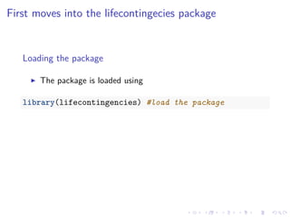
![Financial mathematics
Actuarial mathematics calculation applies probability to
quantify uncertainty on present values calculation.
Certain present value calculations can be directly evaluated by
the package
capitals <- c(-1000,200,500,700)
times <- c(0,1,2,5)
#calculate a present value
presentValue(cashFlows=capitals, timeIds=times,
interestRates=0.03)
## [1] 269.2989](https://image.slidesharecdn.com/introtolifecontingencies-150427022644-conversion-gate01/85/Introduction-to-lifecontingencies-R-package-13-320.jpg)
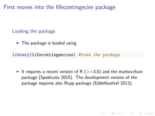
![The presentValue function is the kernel of functions that are
used to calculate annuities and accumulated values, also paid
in fractional k payments.
ann1 <- annuity(i=0.03, n=5, k=1, type="immediate")
ann2 <- annuity(i=0.03, n=5, k=12, type="due")
c(ann1,ann2)
## [1] 4.579707 4.653791](https://image.slidesharecdn.com/introtolifecontingencies-150427022644-conversion-gate01/85/Introduction-to-lifecontingencies-R-package-14-320.jpg)
![Such functions can be combined to price bonds and other
classical financial products.
bondPrice<-5*annuity(i=0.03,n=10)+100*1.03^-10
bondPrice
## [1] 117.0604](https://image.slidesharecdn.com/introtolifecontingencies-150427022644-conversion-gate01/85/Introduction-to-lifecontingencies-R-package-15-320.jpg)
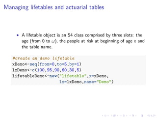
![Such functions can be combined to price bonds and other
classical financial products.
The following code exemplifies the calculation of a 5% coupon
bond at 3% yield rate when the term is ten year.
bondPrice<-5*annuity(i=0.03,n=10)+100*1.03^-10
bondPrice
## [1] 117.0604](https://image.slidesharecdn.com/introtolifecontingencies-150427022644-conversion-gate01/85/Introduction-to-lifecontingencies-R-package-16-320.jpg)
![In practice, it is often more convenient to load an existing table
from a CSV or XLS source. Some common tables have been
bundled as data.frames within the package.
data(demoIta) #using the internal Italian LT data set
lxIPS55M <- with(demoIta, IPS55M)
#performing some fixings
pos2Remove <- which(lxIPS55M %in% c(0,NA))
lxIPS55M <-lxIPS55M[-pos2Remove]
xIPS55M <-seq(0,length(lxIPS55M)-1,1)
#creating the table
ips55M <- new("lifetable",x=xIPS55M,
lx=lxIPS55M,name="IPS 55 Males")](https://image.slidesharecdn.com/introtolifecontingencies-150427022644-conversion-gate01/85/Introduction-to-lifecontingencies-R-package-18-320.jpg)
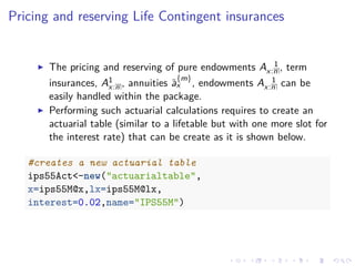
![In practice, it is often more convenient to load an existing table
from a CSV or XLS source. Some common tables have been
bundled as data.frames within the package.
The example that follows creates the Italian IPS55 life table.
data(demoIta) #using the internal Italian LT data set
lxIPS55M <- with(demoIta, IPS55M)
#performing some fixings
pos2Remove <- which(lxIPS55M %in% c(0,NA))
lxIPS55M <-lxIPS55M[-pos2Remove]
xIPS55M <-seq(0,length(lxIPS55M)-1,1)
#creating the table
ips55M <- new("lifetable",x=xIPS55M,
lx=lxIPS55M,name="IPS 55 Males")](https://image.slidesharecdn.com/introtolifecontingencies-150427022644-conversion-gate01/85/Introduction-to-lifecontingencies-R-package-19-320.jpg)
![It is therefore easy to perform standard demographic
calculations with the aid of package functions.
# decrements between age 65 and 70
dxt(ips55M, x = 65, t = 5)
## [1] 3659.74
# probabilities of death between age 80 and 85
qxt(ips55M, x = 80, t = 2)
## [1] 0.07264833
# expected curtate lifetime
exn(ips55M, x = 65)
## [1] 21.96873](https://image.slidesharecdn.com/introtolifecontingencies-150427022644-conversion-gate01/85/Introduction-to-lifecontingencies-R-package-20-320.jpg)

![The example that follows computes the yearly premium
P = 50000 ∗ 35E30
¨a
30:35
for a pure endowment on 50K capital.
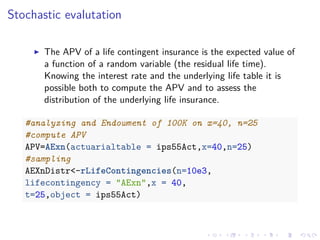
#compute APV
APV=50e3*Exn(actuarialtable =
ips55Act,x=30,n=35)
#compute Premium
P=APV/axn(actuarialtable =
ips55Act,x=30,n=35)
c(APV,P)
## [1] 23584.7564 938.1422](https://image.slidesharecdn.com/introtolifecontingencies-150427022644-conversion-gate01/85/Introduction-to-lifecontingencies-R-package-23-320.jpg)
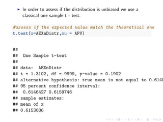

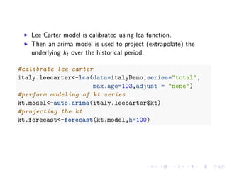
![-The code below generates the matrix of prospective life tables
#indexing the kt
kt.full<-ts(union(italy.leecarter$kt, kt.forecast$mean),
start=1872)
#getting and defining the life tables matrix
mortalityTable<-exp(italy.leecarter$ax
+italy.leecarter$bx%*%t(kt.full))
rownames(mortalityTable)<-seq(from=0, to=103)
colnames(mortalityTable)<-seq(from=1872,
to=1872+dim(mortalityTable)[2]-1)](https://image.slidesharecdn.com/introtolifecontingencies-150427022644-conversion-gate01/85/Introduction-to-lifecontingencies-R-package-34-320.jpg)
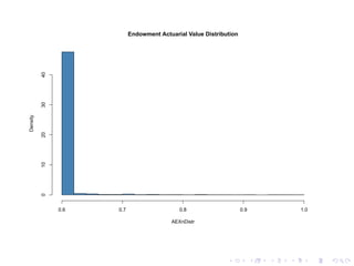
![now we need a function that returns the one-year death
probabilities given a year of birth (cohort.
getCohortQx<-function(yearOfBirth)
{
colIndex<-which(colnames(mortalityTable)
==yearOfBirth) #identify
#the column corresponding to the cohort
#definex the probabilities from which
#the projection is to be taken
maxLength<-min(nrow(mortalityTable)-1,
ncol(mortalityTable)-colIndex)
qxOut<-numeric(maxLength+1)
for(i in 0:maxLength)
qxOut[i+1]<-mortalityTable[i+1,colIndex+i]
#fix: we add a fictional omega age where
#death probability = 1
qxOut<-c(qxOut,1)
return(qxOut)
}](https://image.slidesharecdn.com/introtolifecontingencies-150427022644-conversion-gate01/85/Introduction-to-lifecontingencies-R-package-36-320.jpg)
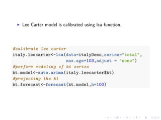
![Now we can evaluate ¨a65 and ˚e65 for workers born in 1920,
1950 and 1980 respectively.
cat("Results for 1920 cohort","n")
## Results for 1920 cohort
c(exn(at1920,x=65),axn(at1920,x=65))
## [1] 16.51391 15.14127
cat("Results for 1950 cohort","n")
## Results for 1950 cohort
c(exn(at1950,x=65),axn(at1950,x=65))
## [1] 18.72669 16.83391
cat("Results for 1980 cohort","n")](https://image.slidesharecdn.com/introtolifecontingencies-150427022644-conversion-gate01/85/Introduction-to-lifecontingencies-R-package-39-320.jpg)


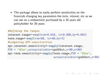
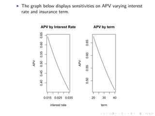
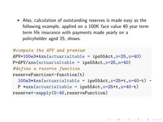
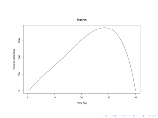
The document introduces the lifecontingencies R package, which merges demographic and financial mathematics functionalities for actuarial evaluations of life-contingent insurances. It outlines various functionalities such as loading the package, performing financial and demographic calculations, and assessing mortality impacts on annuities. Additionally, it showcases examples for pricing and reserving insurance products, managing life tables, and utilizing demographic models for projections.


![[Actuary] actuarial mathematics and life table statistics](https://cdn.slidesharecdn.com/ss_thumbnails/actuaryactuarialmathematicsandlife-tablestatistics-120627131254-phpapp01-thumbnail.jpg?width=640&height=640&fit=bounds)


![[P.D.F] Computational Actuarial Science with R For Kindle](https://cdn.slidesharecdn.com/ss_thumbnails/computational-actuarial-science-with-r-191110184553-thumbnail.jpg?width=640&height=640&fit=bounds)


