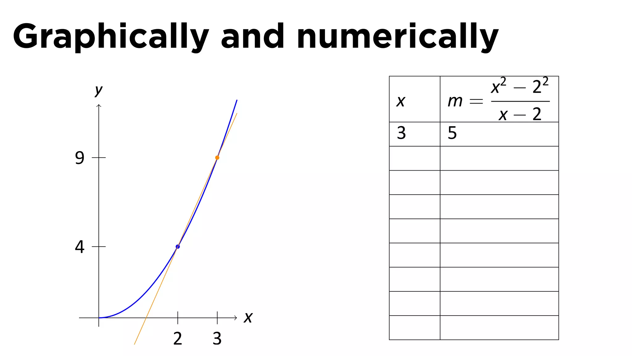
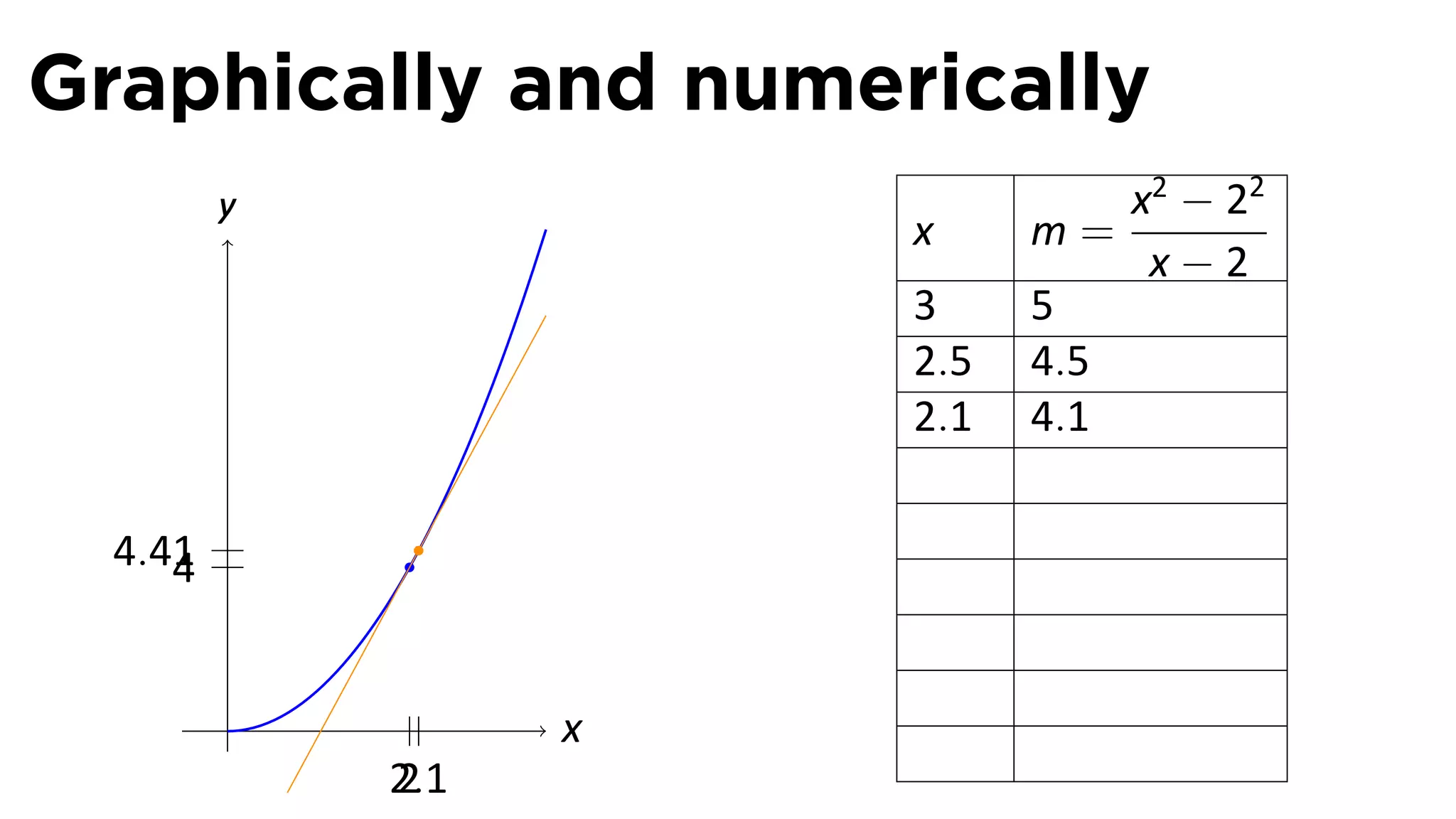
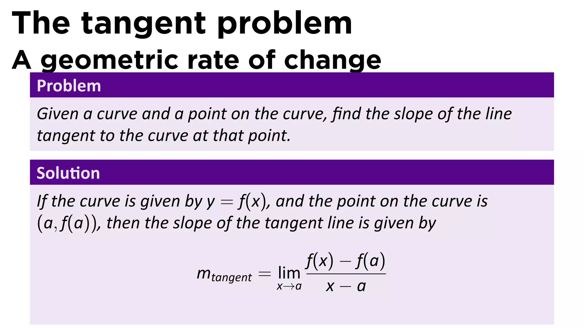
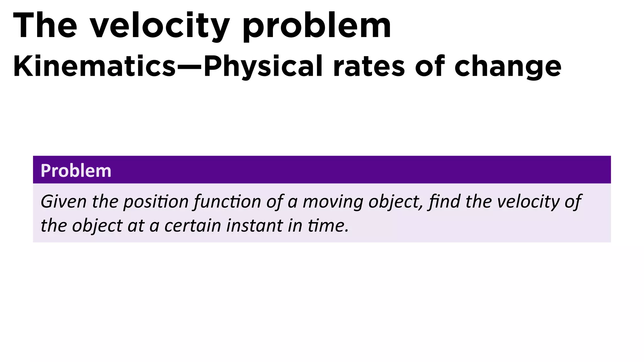
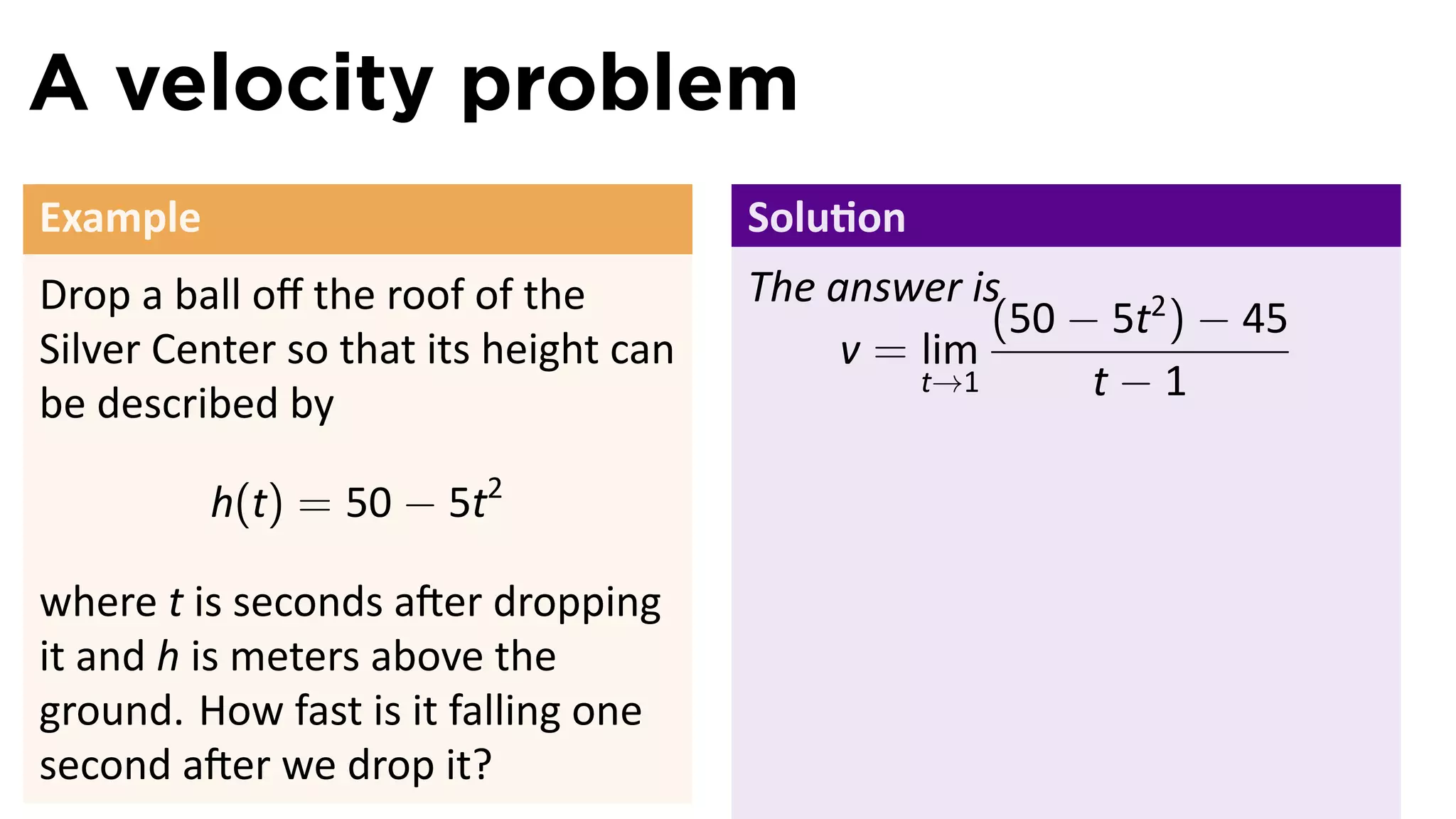
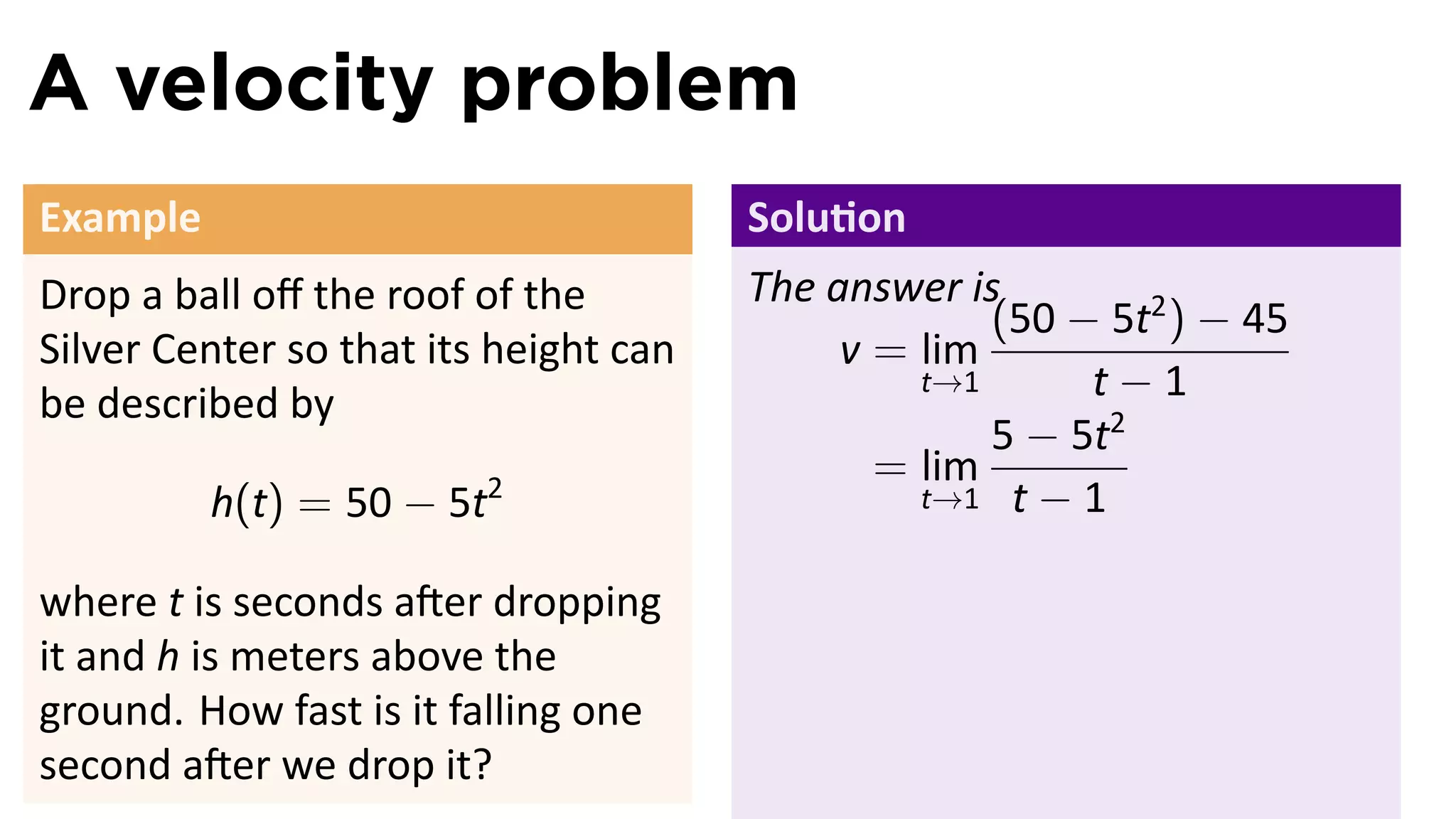
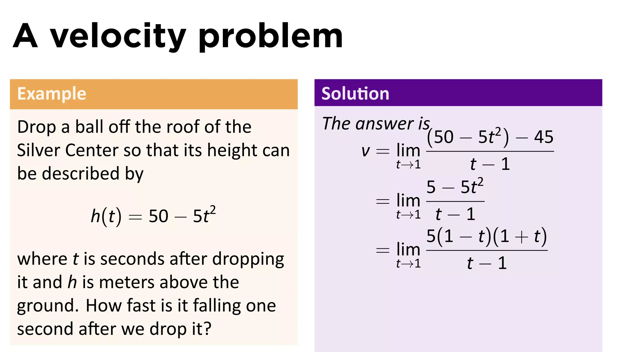
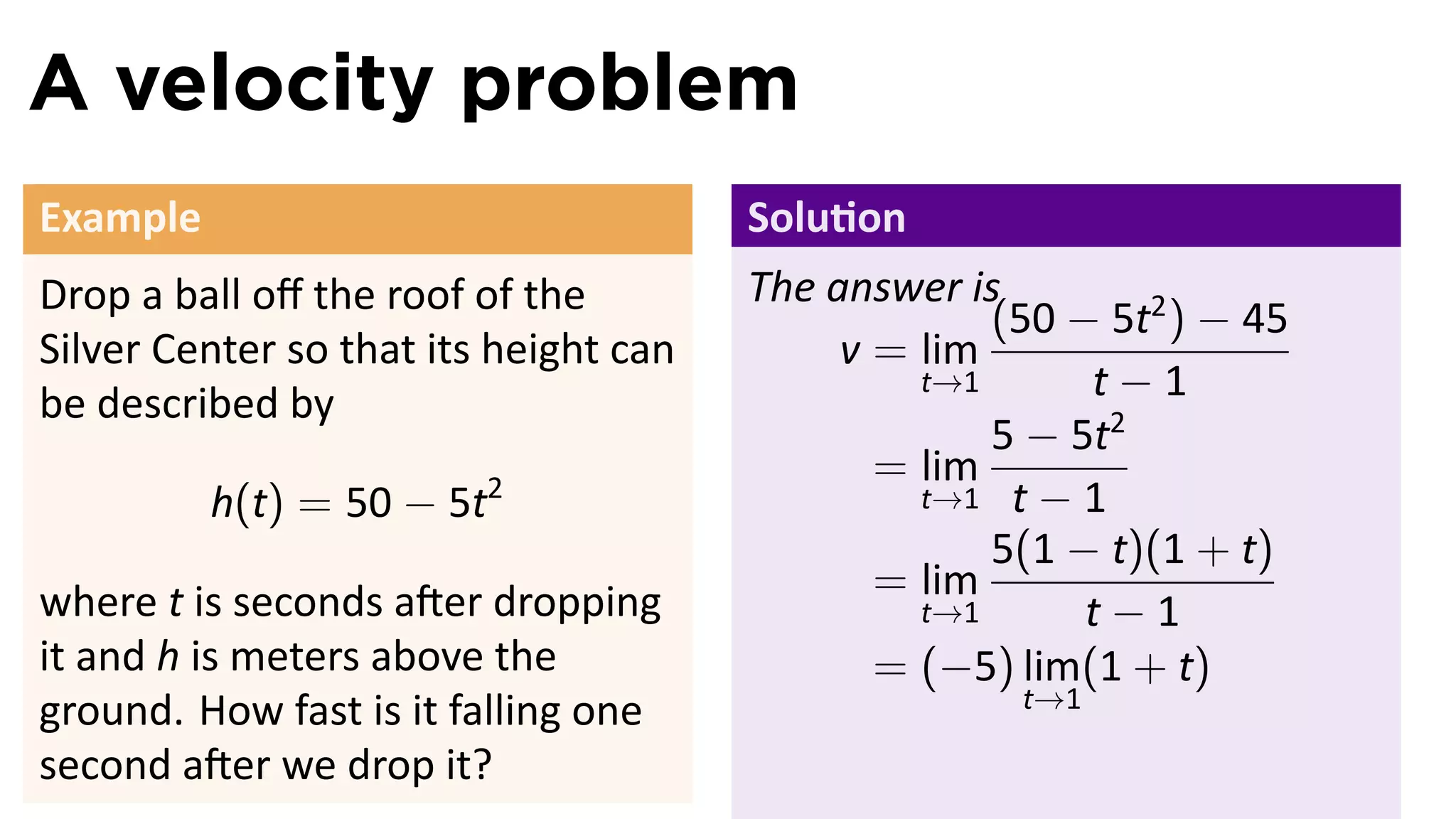
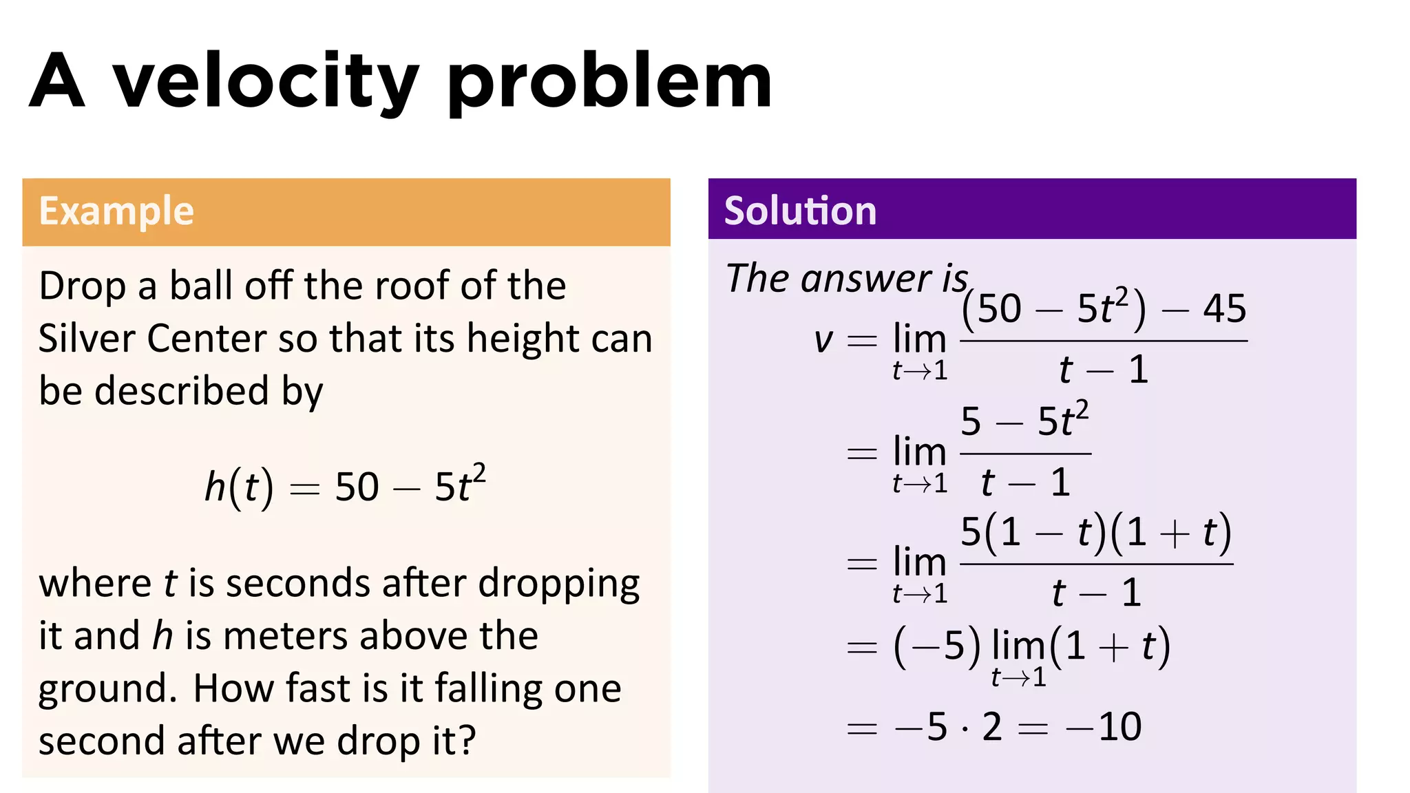
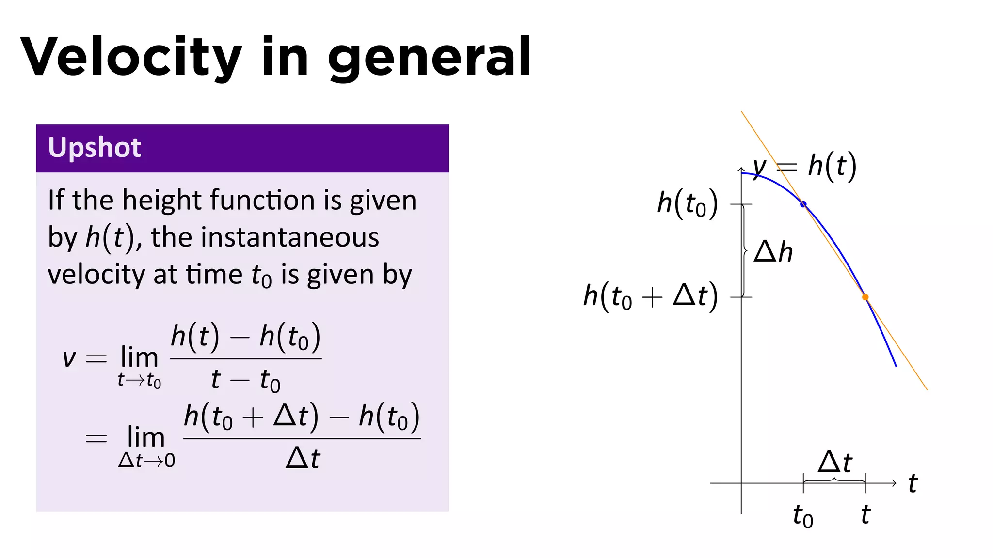
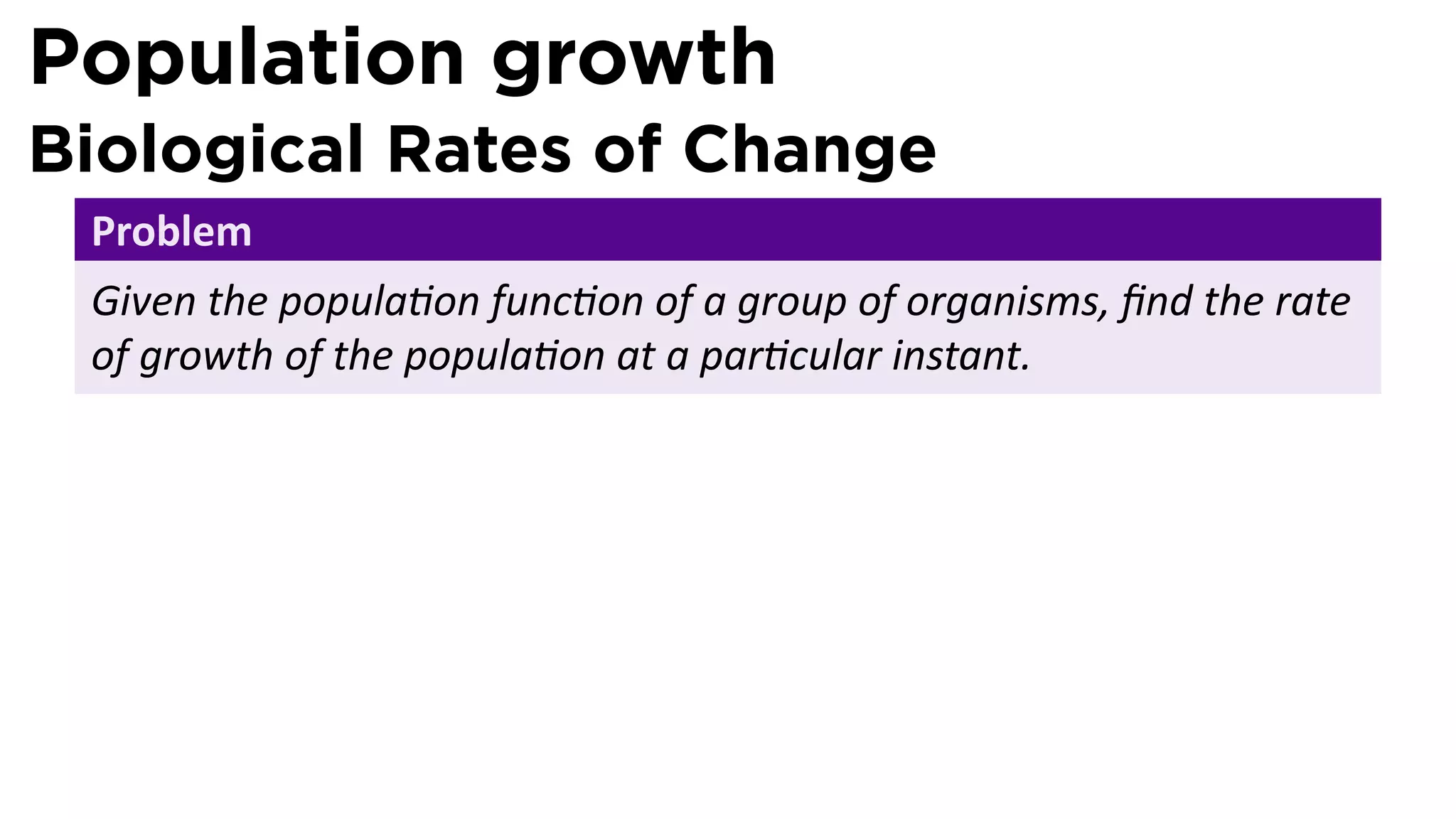
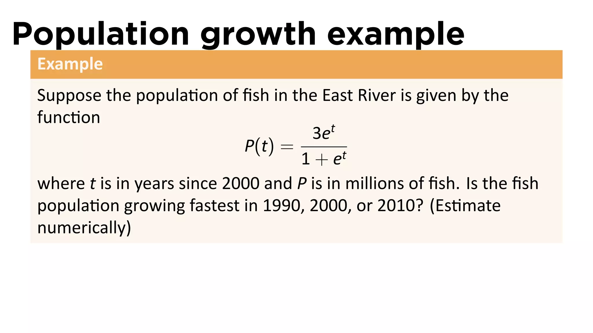
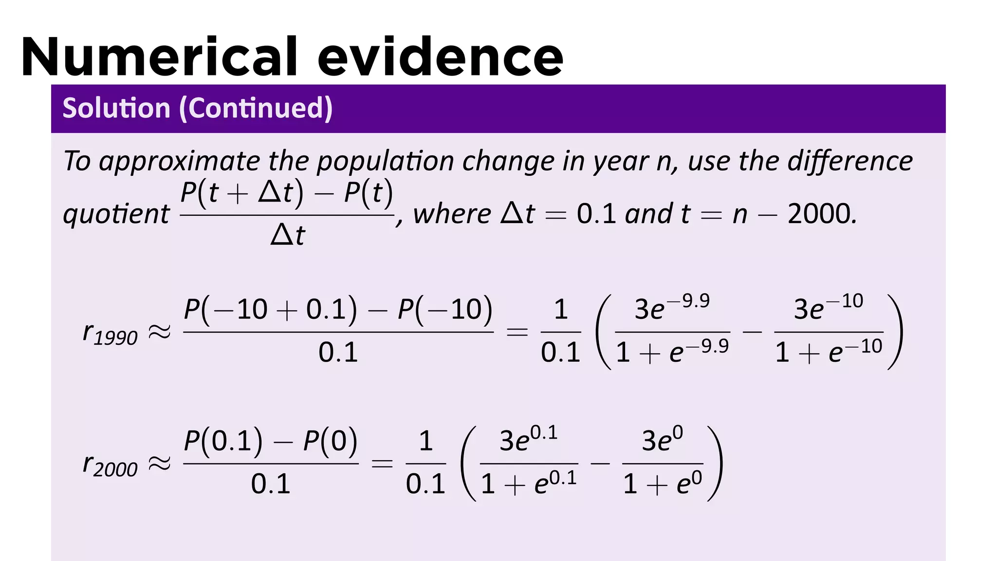
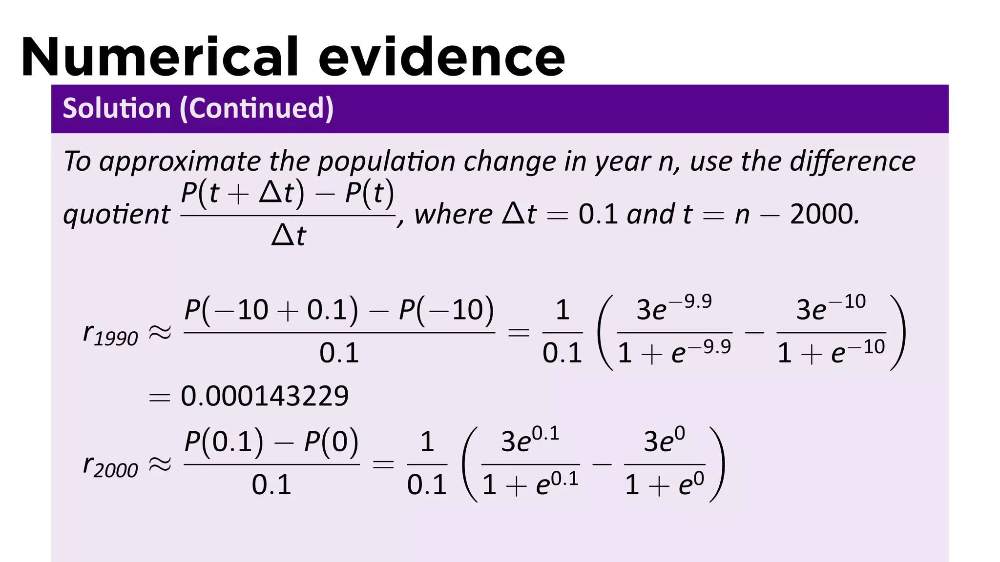
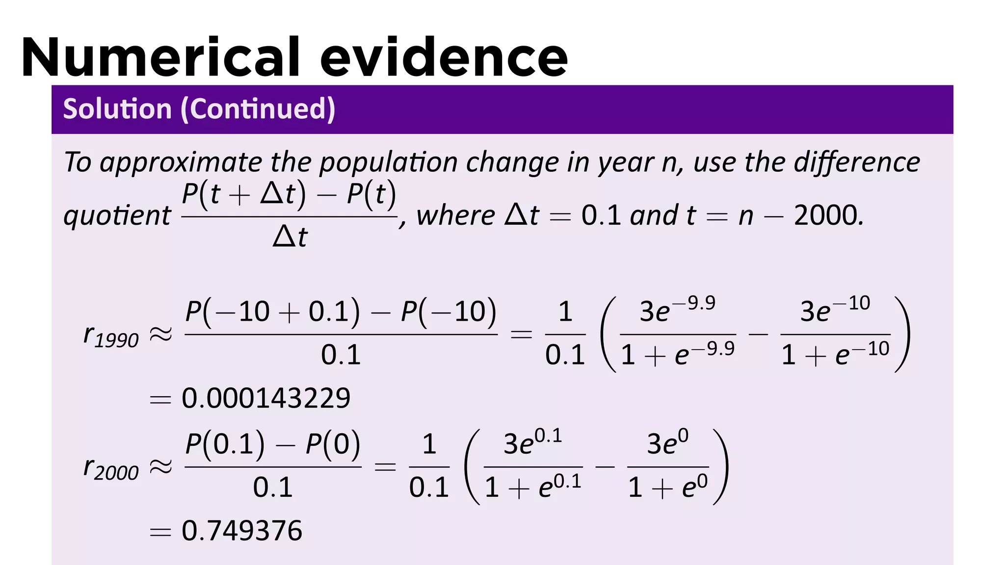
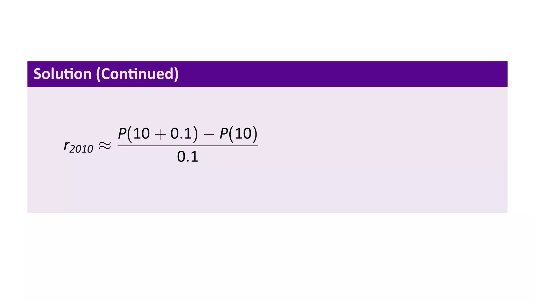
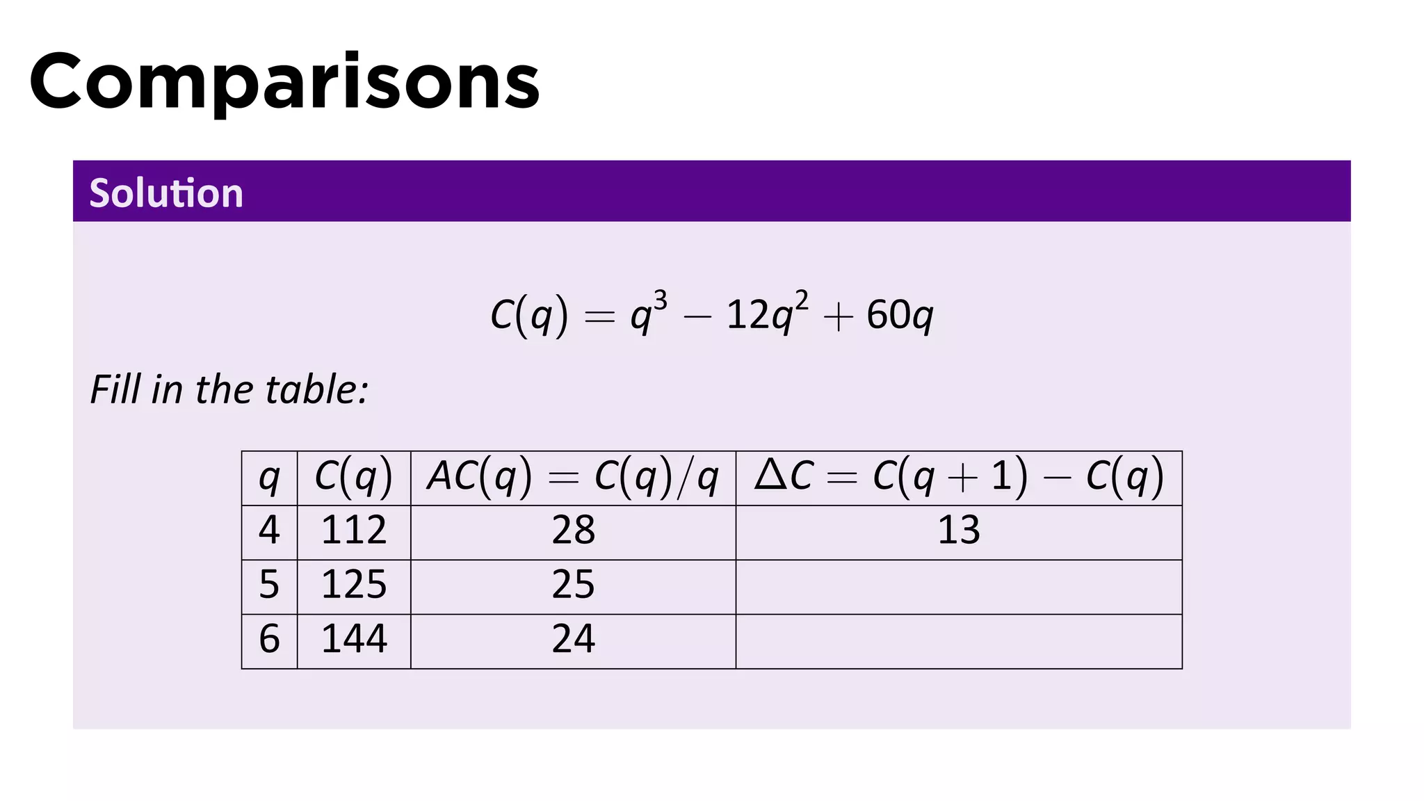
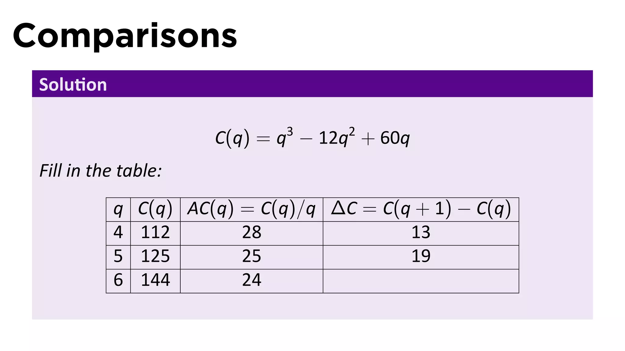
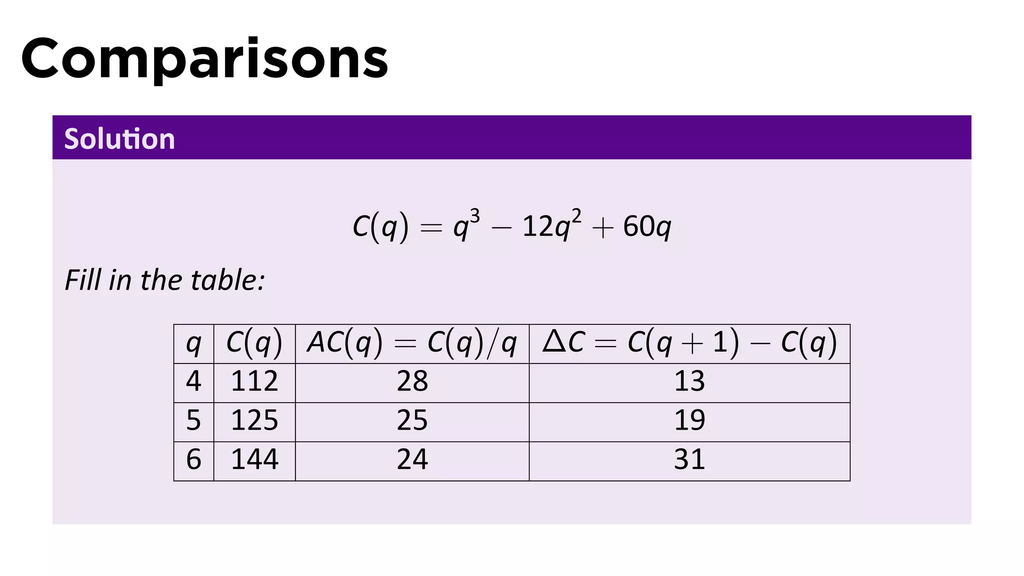
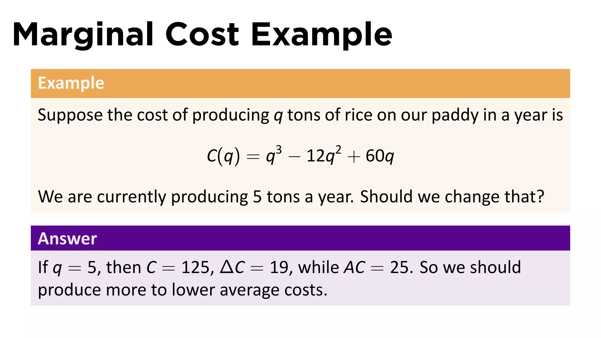
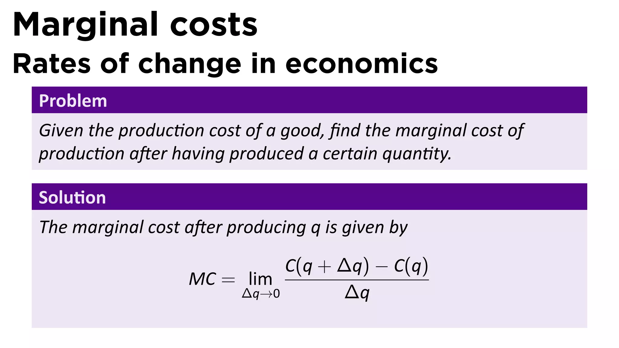
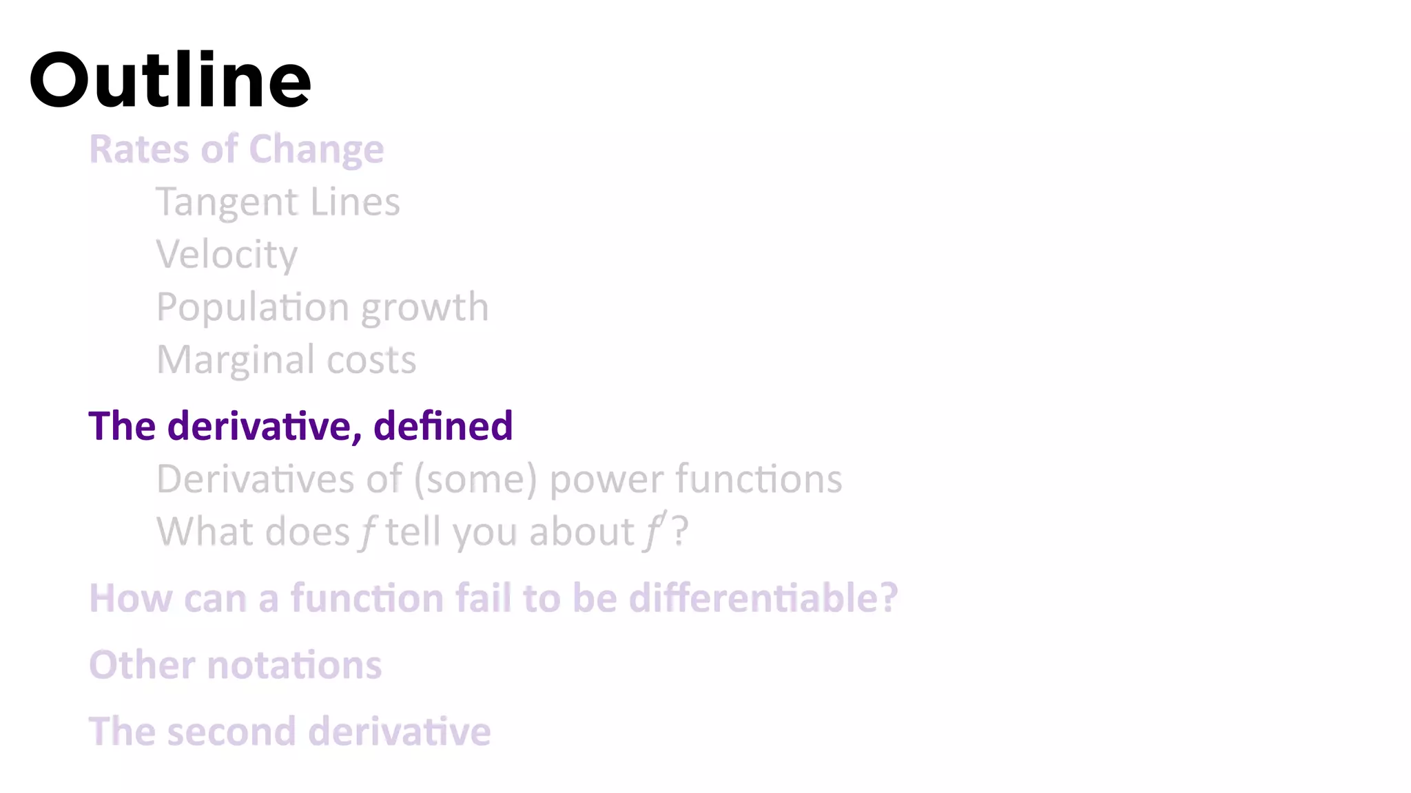
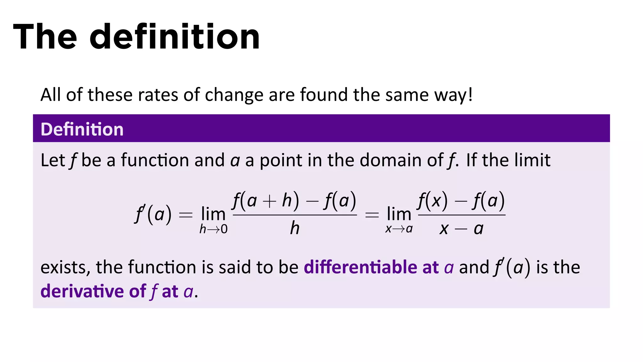
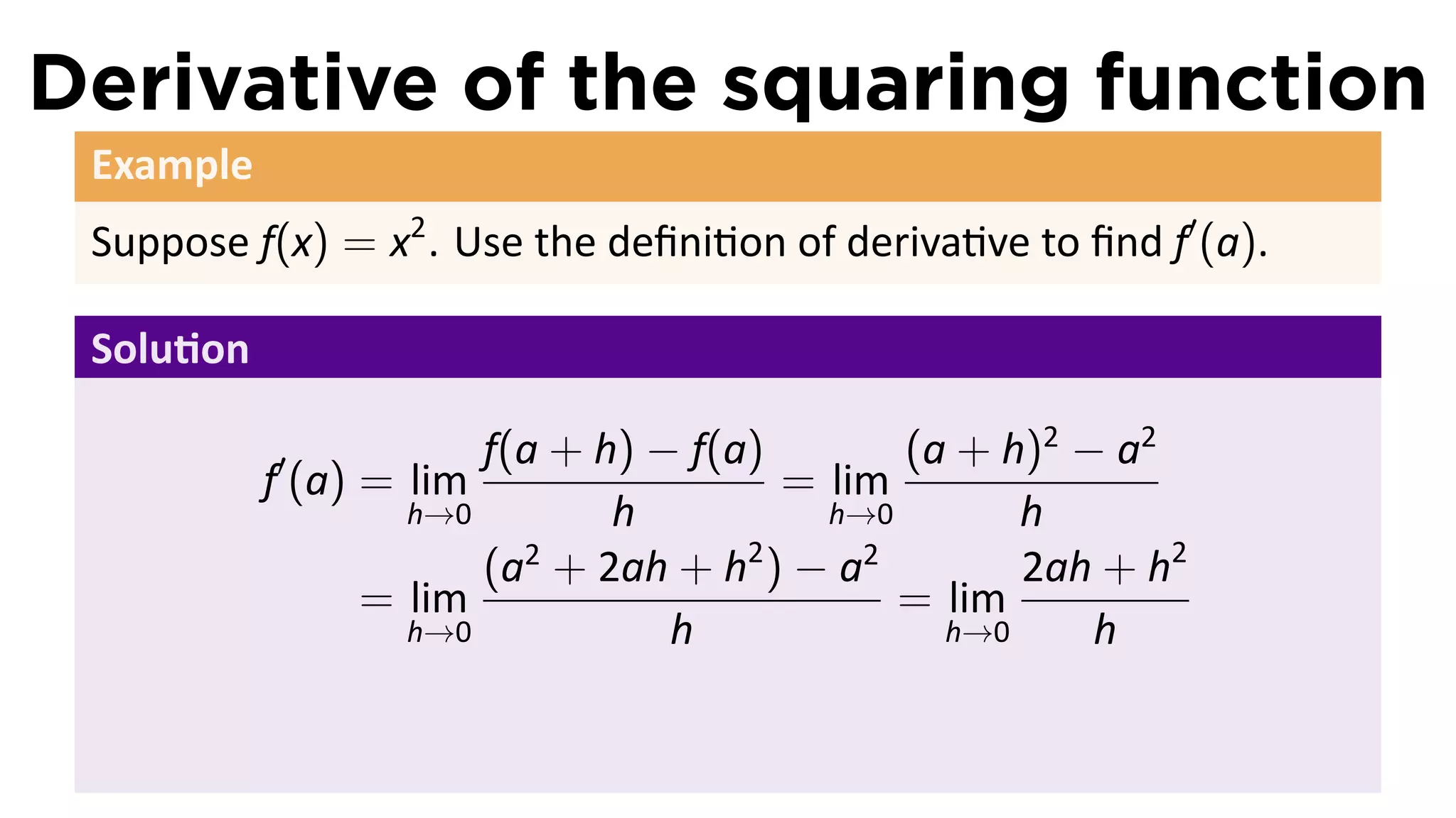
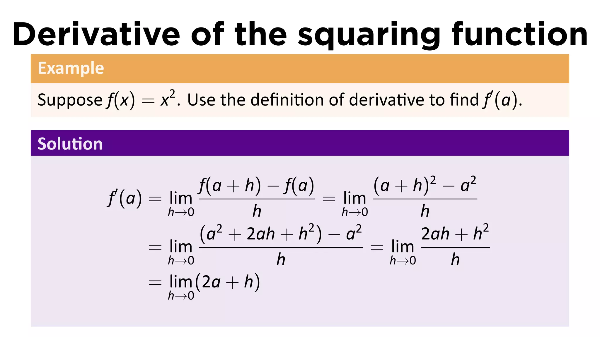
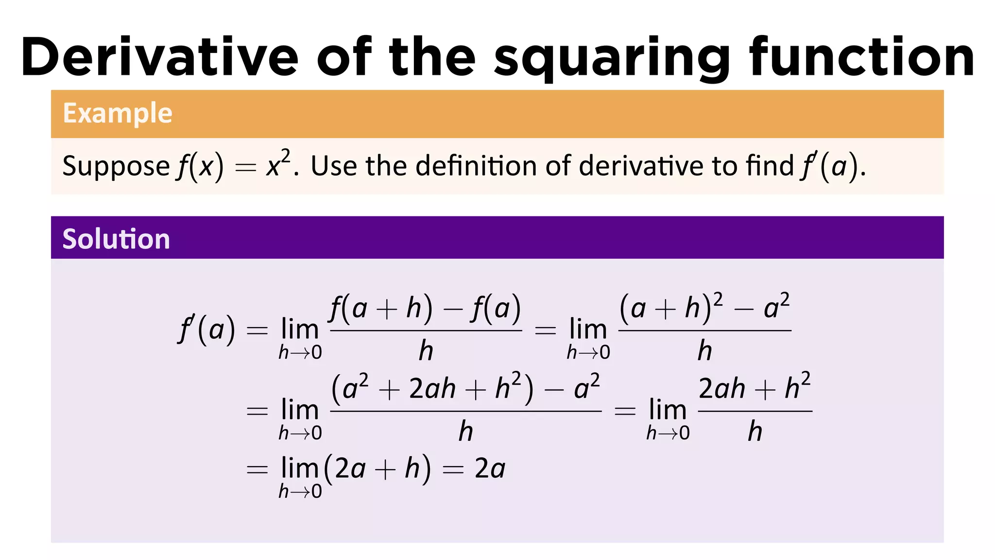
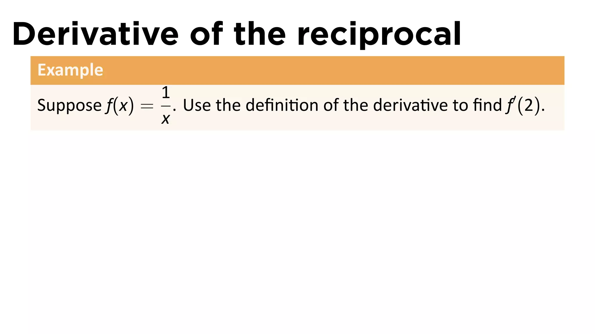
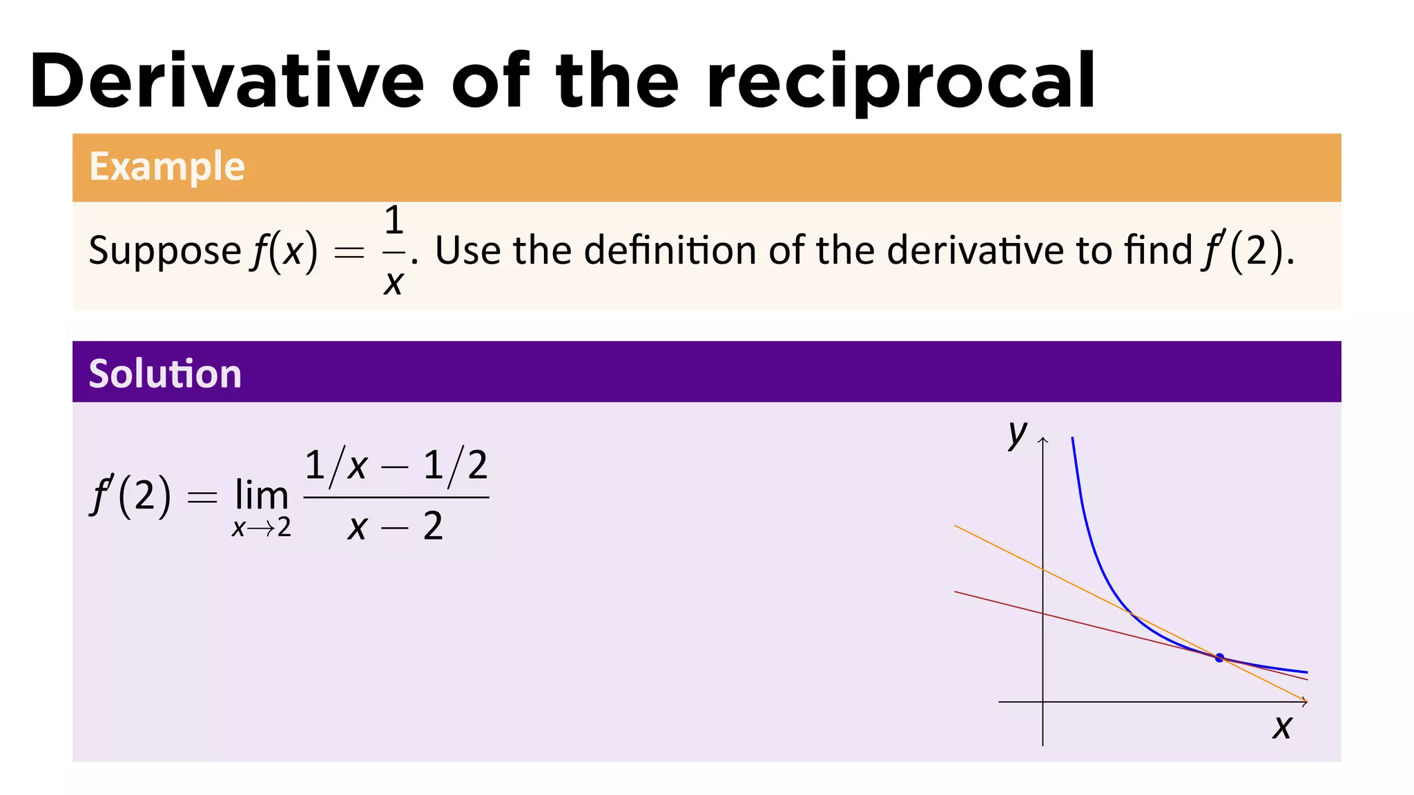
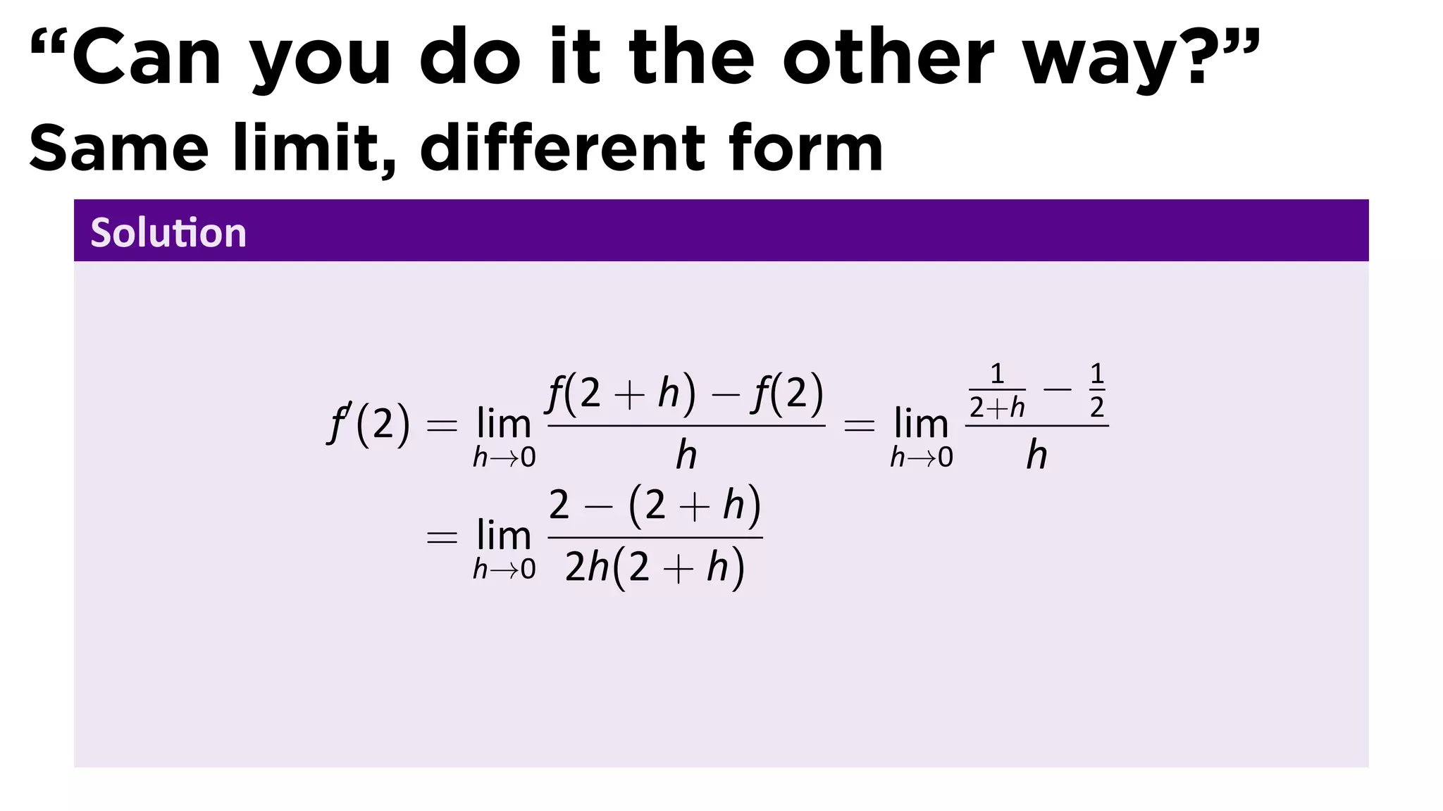
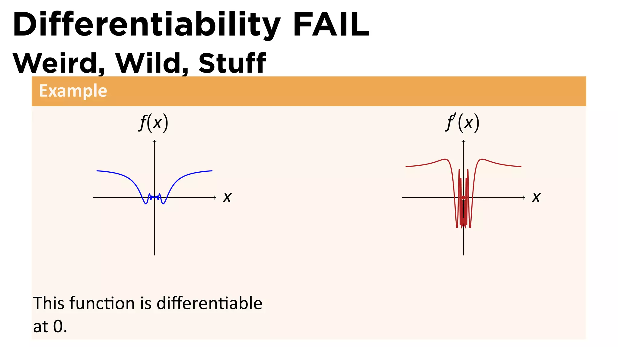
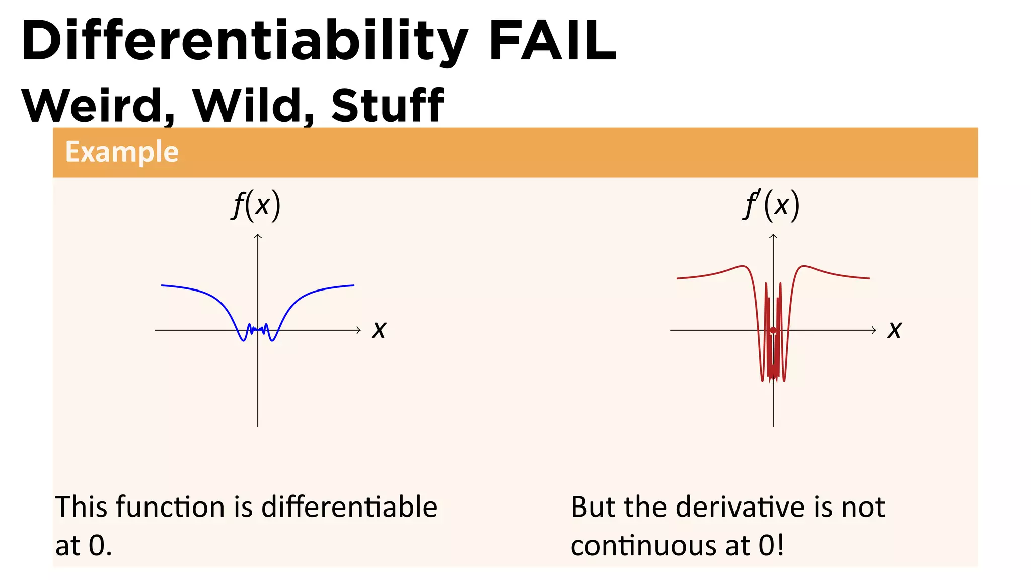
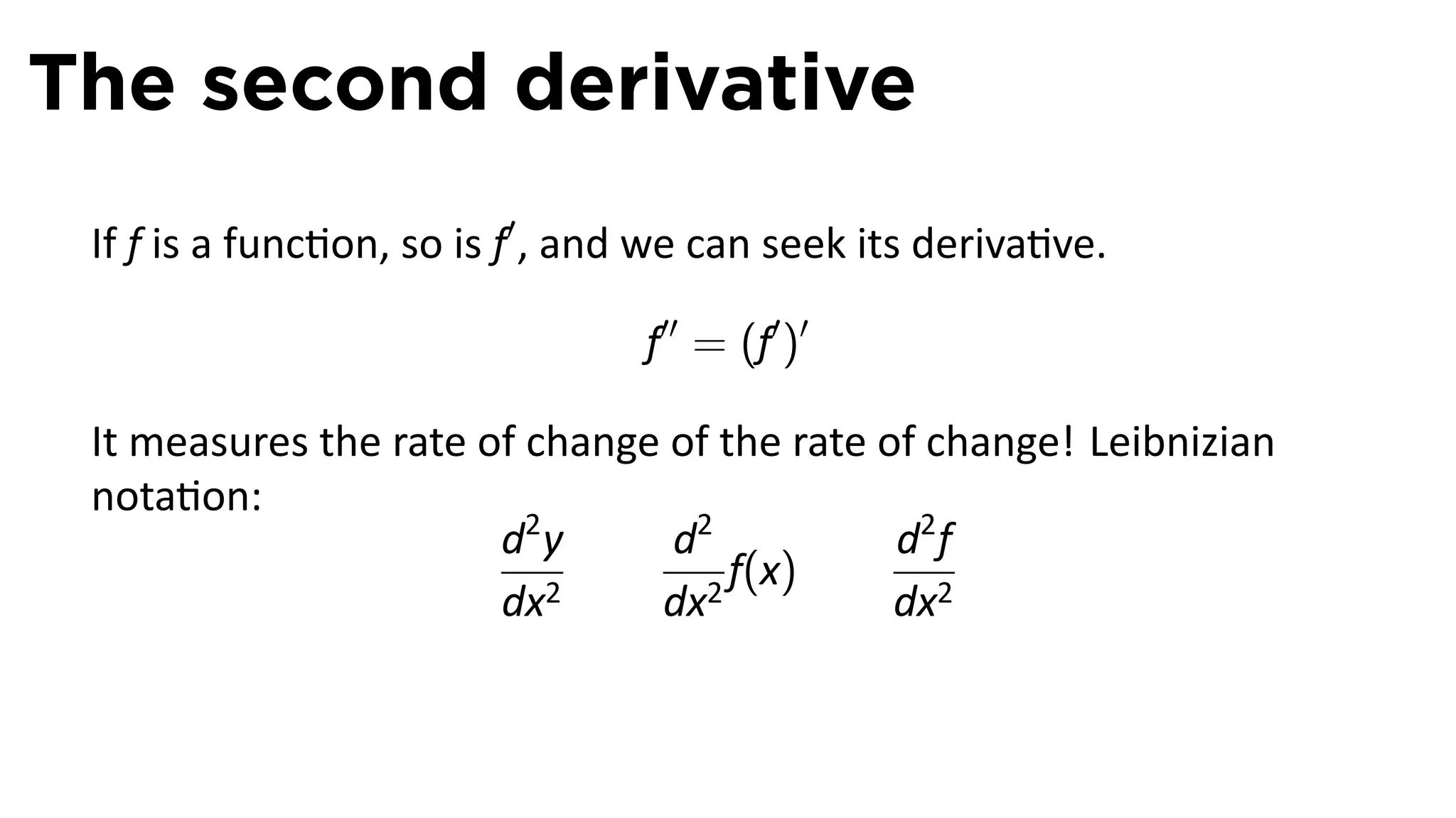
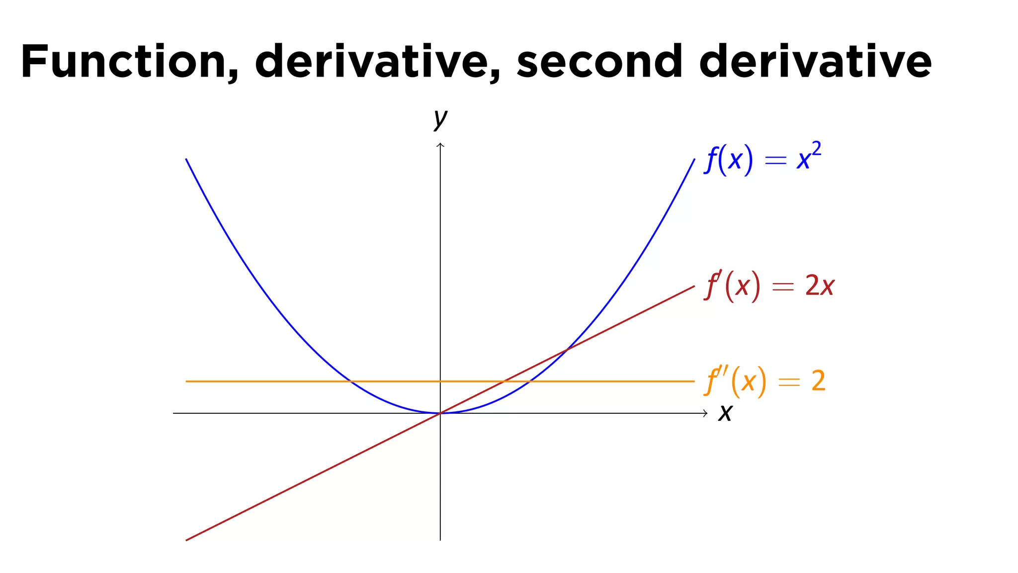
This document outlines the concepts of derivatives in calculus, including the definition, examples, and applications of derivatives in modeling rates of change such as velocity, population growth, and marginal costs. It emphasizes the process of finding derivatives of functions and understanding their graphical representation, along with related tangent problems. Practical examples involving physical rates of change and numerical approximations are also provided to illustrate these concepts.

1. Sec on 2.1–2.2
The Deriva ve
V63.0121.011: Calculus I
Professor Ma hew Leingang
New York University
February 14, 2011
. NYUMathematics

2. Announcements
Quiz this week on
Sec ons 1.1–1.4
No class Monday,
February 21

3. Objectives
The Derivative
Understand and state the defini on of
the deriva ve of a func on at a point.
Given a func on and a point in its
domain, decide if the func on is
differen able at the point and find the
value of the deriva ve at that point.
Understand and give several examples
of deriva ves modeling rates of change
in science.

4. Objectives
The Derivative as a Function
Given a func on f, use the defini on of
the deriva ve to find the deriva ve
func on f’.
Given a func on, find its second
deriva ve.
Given the graph of a func on, sketch
the graph of its deriva ve.

5. Outline
Rates of Change
Tangent Lines
Velocity
Popula on growth
Marginal costs
The deriva ve, defined
Deriva ves of (some) power func ons
What does f tell you about f′ ?
How can a func on fail to be differen able?
Other nota ons
The second deriva ve

6. The tangent problem
A geometric rate of change
Problem
Given a curve and a point on the curve, find the slope of the line
tangent to the curve at that point.

7. A tangent problem
Example
Find the slope of the line tangent to the curve y = x2 at the point
(2, 4).

8. Graphically and numerically
y x2 − 22
x m=
x−2
4
. x
2

9. Graphically and numerically
y x2 − 22
x m=
x−2
3
9
4
. x
2 3

10. Graphically and numerically
y x2 − 22
x m=
x−2
3 5
9
4
. x
2 3

11. Graphically and numerically
y x2 − 22
x m=
x−2
3 5
2.5
6.25
4
. x
2 2.5

12. Graphically and numerically
y x2 − 22
x m=
x−2
3 5
2.5 4.5
6.25
4
. x
2 2.5

13. Graphically and numerically
y x2 − 22
x m=
x−2
3 5
2.5 4.5
2.1
4.41
4
. x
2.1
2

14. Graphically and numerically
y x2 − 22
x m=
x−2
3 5
2.5 4.5
2.1 4.1
4.41
4
. x
2.1
2

15. Graphically and numerically
y x2 − 22
x m=
x−2
3 5
2.5 4.5
2.1 4.1
2.01
4.0401
4
. x
2.01
2

16. Graphically and numerically
y x2 − 22
x m=
x−2
3 5
2.5 4.5
2.1 4.1
2.01 4.01
4.0401
4
. x
2.01
2

17. Graphically and numerically
y x2 − 22
x m=
x−2
3 5
2.5 4.5
2.1 4.1
2.01 4.01
4
1
. x 1
1 2

18. Graphically and numerically
y x2 − 22
x m=
x−2
3 5
2.5 4.5
2.1 4.1
2.01 4.01
4
1
. x 1 3
1 2

19. Graphically and numerically
y x2 − 22
x m=
x−2
3 5
2.5 4.5
2.1 4.1
2.01 4.01
4
2.25
. 1.5
x 1 3
1.5 2

20. Graphically and numerically
y x2 − 22
x m=
x−2
3 5
2.5 4.5
2.1 4.1
2.01 4.01
4
2.25
. 1.5 3.5
x 1 3
1.5 2

21. Graphically and numerically
y x2 − 22
x m=
x−2
3 5
2.5 4.5
2.1 4.1
2.01 4.01
4
3.61
1.9
. 1.5 3.5
x 1 3
1.9
2

22. Graphically and numerically
y x2 − 22
x m=
x−2
3 5
2.5 4.5
2.1 4.1
2.01 4.01
4
3.61
1.9 3.9
. 1.5 3.5
x 1 3
1.9
2

23. Graphically and numerically
y x2 − 22
x m=
x−2
3 5
2.5 4.5
2.1 4.1
2.01 4.01
4
3.9601 1.99
1.9 3.9
. 1.5 3.5
x 1 3
1.99
2

24. Graphically and numerically
y x2 − 22
x m=
x−2
3 5
2.5 4.5
2.1 4.1
2.01 4.01
4
3.9601 1.99 3.99
1.9 3.9
. 1.5 3.5
x 1 3
1.99
2

25. Graphically and numerically
y x2 − 22
x m=
x−2
3 5
2.5 4.5
2.1 4.1
2.01 4.01
4 1.99 3.99
1.9 3.9
. 1.5 3.5
x 1 3
2

26. Graphically and numerically
y x2 − 22
x m=
x−2
3 5
9 2.5 4.5
2.1 4.1
6.25 2.01 4.01
limit
4.41
4.0401
4
3.9601
3.61 1.99 3.99
2.25 1.9 3.9
1 1.5 3.5
. x 1 3
1 1.52.1 3
1.99
2.01
1.92.5
2

27. Graphically and numerically
y x2 − 22
x m=
x−2
3 5
9 2.5 4.5
2.1 4.1
6.25 2.01 4.01
limit 4
4.41
4.0401
4
3.9601
3.61 1.99 3.99
2.25 1.9 3.9
1 1.5 3.5
. x 1 3
1 1.52.1 3
1.99
2.01
1.92.5
2

28. The tangent problem
A geometric rate of change
Problem
Given a curve and a point on the curve, find the slope of the line
tangent to the curve at that point.
Solu on
If the curve is given by y = f(x), and the point on the curve is
(a, f(a)), then the slope of the tangent line is given by
f(x) − f(a)
mtangent = lim
x→a x−a

29. The velocity problem
Kinematics—Physical rates of change
Problem
Given the posi on func on of a moving object, find the velocity of
the object at a certain instant in me.

30. A velocity problem
Example
Drop a ball off the roof of the
Silver Center so that its height can
be described by
h(t) = 50 − 5t2
where t is seconds a er dropping
it and h is meters above the
ground. How fast is it falling one
second a er we drop it?

31. Numerical evidence
h(t) = 50 − 5t2
Fill in the table:
h(t) − h(1)
t vave =
t−1
2 − 15

32. Numerical evidence
h(t) = 50 − 5t2
Fill in the table:
h(t) − h(1)
t vave =
t−1
2 − 15
1.5

33. Numerical evidence
h(t) = 50 − 5t2
Fill in the table:
h(t) − h(1)
t vave =
t−1
2 − 15
1.5 − 12.5

34. Numerical evidence
h(t) = 50 − 5t2
Fill in the table:
h(t) − h(1)
t vave =
t−1
2 − 15
1.5 − 12.5
1.1

35. Numerical evidence
h(t) = 50 − 5t2
Fill in the table:
h(t) − h(1)
t vave =
t−1
2 − 15
1.5 − 12.5
1.1 − 10.5

36. Numerical evidence
h(t) = 50 − 5t2
Fill in the table:
h(t) − h(1)
t vave =
t−1
2 − 15
1.5 − 12.5
1.1 − 10.5
1.01

37. Numerical evidence
h(t) = 50 − 5t2
Fill in the table:
h(t) − h(1)
t vave =
t−1
2 − 15
1.5 − 12.5
1.1 − 10.5
1.01 − 10.05

38. Numerical evidence
h(t) = 50 − 5t2
Fill in the table:
h(t) − h(1)
t vave =
t−1
2 − 15
1.5 − 12.5
1.1 − 10.5
1.01 − 10.05
1.001

39. Numerical evidence
h(t) = 50 − 5t2
Fill in the table:
h(t) − h(1)
t vave =
t−1
2 − 15
1.5 − 12.5
1.1 − 10.5
1.01 − 10.05
1.001 − 10.005

40. A velocity problem
Example Solu on
Drop a ball off the roof of the The answer is
(50 − 5t2 ) − 45
Silver Center so that its height can v = lim
be described by
t→1 t−1
h(t) = 50 − 5t2
where t is seconds a er dropping
it and h is meters above the
ground. How fast is it falling one
second a er we drop it?

41. A velocity problem
Example Solu on
Drop a ball off the roof of the The answer is
(50 − 5t2 ) − 45
Silver Center so that its height can v = lim
be described by
t→1 t−1
5 − 5t2
= lim
h(t) = 50 − 5t2 t→1 t − 1
where t is seconds a er dropping
it and h is meters above the
ground. How fast is it falling one
second a er we drop it?

42. A velocity problem
Example Solu on
Drop a ball off the roof of the The answer is
(50 − 5t2 ) − 45
Silver Center so that its height can v = lim
be described by
t→1 t−1
5 − 5t2
= lim
h(t) = 50 − 5t2 t→1 t − 1
5(1 − t)(1 + t)
where t is seconds a er dropping = lim
t→1 t−1
it and h is meters above the
ground. How fast is it falling one
second a er we drop it?

43. A velocity problem
Example Solu on
Drop a ball off the roof of the The answer is
(50 − 5t2 ) − 45
Silver Center so that its height can v = lim
be described by
t→1 t−1
5 − 5t2
= lim
h(t) = 50 − 5t2 t→1 t − 1
5(1 − t)(1 + t)
where t is seconds a er dropping = lim
t→1 t−1
it and h is meters above the = (−5) lim(1 + t)
t→1
ground. How fast is it falling one
second a er we drop it?

44. A velocity problem
Example Solu on
Drop a ball off the roof of the The answer is
(50 − 5t2 ) − 45
Silver Center so that its height can v = lim
be described by
t→1 t−1
5 − 5t2
= lim
h(t) = 50 − 5t2 t→1 t − 1
5(1 − t)(1 + t)
where t is seconds a er dropping = lim
t→1 t−1
it and h is meters above the = (−5) lim(1 + t)
t→1
ground. How fast is it falling one
second a er we drop it? = −5 · 2 = −10

45. Velocity in general
Upshot
y = h(t)
If the height func on is given h(t0 )
by h(t), the instantaneous ∆h
velocity at me t0 is given by
h(t0 + ∆t)
h(t) − h(t0 )
v = lim
t→t0 t − t0
h(t0 + ∆t) − h(t0 )
= lim
∆t→0 ∆t . ∆t
t
t0 t

46. Population growth
Biological Rates of Change
Problem
Given the popula on func on of a group of organisms, find the rate
of growth of the popula on at a par cular instant.

47. Population growth example
Example
Suppose the popula on of fish in the East River is given by the
func on
3et
P(t) =
1 + et
where t is in years since 2000 and P is in millions of fish. Is the fish
popula on growing fastest in 1990, 2000, or 2010? (Es mate
numerically)

48. Derivation
Solu on
Let ∆t be an increment in me and ∆P the corresponding change in
popula on:
∆P = P(t + ∆t) − P(t)
This depends on ∆t, so ideally we would want
( )
∆P 1 3et+∆t 3et
lim = lim −
∆t→0 ∆t ∆t→0 ∆t 1 + et+∆t 1 + et

49. Derivation
Solu on
Let ∆t be an increment in me and ∆P the corresponding change in
popula on:
∆P = P(t + ∆t) − P(t)
This depends on ∆t, so ideally we would want
( )
∆P 1 3et+∆t 3et
lim = lim −
∆t→0 ∆t ∆t→0 ∆t 1 + et+∆t 1 + et
But rather than compute a complicated limit analy cally, let us
approximate numerically. We will try a small ∆t, for instance 0.1.

50. Numerical evidence
Solu on (Con nued)
To approximate the popula on change in year n, use the difference
P(t + ∆t) − P(t)
quo ent , where ∆t = 0.1 and t = n − 2000.
∆t
r1990
r2000

51. Numerical evidence
Solu on (Con nued)
To approximate the popula on change in year n, use the difference
P(t + ∆t) − P(t)
quo ent , where ∆t = 0.1 and t = n − 2000.
∆t
P(−10 + 0.1) − P(−10)
r1990 ≈
0.1
P(0.1) − P(0)
r2000 ≈
0.1

52. Numerical evidence
Solu on (Con nued)
To approximate the popula on change in year n, use the difference
P(t + ∆t) − P(t)
quo ent , where ∆t = 0.1 and t = n − 2000.
∆t
( )
P(−10 + 0.1) − P(−10) 1 3e−9.9 3e−10
r1990 ≈ = −
0.1 0.1 1 + e−9.9 1 + e−10
( )
P(0.1) − P(0) 1 3e0.1 3e0
r2000 ≈ = −
0.1 0.1 1 + e0.1 1 + e0

53. Numerical evidence
Solu on (Con nued)
To approximate the popula on change in year n, use the difference
P(t + ∆t) − P(t)
quo ent , where ∆t = 0.1 and t = n − 2000.
∆t
( )
P(−10 + 0.1) − P(−10) 1 3e−9.9 3e−10
r1990 ≈ = −
0.1 0.1 1 + e−9.9 1 + e−10
= 0.000143229
( )
P(0.1) − P(0) 1 3e0.1 3e0
r2000 ≈ = −
0.1 0.1 1 + e0.1 1 + e0

54. Numerical evidence
Solu on (Con nued)
To approximate the popula on change in year n, use the difference
P(t + ∆t) − P(t)
quo ent , where ∆t = 0.1 and t = n − 2000.
∆t
( )
P(−10 + 0.1) − P(−10) 1 3e−9.9 3e−10
r1990 ≈ = −
0.1 0.1 1 + e−9.9 1 + e−10
= 0.000143229
( )
P(0.1) − P(0) 1 3e0.1 3e0
r2000 ≈ = −
0.1 0.1 1 + e0.1 1 + e0
= 0.749376

55. Solu on (Con nued)
r2010

56. Solu on (Con nued)
P(10 + 0.1) − P(10)
r2010 ≈
0.1

57. Solu on (Con nued)
( )
P(10 + 0.1) − P(10) 1 3e10.1 3e10
r2010 ≈ = −
0.1 0.1 1 + e10.1 1 + e10

58. Solu on (Con nued)
( )
P(10 + 0.1) − P(10) 1 3e10.1 3e10
r2010 ≈ = −
0.1 0.1 1 + e10.1 1 + e10
= 0.0001296

59. Population growth example
Example
Suppose the popula on of fish in the East River is given by the
func on
3et
P(t) =
1 + et
where t is in years since 2000 and P is in millions of fish. Is the fish
popula on growing fastest in 1990, 2000, or 2010? (Es mate
numerically)
Answer
We es mate the rates of growth to be 0.000143229, 0.749376, and
0.0001296. So the popula on is growing fastest in 2000.

60. Population growth
Biological Rates of Change
Problem
Given the popula on func on of a group of organisms, find the rate
of growth of the popula on at a par cular instant.
Solu on
The instantaneous popula on growth is given by
P(t + ∆t) − P(t)
lim
∆t→0 ∆t

61. Marginal costs
Rates of change in economics
Problem
Given the produc on cost of a good, find the marginal cost of
produc on a er having produced a certain quan ty.

62. Marginal Cost Example
Example
Suppose the cost of producing q tons of rice on our paddy in a year is
C(q) = q3 − 12q2 + 60q
We are currently producing 5 tons a year. Should we change that?

63. Marginal Cost Example
Example
Suppose the cost of producing q tons of rice on our paddy in a year is
C(q) = q3 − 12q2 + 60q
We are currently producing 5 tons a year. Should we change that?
Answer
If q = 5, then C = 125, ∆C = 19, while AC = 25. So we should
produce more to lower average costs.

64. Comparisons
Solu on
C(q) = q3 − 12q2 + 60q
Fill in the table:
q C(q)
4
5
6

65. Comparisons
Solu on
C(q) = q3 − 12q2 + 60q
Fill in the table:
q C(q)
4 112
5
6

66. Comparisons
Solu on
C(q) = q3 − 12q2 + 60q
Fill in the table:
q C(q)
4 112
5 125
6

67. Comparisons
Solu on
C(q) = q3 − 12q2 + 60q
Fill in the table:
q C(q)
4 112
5 125
6 144

68. Comparisons
Solu on
C(q) = q3 − 12q2 + 60q
Fill in the table:
q C(q) AC(q) = C(q)/q
4 112
5 125
6 144

69. Comparisons
Solu on
C(q) = q3 − 12q2 + 60q
Fill in the table:
q C(q) AC(q) = C(q)/q
4 112 28
5 125
6 144

70. Comparisons
Solu on
C(q) = q3 − 12q2 + 60q
Fill in the table:
q C(q) AC(q) = C(q)/q
4 112 28
5 125 25
6 144

71. Comparisons
Solu on
C(q) = q3 − 12q2 + 60q
Fill in the table:
q C(q) AC(q) = C(q)/q
4 112 28
5 125 25
6 144 24

72. Comparisons
Solu on
C(q) = q3 − 12q2 + 60q
Fill in the table:
q C(q) AC(q) = C(q)/q ∆C = C(q + 1) − C(q)
4 112 28
5 125 25
6 144 24

73. Comparisons
Solu on
C(q) = q3 − 12q2 + 60q
Fill in the table:
q C(q) AC(q) = C(q)/q ∆C = C(q + 1) − C(q)
4 112 28 13
5 125 25
6 144 24

74. Comparisons
Solu on
C(q) = q3 − 12q2 + 60q
Fill in the table:
q C(q) AC(q) = C(q)/q ∆C = C(q + 1) − C(q)
4 112 28 13
5 125 25 19
6 144 24

75. Comparisons
Solu on
C(q) = q3 − 12q2 + 60q
Fill in the table:
q C(q) AC(q) = C(q)/q ∆C = C(q + 1) − C(q)
4 112 28 13
5 125 25 19
6 144 24 31

76. Marginal Cost Example
Example
Suppose the cost of producing q tons of rice on our paddy in a year is
C(q) = q3 − 12q2 + 60q
We are currently producing 5 tons a year. Should we change that?
Answer
If q = 5, then C = 125, ∆C = 19, while AC = 25. So we should
produce more to lower average costs.

77. Marginal costs
Rates of change in economics
Problem
Given the produc on cost of a good, find the marginal cost of
produc on a er having produced a certain quan ty.
Solu on
The marginal cost a er producing q is given by
C(q + ∆q) − C(q)
MC = lim
∆q→0 ∆q

78. Outline
Rates of Change
Tangent Lines
Velocity
Popula on growth
Marginal costs
The deriva ve, defined
Deriva ves of (some) power func ons
What does f tell you about f′ ?
How can a func on fail to be differen able?
Other nota ons
The second deriva ve

79. The definition
All of these rates of change are found the same way!

80. The definition
All of these rates of change are found the same way!
Defini on
Let f be a func on and a a point in the domain of f. If the limit
f(a + h) − f(a) f(x) − f(a)
f′ (a) = lim = lim
h→0 h x→a x−a
exists, the func on is said to be differen able at a and f′ (a) is the
deriva ve of f at a.

81. Derivative of the squaring function
Example
Suppose f(x) = x2 . Use the defini on of deriva ve to find f′ (a).

82. Derivative of the squaring function
Example
Suppose f(x) = x2 . Use the defini on of deriva ve to find f′ (a).
Solu on
f(a + h) − f(a)
f′ (a) = lim
h→0 h

83. Derivative of the squaring function
Example
Suppose f(x) = x2 . Use the defini on of deriva ve to find f′ (a).
Solu on
′ f(a + h) − f(a) (a + h)2 − a2
f (a) = lim = lim
h→0 h h→0 h

84. Derivative of the squaring function
Example
Suppose f(x) = x2 . Use the defini on of deriva ve to find f′ (a).
Solu on
′ f(a + h) − f(a) (a + h)2 − a2
f (a) = lim = lim
h→0 h h→0 h
(a + 2ah + h ) − a
2 2 2
= lim
h→0 h

85. Derivative of the squaring function
Example
Suppose f(x) = x2 . Use the defini on of deriva ve to find f′ (a).
Solu on
′ f(a + h) − f(a) (a + h)2 − a2
f (a) = lim = lim
h→0 h h→0 h
(a + 2ah + h ) − a
2 2 2
2ah + h2
= lim = lim
h→0 h h→0 h

86. Derivative of the squaring function
Example
Suppose f(x) = x2 . Use the defini on of deriva ve to find f′ (a).
Solu on
′ f(a + h) − f(a) (a + h)2 − a2
f (a) = lim = lim
h→0 h h→0 h
(a + 2ah + h ) − a
2 2 2
2ah + h2
= lim = lim
h→0 h h→0 h
= lim (2a + h)
h→0

87. Derivative of the squaring function
Example
Suppose f(x) = x2 . Use the defini on of deriva ve to find f′ (a).
Solu on
′ f(a + h) − f(a) (a + h)2 − a2
f (a) = lim = lim
h→0 h h→0 h
(a + 2ah + h ) − a
2 2 2
2ah + h2
= lim = lim
h→0 h h→0 h
= lim (2a + h) = 2a
h→0

88. Derivative of the reciprocal
Example
1
Suppose f(x) = . Use the defini on of the deriva ve to find f′ (2).
x

89. Derivative of the reciprocal
Example
1
Suppose f(x) = . Use the defini on of the deriva ve to find f′ (2).
x
Solu on
y
1/x − 1/2
f′ (2) = lim
x→2 x−2
.
x

90. Derivative of the reciprocal
Example
1
Suppose f(x) = . Use the defini on of the deriva ve to find f′ (2).
x
Solu on
y
1/x − 1/2 2−x
f′ (2) = lim = lim
x→2 x−2 x→2 2x(x − 2)
.
x

91. Derivative of the reciprocal
Example
1
Suppose f(x) = . Use the defini on of the deriva ve to find f′ (2).
x
Solu on
y
1/x − 1/2 2−x
f′ (2) = lim = lim
x→2 x−2 x→2 2x(x − 2)
−1
= lim
x→2 2x
.
x

92. Derivative of the reciprocal
Example
1
Suppose f(x) = . Use the defini on of the deriva ve to find f′ (2).
x
Solu on
y
1/x − 1/2 2−x
f′ (2) = lim = lim
x→2 x−2 x→2 2x(x − 2)
−1 1
= lim =−
x→2 2x 4
.
x

93. “Can you do it the other way?”
Same limit, different form
Solu on
′ f(2 + h) − f(2)
1
2+h− 1
2
f (2) = lim = lim
h→0 h h→0 h

94. “Can you do it the other way?”
Same limit, different form
Solu on
′ f(2 + h) − f(2)
1
2+h− 1
2
f (2) = lim = lim
h→0 h h→0 h
2 − (2 + h)
= lim
h→0 2h(2 + h)

95. “Can you do it the other way?”
Same limit, different form
Solu on
2+h − 2
1 1
′ f(2 + h) − f(2)
f (2) = lim = lim
h→0 h h→0 h
2 − (2 + h) −h
= lim = lim
h→0 2h(2 + h) h→0 2h(2 + h)

96. “Can you do it the other way?”
Same limit, different form
Solu on
2+h − 2
1 1
′ f(2 + h) − f(2)
f (2) = lim = lim
h→0 h h→0 h
2 − (2 + h) −h
= lim = lim
h→0 2h(2 + h) h→0 2h(2 + h)
−1
= lim
h→0 2(2 + h)

97. “Can you do it the other way?”
Same limit, different form
Solu on
2+h − 2
1 1
′ f(2 + h) − f(2)
f (2) = lim = lim
h→0 h h→0 h
2 − (2 + h) −h
= lim = lim
h→0 2h(2 + h) h→0 2h(2 + h)
−1 1
= lim =−
h→0 2(2 + h) 4

98. “How did you get that?”
The Sure-Fire Sally Rule (SFSR) for adding fractions
Fact
a c ad ± bc
± =
b d bd
1 1 2−x
−
x 2 = 2x = 2 − x
x−2 x−2 2x(x − 2)

99. “How did you get that?”
The Sure-Fire Sally Rule (SFSR) for adding fractions
Fact
a c ad ± bc
± =
b d bd
1 1 2−x
−
x 2 = 2x = 2 − x
x−2 x−2 2x(x − 2) Paul Sally

100. What does f tell you about f′?
If f is a func on, we can compute the deriva ve f′ (x) at each
point x where f is differen able, and come up with another
func on, the deriva ve func on.
What can we say about this func on f′ ?

101. What does f tell you about f′?
If f is a func on, we can compute the deriva ve f′ (x) at each
point x where f is differen able, and come up with another
func on, the deriva ve func on.
What can we say about this func on f′ ?
If f is decreasing on an interval, f′ is nega ve (technically, nonposi ve)
on that interval

102. Derivative of the reciprocal
Example
1
Suppose f(x) = . Use the defini on of the deriva ve to find f′ (2).
x
Solu on
y
1/x − 1/2 2−x
f′ (2) = lim = lim
x→2 x−2 x→2 2x(x − 2)
−1 1
= lim =−
x→2 2x 4
.
x

103. What does f tell you about f′?
If f is a func on, we can compute the deriva ve f′ (x) at each
point x where f is differen able, and come up with another
func on, the deriva ve func on.
What can we say about this func on f′ ?
If f is decreasing on an interval, f′ is nega ve (technically, nonposi ve)
on that interval
If f is increasing on an interval, f′ is posi ve (technically, nonnega ve)
on that interval

104. Graphically and numerically
y x2 − 22
x m=
x−2
3 5
9 2.5 4.5
2.1 4.1
6.25 2.01 4.01
limit 4
4.41
4.0401
4
3.9601
3.61 1.99 3.99
2.25 1.9 3.9
1 1.5 3.5
. x 1 3
1 1.52.1 3
1.99
2.01
1.92.5
2

105. What does f tell you about f′?
Fact
If f is decreasing on the open interval (a, b), then f′ ≤ 0 on (a, b).

106. What does f tell you about f′?
Fact
If f is decreasing on the open interval (a, b), then f′ ≤ 0 on (a, b).
Picture Proof.
If f is decreasing, then all secant lines
point downward, hence have y
nega ve slope. The deriva ve is a
limit of slopes of secant lines, which
are all nega ve, so the limit must be
≤ 0. .
x

107. What does f tell you about f′?
Fact
If f is decreasing on on the open interval (a, b), then f′ ≤ 0 on (a, b).
The Real Proof.
If ∆x > 0, then
f(x + ∆x) − f(x)
f(x + ∆x) < f(x) =⇒ <0
∆x

108. What does f tell you about f′?
Fact
If f is decreasing on on the open interval (a, b), then f′ ≤ 0 on (a, b).
The Real Proof.
If ∆x > 0, then
f(x + ∆x) − f(x)
f(x + ∆x) < f(x) =⇒ <0
∆x
If ∆x < 0, then x + ∆x < x, and
f(x + ∆x) − f(x)
f(x + ∆x) > f(x) =⇒ <0
∆x

109. What does f tell you about f′?
Fact
If f is decreasing on on the open interval (a, b), then f′ ≤ 0 on (a, b).
The Real Proof.
f(x + ∆x) − f(x)
Either way, < 0, so
∆x
f(x + ∆x) − f(x)
f′ (x) = lim ≤0
∆x→0 ∆x

110. Going the Other Way?
Ques on
If a func on has a nega ve deriva ve on an interval, must it be
decreasing on that interval?

111. Going the Other Way?
Ques on
If a func on has a nega ve deriva ve on an interval, must it be
decreasing on that interval?
Answer
Maybe.

112. Outline
Rates of Change
Tangent Lines
Velocity
Popula on growth
Marginal costs
The deriva ve, defined
Deriva ves of (some) power func ons
What does f tell you about f′ ?
How can a func on fail to be differen able?
Other nota ons
The second deriva ve

113. Differentiability is super-continuity
Theorem
If f is differen able at a, then f is con nuous at a.

114. Differentiability is super-continuity
Theorem
If f is differen able at a, then f is con nuous at a.
Proof.
We have
f(x) − f(a)
lim (f(x) − f(a)) = lim · (x − a)
x→a x→a x−a
f(x) − f(a)
= lim · lim (x − a)
x→a x−a x→a

115. Differentiability is super-continuity
Theorem
If f is differen able at a, then f is con nuous at a.
Proof.
We have
f(x) − f(a)
lim (f(x) − f(a)) = lim · (x − a)
x→a x→a x−a
f(x) − f(a)
= lim · lim (x − a)
x→a x−a x→a
′
= f (a) · 0

116. Differentiability is super-continuity
Theorem
If f is differen able at a, then f is con nuous at a.
Proof.
We have
f(x) − f(a)
lim (f(x) − f(a)) = lim · (x − a)
x→a x→a x−a
f(x) − f(a)
= lim · lim (x − a)
x→a x−a x→a
′
= f (a) · 0 = 0

117. Differentiability FAIL
Kinks
Example
Let f have the graph on the le -hand side below. Sketch the graph of
the deriva ve f′ .
f(x)
. x

118. Differentiability FAIL
Kinks
Example
Let f have the graph on the le -hand side below. Sketch the graph of
the deriva ve f′ .
f(x) f′ (x)
. x . x

119. Differentiability FAIL
Kinks
Example
Let f have the graph on the le -hand side below. Sketch the graph of
the deriva ve f′ .
f(x) f′ (x)
. x . x

120. Differentiability FAIL
Cusps
Example
Let f have the graph on the le -hand side below. Sketch the graph of
the deriva ve f′ .
f(x)
. x

121. Differentiability FAIL
Cusps
Example
Let f have the graph on the le -hand side below. Sketch the graph of
the deriva ve f′ .
f(x) f′ (x)
. x . x

122. Differentiability FAIL
Cusps
Example
Let f have the graph on the le -hand side below. Sketch the graph of
the deriva ve f′ .
f(x) f′ (x)
. x . x

123. Differentiability FAIL
Cusps
Example
Let f have the graph on the le -hand side below. Sketch the graph of
the deriva ve f′ .
f(x) f′ (x)
. x . x

124. Differentiability FAIL
Vertical Tangents
Example
Let f have the graph on the le -hand side below. Sketch the graph of
the deriva ve f′ .
f(x)
. x

125. Differentiability FAIL
Vertical Tangents
Example
Let f have the graph on the le -hand side below. Sketch the graph of
the deriva ve f′ .
f(x) f′ (x)
. x . x

126. Differentiability FAIL
Vertical Tangents
Example
Let f have the graph on the le -hand side below. Sketch the graph of
the deriva ve f′ .
f(x) f′ (x)
. x . x

127. Differentiability FAIL
Vertical Tangents
Example
Let f have the graph on the le -hand side below. Sketch the graph of
the deriva ve f′ .
f(x) f′ (x)
. x . x

128. Differentiability FAIL
Weird, Wild, Stuff
Example
f(x)
. x
This func on is differen able
at 0.

129. Differentiability FAIL
Weird, Wild, Stuff
Example
f(x) f′ (x)
. x . x
This func on is differen able
at 0.

130. Differentiability FAIL
Weird, Wild, Stuff
Example
f(x) f′ (x)
. x . x
This func on is differen able
at 0.

131. Differentiability FAIL
Weird, Wild, Stuff
Example
f(x) f′ (x)
. x . x
This func on is differen able But the deriva ve is not
at 0. con nuous at 0!

132. Outline
Rates of Change
Tangent Lines
Velocity
Popula on growth
Marginal costs
The deriva ve, defined
Deriva ves of (some) power func ons
What does f tell you about f′ ?
How can a func on fail to be differen able?
Other nota ons
The second deriva ve

133. Notation
Newtonian nota on
f′ (x) y′ (x) y′
Leibnizian nota on
dy d df
f(x)
dx dx dx
These all mean the same thing.

134. Meet the Mathematician
Isaac Newton
English, 1643–1727
Professor at Cambridge
(England)
Philosophiae Naturalis
Principia Mathema ca
published 1687

135. Meet the Mathematician
Gottfried Leibniz
German, 1646–1716
Eminent philosopher as
well as mathema cian
Contemporarily disgraced
by the calculus priority
dispute

136. Outline
Rates of Change
Tangent Lines
Velocity
Popula on growth
Marginal costs
The deriva ve, defined
Deriva ves of (some) power func ons
What does f tell you about f′ ?
How can a func on fail to be differen able?
Other nota ons
The second deriva ve

137. The second derivative
If f is a func on, so is f′ , and we can seek its deriva ve.
f′′ = (f′ )′
It measures the rate of change of the rate of change!

138. The second derivative
If f is a func on, so is f′ , and we can seek its deriva ve.
f′′ = (f′ )′
It measures the rate of change of the rate of change! Leibnizian
nota on:
d2 y d2 d2 f
f(x)
dx2 dx2 dx2

139. Function, derivative, second derivative
y
f(x) = x2
f′ (x) = 2x
f′′ (x) = 2
. x

140. Summary
What have we learned today?
The deriva ve measures instantaneous rate of change
The deriva ve has many interpreta ons: slope of the tangent
line, velocity, marginal quan es, etc.
The deriva ve reflects the monotonicity (increasing-ness or
decreasing-ness) of the graph