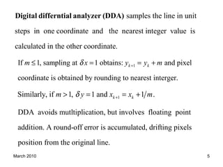
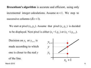
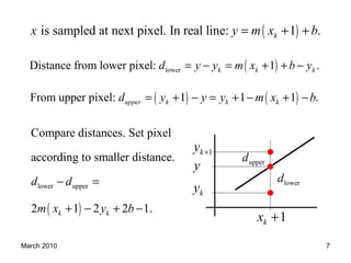
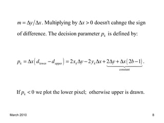
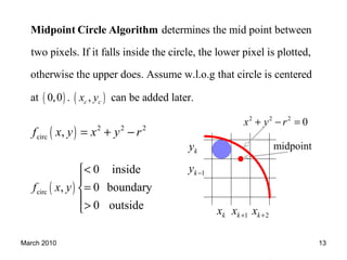
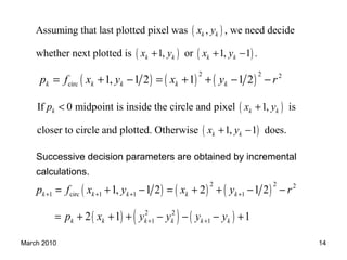
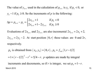
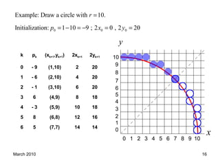
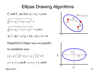
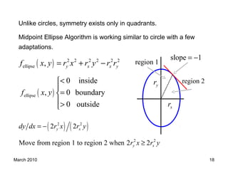
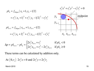
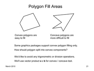
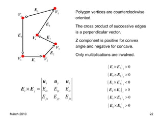
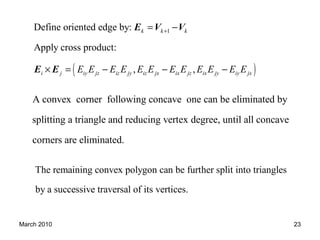
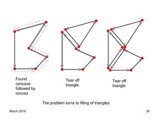
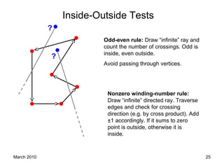
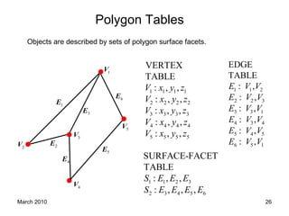
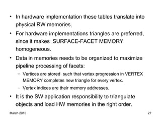
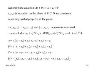
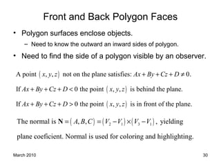
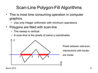
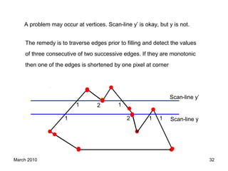
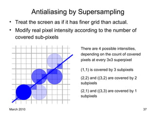
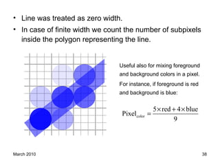
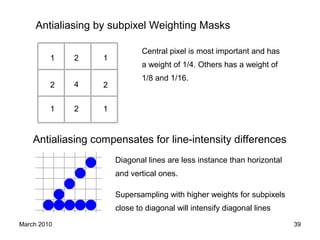
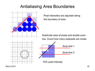
SlideShare a Scribd company logo
March 2010 1
Shape Drawing Algorithms
Shmuel Wimer
Bar Ilan Univ., Engineering Faculty
March 2010 2
Display
Window
maxy
miny
minx
maxx
World –coordinate limits
y
x0
1
2
3
4
5
0 1 2 3 4 5
Screen –coordinates
(4,2) pixel
coordinate
March 2010 3
We’d like to display straight line on the screen.
On raster systems, lines are plotted with pixels which have vertical
and horizontal finite resolution.
The outcome is a jaggy line.
In analog displays, such as vector-scan, a smooth line can be
displayed, as line equation is translated into deflection voltages.
Line Drawing Algorithms
March 2010 4
straight line equation: y mx b= +
0x
0y
endx
endy
end 0
0 0
end 0
;
y y
m b y mx
x x
−
= = −
−
Straight line drawing uses increments or and finds the
counterpart. If | | 1 , and if | | 1 .
x y
m y m x m x y m
δ δ
δ δ δ δ≤ = > =
In raster systems lines are plotted with pixels and step sizes in the
horizontal and vertical directions must be sampled at nearest pixel
positions.
March 2010 5
1If 1, sampling at 1 obtains: and pixel
coordinate is obtained by rounding to nearest interger.
k km x y y mδ +≤ = = +
samples the line in unit
steps in one coordinate and the nearest integer value is
calculated in the other coordinate.
Digital differntial analyzer (DDA)
1Similarly, if 1, 1 and 1 .k km y x x mδ +> = = +
DDA avoids mutltiplication, but involves floating point
addition. A round-off error is accumulated, drifting pixels
position from the original line.
March 2010 6
is accurate and efficient, using only
incremental integer calculations. Assume 1. We step to
successive columns ( 1).
m
xδ
<
=
Bresenham's algorithm
0 0
1
We start at pixel ( ,y ). Assume that pixel ( ,y ) is decided
to be displayed. Next pixel is either ( +1,y ) or ( +1,y ).
k k
k k k k
x x
x x +
1Decision on or is
made according to which
one is closer to the real
of the line.
k ky y
y
+
ky
y
1ky +
1kx +
March 2010 7
( )is sampled at next pixel. In real line: 1 .kx y m x b= + +
( )lowerDistance from lower pixel: 1 .k k kd y y m x b y= − = + + −
( ) ( )From upper pixel: 1 1 1 .upper k k kd y y y m x b= + − = + − + −
( )
lower upper
Compare distances. Set pixel
according to smaller distance.
2 1 2 2 1.k k
d d
m x y b
− =
+ − + −
ky
y
1ky +
1kx +
lowerd
upperd
March 2010 8
. Multiplying by 0 doesn't cahnge the sign
of difference. The decision parameter is defined by:k
m y x x
p
= ∆ ∆ ∆ >
( ) ( )lower upper
constant
2 2 2 2 1 .k k kp x d d x y y x y x b= ∆ − = ∆ − ∆ + ∆ + ∆ −
1442443
If 0 we plot the lower pixel; otherwise upper is drawn.kp <
March 2010 9
( ) ( )
( )
1 1 1
1
2 2
0 if 0
2 2 2 .
2 if 0
k k k k k k
k
k k
k
p p y x x x y y
p
y x y y y
x p
+ + +
+
− = ∆ − − ∆ − =
>
∆ − ∆ − = ∆ − 
∆ ≤
( )1 1 1
constant
The decision can be computed recursively as follows:
2 2 2 2 1 .
k
k k k
p
p y x x y y x b+ + += ∆ × − ∆ × + ∆ + ∆ −
1442443
March 2010 10
Circle Drawing Algorithms
( ),x y
θ
cx
cy
r
( ) ( )2 2 2
c cx x y y r− + − =
We could use above equation to
step along the x axis from xc- r
to xc+ r and calculate y positions
of pixels.
( )
22
c cy y r x x= ± − −
March 2010 11
This requires considerable amount of computation (square root)
The drawing appearance is poor since the vertical spacing
between drawn pixels is uneven.
Appearance can be improved by changing the role of x and y
whenever the absolute value of the slope of circle is crossing 1.
But this requires more computation.
Polar coordinates can be used with
uniform stepping of θ. This spaces
pixels evenly along circumference.
cos
sin
c
c
x x r
y y r
θ
θ
= +
= +
Time consuming due to trigonometric computations.
March 2010 12
We can use large angular steps and
connect the points by straight lines.
For smoother boundary we can use
angular steps of 1/r which plots
pixels approximately one pixel
apart of each other (r∙1/r =1).
O
45
( ),x y
( ),x y−
( ),x y−
( ),x y− −
( ),y x− ( ),y x
( ),y x− − ( ),y x−
Any of the methods can use
symmetry for efficiency.
All methods involve
expensive computations.
March 2010 13
( )
determines the mid point between
two pixels. If it falls inside the circle, the lower pixel is plotted,
otherwise the upper does. Assume w.l.o.g that circle is centered
at 0,0 .
Midpoint Circle Algorithm
( ), can be added later.c cx y
( ) 2 2 2
circ ,f x y x y r= + −
( )circ
0 inside
, 0 boundary
0 outside
f x y
<

=
>
ky
1ky −
2kx +1kx +kx
midpoint
2 2 2
0x y r+ − =
March 2010 14
Successive decision parameters are obtained by incremental
calculations.
( ) ( ) ( )
2 2 2
circ 1, 1 2 1 1 2k k k k kp f x y x y r= + − = + + − −
( )
( ) ( )
Assuming that last plotted pixel was , , we need decide
whether next plotted is 1, or 1, 1 .
k k
k k k k
x y
x y x y+ + −
( )
( )
If 0 midpoint is inside the circle and pixel 1, is
closer to circle and plotted. Otherwise 1, 1 does.
k k k
k k
p x y
x y
< +
+ −
( ) ( ) ( )
( ) ( ) ( )
2 2 2
1 circ 1 1 1
2 2
1 1
1, 1 2 2 1 2
2 1 1
k k k k k
k k k k k k
p f x y x y r
p x y y y y
+ + + +
+ +
= + − = + + − −
= + + + − − − +
March 2010 15
1 1
1
1
1 1
The value of used in the calculation of is if 0, or
1 if 0. So the increments of is the following:
2 1 if 0
2 1 2 if 0
k k k k
k k
k k
k k
k k k
y p y p
y p p
x p
p p p
x y p
+ +
+
+
+ +
<
− ≥
+ <
∆ = − = 
+ − ≥
( )
1 1 1
1
Evaluations of 2 and 2 are also incremental 2 2 2,
2 2 2. At start position 0, these values are 0 and 2 ,
respectively.
k k k k
k k
x y x x
y y r r
+ + +
+
= +
= −
( ) ( ) ( )
( )
0 0 0 0 circ
2 2
0
is obtained from , 0, , 1, 1 2
1 1 2 5 4 . updates are made by integral
increments and decrements, so if is integer, we set 1 .
p x y r p f r
r r r p
r p r
= = −
= + − − = −
= −
March 2010 16
y
x
1 2 3 4 5 6 7 8 90 10
1
2
3
8
9
0
10
5
6
7
4
k pk (xk+1,yk+1) 2xk+1 2yk+1
0 - 9 (1,10) 2 20
1 - 6 (2,10) 4 20
2 - 1 (3,10) 6 20
3 6 (4,9) 8 18
4 - 3 (5,9) 10 18
5 8 (6,8) 12 16
6 5 (7,7) 14 14
0 0 0
Example: Draw a circle with 10.
Initialization: 1 10 9 ; 2 0 , 2 20
r
p x y
=
= − = − = =
March 2010 17cx
cy
yr
xr
Ellipse Drawing Algorithms
1F
2F
1d
2d
( ),P x y=
( ) ( )
( ) ( )
1 2 1 2
2 2
1 1
2 2
2 2
2 2
and are foci,
0
F F d d const
x x y y
x x y y const
Ax By Cxy Dx Ey F
+ =
− + − +
− + − =
+ + + + + =
( ) ( )
2 22 2
Simplified if ellipse axes are parallel
to coordinate axes.
1
cos ; sin
c x c y
c x c y
x x r y y r
x x r y y rθ θ
− + − =
= + = +
March 2010 18
Unlike circles, symmetry exists only in quadrants.
Midpoint Ellipse Algorithm is working similar to circle with a few
adaptations.
( ) 2 2 2 2 2 2
ellipse , y x x yf x y r x r y r r= + −
( )ellipse
0 inside
, 0 boundary
0 outside
f x y
<

=
>
slope 1= −
yr
xr
region 1
region 2
( ) ( )2 2
2 2
2 2
Move from region 1 to region 2 when 2 2
y x
y x
dy dx r x r y
r x r y
= −
≥
March 2010 19
ky
1ky −
2kx +1kx +kx
midpoint
2 2 2 2 2 2
0y x x yr x r y r r+ − =
( )
( ) ( )
ellipse
2 22 2 2 2
1 1, 1 2
1 1 2
k k k
y k x k x y
p f x y
r x r y r r
= + −
= + + − −
( )
( ) ( )
1 ellipse 1 1
2 22 2 2 2
1
1 1, 1 2
2 1 2
k k k
y k x k x y
p f x y
r x r y r r
+ + +
+
= + −
= + + − −
( )
2 2
1
1 2 2 2
1 1
2 2 2
2 if 1 0
1 1
2 2 if 1 0
These terms can be calculated by addition only.
At 0, 2 0 and 2 2
y k y k
k k
y k y x k k
y y x x y
r x r p
p p p
r x r r y p
r r x r y r r
+
+
+ +
 + <
∆ = − = 
+ − ≥
= =
March 2010 20
( ) ( )
( )
0 0 0
2 2 2
0 ellipse
1 is obtained from , 0, ,
1 1, 1 2 4.
y
y y x y x
p x y r
p f r r r r r
=
= − = − +
( ) ( )0 0
2 is handled similarly. We could start at the end point
of region1 and proceed clockwise, but it is better to walk
counterclockwise, starting at , ,0 .
k
x
p
x y r=
March 2010 21
Polygon Fill Areas
Convex polygons are
easy to fill
Concave polygons are
more difficult to fill
Some graphics packages support convex polygon filling only.
How should polygon split into convex components?
We’d like to avoid any trigonometric or division operations.
We’ll use vector product a x b for convex / concave test.
March 2010 22
( )1 2 0z
× >E E
( )2 3 0z
× >E E
( )3 4 0z
× <E E
( )4 5 0z
× >E E
( )5 6 0z
× >E E
( )6 1 0z
× >E E
1E1V 2V
3V
5V
6V
4V
2E
3E
4E
5E
6E
x y z
i j ix iy iz
jx jy jz
E E E
E E E
× =
u u u
E E
Polygon vertices are counterclockwise
oriented.
The cross product of successive edges
is a perpendicular vector.
Z component is positive for convex
angle and negative for concave.
Only multiplications are involved.
March 2010 23
( )
1Define oriented edge by:
Apply cross product:
, ,
k k k
i j iy jz iz jy iz jx ix jz ix jy iy jxE E E E E E E E E E E E
+= −
× = − − −
E V V
E E
A convex corner following concave one can be eliminated by
splitting a triangle and reducing vertex degree, until all concave
corners are eliminated.
The remaining convex polygon can be further split into triangles
by a successive traversal of its vertices.
March 2010 24
The problem turns to filling of triangles
Found
concave
followed by
convex
Tear off
triangle
Tear off
triangle
March 2010 25
Inside-Outside Tests
?
Odd-even rule: Draw “infinite” ray and
count the number of crossings. Odd is
inside, even outside.
Avoid passing through vertices.
?
Nonzero winding-number rule:
Draw “infinite” directed ray. Traverse
edges and check for crossing
direction (e.g. by cross product). Add
±1 accordingly. If it sums to zero
point is outside, otherwise it is
inside.
March 2010 26
Polygon Tables
Objects are described by sets of polygon surface facets.
1E
1V
2V
3V
5V
4V
2E
3E
4E
5E
6E
1 1 1 1
2 2 2 2
3 3 3 3
4 4 4 4
5 5 5 5
VERTEX
TABLE
: , ,
: , ,
: , ,
: , ,
: , ,
V x y z
V x y z
V x y z
V x y z
V x y z
1 1 2
2 2 3
3 3 1
4 3 4
5 4 5
6 5 1
EDGE
TABLE
: ,
: ,
: ,
: ,
: ,
: ,
E V V
E V V
E V V
E V V
E V V
E V V
1 1 2 3
2 3 4 5 6
SURFACE-FACET
TABLE
: , ,
: , , ,
S E E E
S E E E E
March 2010 27
• In hardware implementation these tables translate into
physical RW memories.
• For hardware implementations triangles are preferred,
since it makes SURFACE-FACET MEMORY
homogeneous.
• Data in memories needs to be organized to maximize
pipeline processing of facets:
– Vertices are stored such that vertex progression in VERTEX
MEMORY completes new triangle for every vertex.
– Vertex indices are their memory addresses.
• It is the SW application responsibility to triangulate
objects and load HW memories in the right order.
March 2010 28
Plane Equations
• Graphics system processes input data through several
steps:
– Transformation of modeling through viewing pipeline.
– Identification of visible surfaces.
– Rendering of surface facets.
• Information about the spatial orientation of surfaces is
needed
– Plane equations are in order.
– How to calculate those efficiently w/o divisions?
March 2010 29
General plane equation: 0
, , is any point on the plane. , , , are constansts
describing spatial propertis of the plane.
Ax By Cz D
x y z A B C D
+ + + =
( ) ( ) ( )
( ) ( ) ( )
1 1 1 2 2 2 3 3 3, , , , , and , , non co-linear ordered
counterclockwise, 1, 1,2,3.k k k
x y z x y z x y z
A D x B D y C D z k+ + = − =
( ) ( ) ( )
( ) ( ) ( )
( ) ( ) ( )
( ) ( ) ( )
1 2 3 2 3 1 3 1 2
1 2 3 2 3 1 3 1 2
1 2 3 2 3 1 3 1 2
1 2 3 3 2 2 3 1 1 3 3 1 2 2 1
A y z z y z z y z z
B z x x z x x z x x
C x y y x y y x y y
D x y z y z x y z y z x y z y z
= − + − + −
= − + − + −
= − + − + −
= − − + − + −  
March 2010 30
Front and Back Polygon Faces
• Polygon surfaces enclose objects.
– Need to know the outward an inward sides of polygon.
• Need to find the side of a polygon visible by an observer.
( )
( )
( )
A point , , not on the plane satisfies: 0.
If 0 the point , , is behind the plane.
If 0 the point , , is in front of the plane.
x y z Ax By Cz D
Ax By Cz D x y z
Ax By Cz D x y z
+ + + ≠
+ + + <
+ + + >
( ) ( ) ( )2 1 3 1The normal is , , , yielding
plane coeficient. Normal is used for coloring and highlighting.
A B C V V V V= = − × −N
March 2010 31
Scan-Line Polygon-Fill Algorithms
• This is most time consuming operation in computer
graphics.
– Use only integer arithmetic with minimum operations
• Polygons are filled with scan-line
– The sweep is vertical
– A scan-line is the pixels of same y coordinates
Pixels between odd-even
intersections with border
are inside.
y
x
1 2 3 4
March 2010 32
11 12 Scan-line y
21 1
Scan-line y’
A problem may occur at vertices. Scan-line y’ is okay, but y is not.
The remedy is to traverse edges prior to filling and detect the values
of three consecutive of two successive edges. If they are monotonic
then one of the edges is shortened by one pixel at corner
March 2010 33
Polygon filling takes advantage of y increments by one unit.
( ),k kx y
( )1 1,k kx y+ + Scan-line 1ky +
Scan-line ky
How to calculate efficiently the intersection of an edge with scan line?
( )
( )
1
1 1
1
1
, 1k k
k k k k
k k
y y
m y y x x
x x m
+
+ +
+
−
= = + ⇒ = +
−
How to avoid division?
March 2010 34
1Calculate interceps by: , k k
y x
x m x x
x y
+
∆ ∆
= = +
∆ ∆
Initialize a counter to 0. Then increment the counter by each time
is incremented by 1 (moving to new scal-line). Once counter meets
or exceeds , is increased by 1 and counter is decreased b
x
y
y x
∆
∆ y .y∆
This is equivalent to maintaining integer and fractional parts of
intercepts and incrementing the fractional parts until it reaches
the next integer value.
March 2010 35
Instead of truncation we can round to nearest pixel intersection
by comparing the counter to 2. This can be done with integer
arithmetics by adding 2 , comparing to , and then decreasing
counter
x
y
x y
∆
∆ ∆
by 2 .y∆
( ) ( ) ( )
( ) ( ) ( ) ( )
( ) ( )
0 0 0 0
0 0 0 0 0 0 0
0 0 0
Example: 7 3. , : ,0 : , 1,3 : ,
2,6 : , 3,9 3,2 : 1, 4,5 : 1,
5,8 5,1 : 2,...
y x y count x y x y x
y x y y x y x
y y x
∆ ∆ = = +
+ + → + + + +
+ → + +
( ) ( ) ( )
( ) ( ) ( ) ( )
( )
0 0 0 0
0 0 0 0 0 0
0 0
Example: 7 3. , : ,0 : , 1,6 : ,
2,12 2, 2 : 1, 3,4 : 1, 4,10
4, 4 : 2,...
y x y count x y x y x
y y x y x y
y x
∆ ∆ = = +
+ → + − + + + + →
+ − +
March 2010 36
Antialiasing
• Graphics primitives generated by raster algorithms have
jagged (stair-step) appearance, called aliasing.
– This is due to under sampling.
– Antialiasing compensates for this.
• Sampling rate could increase by higher raster resolution.
– Expensive, increase of frame buffer (memory).
– More processing (time, hardware).
– Jagging phenomena is not canceled, but only improved.
• Raster systems capable of gradual intensity of pixels can
support antialiasing by modifying pixel intensity near
boundary of primitives.
March 2010 37
Antialiasing by Supersampling
• Treat the screen as if it has finer grid than actual.
• Modify real pixel intensity according to the number of
covered sub-pixels
There are 4 possible intensities,
depending on the count of covered
pixels at every 3x3 superpixel
(1,1) is covered by 3 subpixels
(2,2) and ((3,2) are covered by 2
subpixels
(2,1) and ((3,3) are covered by 1
subpixels
March 2010 38
• Line was treated as zero width.
• In case of finite width we count the number of subpixels
inside the polygon representing the line.
Useful also for mixing foreground
and background colors in a pixel.
For instance, if foreground is red
and background is blue:
color
5 red 4 blue
Pixel
9
× + ×
=
March 2010 39
1
1
1
1
2
2
2 24
Central pixel is most important and has
a weight of 1/4. Others has a weight of
1/8 and 1/16.
Antialiasing by subpixel Weighting Masks
Antialiasing compensates for line-intensity differences
Diagonal lines are less instance than horizontal
and vertical ones.
Supersampling with higher weights for subpixels
close to diagonal will intensify diagonal lines
March 2010 40
Antialiasing Area Boundaries
Pixel intensities are adjusted along
the boundary of area.
Subdivide area of pixels and double scan-
line. Count how many subpixels are inside.
Scan-line 1
Scan-line 2
75% pixel intensity
March 2010 41
Percentage of pixel area within fill area by midpoint
method (Pitteway & Watkinson).
ky
0.5ky +
1ky +
kx 1kx +
y mx b= +
( )
1
Assume that , has been
plotted. The next nearest
line at is either at or at
1.
k k
k k
k
x y
x y
y
+
+
( ) ( )mid
if 0 select 1
1 0.5 ,
if 0 select
or by adding the term 1
k
k k
k
y
y y m x b y
y
m
> +
− = + + − +    <
−
( ) ( ) ( )
if 1 select 1
1 0.5 1
if 1 select
k
k k
k
m y
p m x b y m
m y
> − +
= + + − + + −    < −
March 2010 42
0.5kx +0.5kx − kx
0.5ky +
0.5ky −
ky
( )0.5ky m x b= − + ( )0.5ky m x b= + +
boundary line
overlap area
( )The overlap area of a pixel rectangle at , with the interior
of polygon is: area 0.5 .
We can intensify the pixel for antialiasing accordingly.
k k
k k
x y
mx b y p= + − + =

More Related Content

What's hot

Computer graphics - bresenham line drawing algorithm
Computer graphics - bresenham line drawing algorithmComputer graphics - bresenham line drawing algorithm
Computer graphics - bresenham line drawing algorithm
Ruchi Maurya
 
1603 plane sections of real and complex tori
1603 plane sections of real and complex tori1603 plane sections of real and complex tori
1603 plane sections of real and complex tori
Dr Fereidoun Dejahang
 
Transformations (complex variable & numerical method)
Transformations (complex variable & numerical method)Transformations (complex variable & numerical method)
Transformations (complex variable & numerical method)
Digvijaysinh Gohil
 
U unit4 vm
U unit4 vmU unit4 vm
U unit4 vm
Akhilesh Deshpande
 
graphs of functions 2
 graphs of functions 2 graphs of functions 2
graphs of functions 2larasati06
 
Exam ii(practice)
Exam ii(practice)Exam ii(practice)
Exam ii(practice)PublicLeaks
 
Higher papers 2007 - 2013
Higher papers 2007 -  2013Higher papers 2007 -  2013
Higher papers 2007 - 2013
sjamaths
 
Kem akademik sept 16
Kem akademik  sept 16Kem akademik  sept 16
Kem akademik sept 16
SMK Mukah
 
Numerical Methods: curve fitting and interpolation
Numerical Methods: curve fitting and interpolationNumerical Methods: curve fitting and interpolation
Numerical Methods: curve fitting and interpolation
Nikolai Priezjev
 
1627 simultaneous equations and intersections
1627 simultaneous equations and intersections1627 simultaneous equations and intersections
1627 simultaneous equations and intersections
Dr Fereidoun Dejahang
 
H 2004 2007
H 2004   2007H 2004   2007
H 2004 2007
sjamaths
 
Clase funcion cuadratica
Clase funcion cuadraticaClase funcion cuadratica
Clase funcion cuadraticasainpereztorres
 
Exams in college algebra
Exams in college algebraExams in college algebra
Exams in college algebra
Raymond Garcia
 
Calculo integral - Larson
Calculo integral - LarsonCalculo integral - Larson
Calculo integral - Larson
Juan Alejandro Alvarez Agudelo
 
Trial spm smk_st_george_taiping_2013_maths_paper1_2_[a]
Trial spm smk_st_george_taiping_2013_maths_paper1_2_[a]Trial spm smk_st_george_taiping_2013_maths_paper1_2_[a]
Trial spm smk_st_george_taiping_2013_maths_paper1_2_[a]
Karthik Karunanithy
 
U unit3 vm
U unit3 vmU unit3 vm
U unit3 vm
Akhilesh Deshpande
 
Foundation c2 exam august 2012 sols
Foundation c2 exam august 2012 solsFoundation c2 exam august 2012 sols
Foundation c2 exam august 2012 solsfatima d
 
Jacobi method
Jacobi methodJacobi method
Jacobi method
Grishma Maravia
 

What's hot (19)

Computer graphics - bresenham line drawing algorithm
Computer graphics - bresenham line drawing algorithmComputer graphics - bresenham line drawing algorithm
Computer graphics - bresenham line drawing algorithm
 
1603 plane sections of real and complex tori
1603 plane sections of real and complex tori1603 plane sections of real and complex tori
1603 plane sections of real and complex tori
 
Transformations (complex variable & numerical method)
Transformations (complex variable & numerical method)Transformations (complex variable & numerical method)
Transformations (complex variable & numerical method)
 
U unit4 vm
U unit4 vmU unit4 vm
U unit4 vm
 
graphs of functions 2
 graphs of functions 2 graphs of functions 2
graphs of functions 2
 
Exam ii(practice)
Exam ii(practice)Exam ii(practice)
Exam ii(practice)
 
Higher papers 2007 - 2013
Higher papers 2007 -  2013Higher papers 2007 -  2013
Higher papers 2007 - 2013
 
1301 c1 january_2013_mark_scheme
1301 c1 january_2013_mark_scheme1301 c1 january_2013_mark_scheme
1301 c1 january_2013_mark_scheme
 
Kem akademik sept 16
Kem akademik  sept 16Kem akademik  sept 16
Kem akademik sept 16
 
Numerical Methods: curve fitting and interpolation
Numerical Methods: curve fitting and interpolationNumerical Methods: curve fitting and interpolation
Numerical Methods: curve fitting and interpolation
 
1627 simultaneous equations and intersections
1627 simultaneous equations and intersections1627 simultaneous equations and intersections
1627 simultaneous equations and intersections
 
H 2004 2007
H 2004   2007H 2004   2007
H 2004 2007
 
Clase funcion cuadratica
Clase funcion cuadraticaClase funcion cuadratica
Clase funcion cuadratica
 
Exams in college algebra
Exams in college algebraExams in college algebra
Exams in college algebra
 
Calculo integral - Larson
Calculo integral - LarsonCalculo integral - Larson
Calculo integral - Larson
 
Trial spm smk_st_george_taiping_2013_maths_paper1_2_[a]
Trial spm smk_st_george_taiping_2013_maths_paper1_2_[a]Trial spm smk_st_george_taiping_2013_maths_paper1_2_[a]
Trial spm smk_st_george_taiping_2013_maths_paper1_2_[a]
 
U unit3 vm
U unit3 vmU unit3 vm
U unit3 vm
 
Foundation c2 exam august 2012 sols
Foundation c2 exam august 2012 solsFoundation c2 exam august 2012 sols
Foundation c2 exam august 2012 sols
 
Jacobi method
Jacobi methodJacobi method
Jacobi method
 

Similar to Shape drawing algs

Lines and curves algorithms
Lines and curves algorithmsLines and curves algorithms
Lines and curves algorithmsMohammad Sadiq
 
Computer_Graphics_circle_drawing_techniq.ppt
Computer_Graphics_circle_drawing_techniq.pptComputer_Graphics_circle_drawing_techniq.ppt
Computer_Graphics_circle_drawing_techniq.ppt
AliZaib71
 
10994479.ppt
10994479.ppt10994479.ppt
10994479.ppt
ALIZAIB KHAN
 
Computer Graphics Unit 2
Computer Graphics Unit 2Computer Graphics Unit 2
Computer Graphics Unit 2
SanthiNivas
 
maths jee formulas.pdf
maths jee formulas.pdfmaths jee formulas.pdf
maths jee formulas.pdf
GARRYB4
 
Output Primitives in Computer Graphics and Multimedia
Output Primitives in Computer Graphics and MultimediaOutput Primitives in Computer Graphics and Multimedia
Output Primitives in Computer Graphics and Multimedia
saranyan75
 
Computer Graphics and Multimedia Output primitives
Computer Graphics and Multimedia Output primitivesComputer Graphics and Multimedia Output primitives
Computer Graphics and Multimedia Output primitives
saranyan75
 
Spm add-maths-formula-list-form4-091022090639-phpapp01
Spm add-maths-formula-list-form4-091022090639-phpapp01Spm add-maths-formula-list-form4-091022090639-phpapp01
Spm add-maths-formula-list-form4-091022090639-phpapp01
Asad Bukhari
 
Spm add-maths-formula-list-form4-091022090639-phpapp01
Spm add-maths-formula-list-form4-091022090639-phpapp01Spm add-maths-formula-list-form4-091022090639-phpapp01
Spm add-maths-formula-list-form4-091022090639-phpapp01
Nur Kamila
 
Additional Mathematics form 4 (formula)
Additional Mathematics form 4 (formula)Additional Mathematics form 4 (formula)
Additional Mathematics form 4 (formula)
Fatini Adnan
 
Unit 3
Unit 3Unit 3
TABREZ KHAN.ppt
TABREZ KHAN.pptTABREZ KHAN.ppt
TABREZ KHAN.ppt
TabrezKhan733764
 
Output Primitive and Brenshamas Line.pptx
Output Primitive and Brenshamas Line.pptxOutput Primitive and Brenshamas Line.pptx
Output Primitive and Brenshamas Line.pptx
NaveenaKarthik3
 
IIT Jam math 2016 solutions BY Trajectoryeducation
IIT Jam math 2016 solutions BY TrajectoryeducationIIT Jam math 2016 solutions BY Trajectoryeducation
IIT Jam math 2016 solutions BY Trajectoryeducation
Dev Singh
 
2D Geometry1
2D Geometry12D Geometry1
Solucao_Marion_Thornton_Dinamica_Classic (1).pdf
Solucao_Marion_Thornton_Dinamica_Classic (1).pdfSolucao_Marion_Thornton_Dinamica_Classic (1).pdf
Solucao_Marion_Thornton_Dinamica_Classic (1).pdf
FranciscoJavierCaedo
 
Computer graphics 2
Computer graphics 2Computer graphics 2
Computer graphics 2
Prabin Gautam
 
Dda algo notes
Dda algo notesDda algo notes
Dda algo notes
shreeja asopa
 
Test yourself for JEE(Main)TP-5
Test yourself for JEE(Main)TP-5Test yourself for JEE(Main)TP-5
Test yourself for JEE(Main)TP-5
Vijay Joglekar
 
Chapter 3 Output Primitives
Chapter 3 Output PrimitivesChapter 3 Output Primitives
Chapter 3 Output Primitives
PrathimaBaliga
 

Similar to Shape drawing algs (20)

Lines and curves algorithms
Lines and curves algorithmsLines and curves algorithms
Lines and curves algorithms
 
Computer_Graphics_circle_drawing_techniq.ppt
Computer_Graphics_circle_drawing_techniq.pptComputer_Graphics_circle_drawing_techniq.ppt
Computer_Graphics_circle_drawing_techniq.ppt
 
10994479.ppt
10994479.ppt10994479.ppt
10994479.ppt
 
Computer Graphics Unit 2
Computer Graphics Unit 2Computer Graphics Unit 2
Computer Graphics Unit 2
 
maths jee formulas.pdf
maths jee formulas.pdfmaths jee formulas.pdf
maths jee formulas.pdf
 
Output Primitives in Computer Graphics and Multimedia
Output Primitives in Computer Graphics and MultimediaOutput Primitives in Computer Graphics and Multimedia
Output Primitives in Computer Graphics and Multimedia
 
Computer Graphics and Multimedia Output primitives
Computer Graphics and Multimedia Output primitivesComputer Graphics and Multimedia Output primitives
Computer Graphics and Multimedia Output primitives
 
Spm add-maths-formula-list-form4-091022090639-phpapp01
Spm add-maths-formula-list-form4-091022090639-phpapp01Spm add-maths-formula-list-form4-091022090639-phpapp01
Spm add-maths-formula-list-form4-091022090639-phpapp01
 
Spm add-maths-formula-list-form4-091022090639-phpapp01
Spm add-maths-formula-list-form4-091022090639-phpapp01Spm add-maths-formula-list-form4-091022090639-phpapp01
Spm add-maths-formula-list-form4-091022090639-phpapp01
 
Additional Mathematics form 4 (formula)
Additional Mathematics form 4 (formula)Additional Mathematics form 4 (formula)
Additional Mathematics form 4 (formula)
 
Unit 3
Unit 3Unit 3
Unit 3
 
TABREZ KHAN.ppt
TABREZ KHAN.pptTABREZ KHAN.ppt
TABREZ KHAN.ppt
 
Output Primitive and Brenshamas Line.pptx
Output Primitive and Brenshamas Line.pptxOutput Primitive and Brenshamas Line.pptx
Output Primitive and Brenshamas Line.pptx
 
IIT Jam math 2016 solutions BY Trajectoryeducation
IIT Jam math 2016 solutions BY TrajectoryeducationIIT Jam math 2016 solutions BY Trajectoryeducation
IIT Jam math 2016 solutions BY Trajectoryeducation
 
2D Geometry1
2D Geometry12D Geometry1
2D Geometry1
 
Solucao_Marion_Thornton_Dinamica_Classic (1).pdf
Solucao_Marion_Thornton_Dinamica_Classic (1).pdfSolucao_Marion_Thornton_Dinamica_Classic (1).pdf
Solucao_Marion_Thornton_Dinamica_Classic (1).pdf
 
Computer graphics 2
Computer graphics 2Computer graphics 2
Computer graphics 2
 
Dda algo notes
Dda algo notesDda algo notes
Dda algo notes
 
Test yourself for JEE(Main)TP-5
Test yourself for JEE(Main)TP-5Test yourself for JEE(Main)TP-5
Test yourself for JEE(Main)TP-5
 
Chapter 3 Output Primitives
Chapter 3 Output PrimitivesChapter 3 Output Primitives
Chapter 3 Output Primitives
 

Recently uploaded

Students, digital devices and success - Andreas Schleicher - 27 May 2024..pptx
Students, digital devices and success - Andreas Schleicher - 27 May 2024..pptxStudents, digital devices and success - Andreas Schleicher - 27 May 2024..pptx
Students, digital devices and success - Andreas Schleicher - 27 May 2024..pptx
EduSkills OECD
 
Phrasal Verbs.XXXXXXXXXXXXXXXXXXXXXXXXXX
Phrasal Verbs.XXXXXXXXXXXXXXXXXXXXXXXXXXPhrasal Verbs.XXXXXXXXXXXXXXXXXXXXXXXXXX
Phrasal Verbs.XXXXXXXXXXXXXXXXXXXXXXXXXX
MIRIAMSALINAS13
 
Ethnobotany and Ethnopharmacology ......
Ethnobotany and Ethnopharmacology ......Ethnobotany and Ethnopharmacology ......
Ethnobotany and Ethnopharmacology ......
Ashokrao Mane college of Pharmacy Peth-Vadgaon
 
Supporting (UKRI) OA monographs at Salford.pptx
Supporting (UKRI) OA monographs at Salford.pptxSupporting (UKRI) OA monographs at Salford.pptx
Supporting (UKRI) OA monographs at Salford.pptx
Jisc
 
How to Split Bills in the Odoo 17 POS Module
How to Split Bills in the Odoo 17 POS ModuleHow to Split Bills in the Odoo 17 POS Module
How to Split Bills in the Odoo 17 POS Module
Celine George
 
How to Create Map Views in the Odoo 17 ERP
How to Create Map Views in the Odoo 17 ERPHow to Create Map Views in the Odoo 17 ERP
How to Create Map Views in the Odoo 17 ERP
Celine George
 
Mule 4.6 & Java 17 Upgrade | MuleSoft Mysore Meetup #46
Mule 4.6 & Java 17 Upgrade | MuleSoft Mysore Meetup #46Mule 4.6 & Java 17 Upgrade | MuleSoft Mysore Meetup #46
Mule 4.6 & Java 17 Upgrade | MuleSoft Mysore Meetup #46
MysoreMuleSoftMeetup
 
PART A. Introduction to Costumer Service
PART A. Introduction to Costumer ServicePART A. Introduction to Costumer Service
PART A. Introduction to Costumer Service
PedroFerreira53928
 
GIÁO ÁN DẠY THÊM (KẾ HOẠCH BÀI BUỔI 2) - TIẾNG ANH 8 GLOBAL SUCCESS (2 CỘT) N...
GIÁO ÁN DẠY THÊM (KẾ HOẠCH BÀI BUỔI 2) - TIẾNG ANH 8 GLOBAL SUCCESS (2 CỘT) N...GIÁO ÁN DẠY THÊM (KẾ HOẠCH BÀI BUỔI 2) - TIẾNG ANH 8 GLOBAL SUCCESS (2 CỘT) N...
GIÁO ÁN DẠY THÊM (KẾ HOẠCH BÀI BUỔI 2) - TIẾNG ANH 8 GLOBAL SUCCESS (2 CỘT) N...
Nguyen Thanh Tu Collection
 
How libraries can support authors with open access requirements for UKRI fund...
How libraries can support authors with open access requirements for UKRI fund...How libraries can support authors with open access requirements for UKRI fund...
How libraries can support authors with open access requirements for UKRI fund...
Jisc
 
Operation Blue Star - Saka Neela Tara
Operation Blue Star   -  Saka Neela TaraOperation Blue Star   -  Saka Neela Tara
Operation Blue Star - Saka Neela Tara
Balvir Singh
 
Instructions for Submissions thorugh G- Classroom.pptx
Instructions for Submissions thorugh G- Classroom.pptxInstructions for Submissions thorugh G- Classroom.pptx
Instructions for Submissions thorugh G- Classroom.pptx
Jheel Barad
 
Digital Tools and AI for Teaching Learning and Research
Digital Tools and AI for Teaching Learning and ResearchDigital Tools and AI for Teaching Learning and Research
Digital Tools and AI for Teaching Learning and Research
Vikramjit Singh
 
Overview on Edible Vaccine: Pros & Cons with Mechanism
Overview on Edible Vaccine: Pros & Cons with MechanismOverview on Edible Vaccine: Pros & Cons with Mechanism
Overview on Edible Vaccine: Pros & Cons with Mechanism
DeeptiGupta154
 
The Art Pastor's Guide to Sabbath | Steve Thomason
The Art Pastor's Guide to Sabbath | Steve ThomasonThe Art Pastor's Guide to Sabbath | Steve Thomason
The Art Pastor's Guide to Sabbath | Steve Thomason
Steve Thomason
 
Thesis Statement for students diagnonsed withADHD.ppt
Thesis Statement for students diagnonsed withADHD.pptThesis Statement for students diagnonsed withADHD.ppt
Thesis Statement for students diagnonsed withADHD.ppt
EverAndrsGuerraGuerr
 
Welcome to TechSoup New Member Orientation and Q&A (May 2024).pdf
Welcome to TechSoup   New Member Orientation and Q&A (May 2024).pdfWelcome to TechSoup   New Member Orientation and Q&A (May 2024).pdf
Welcome to TechSoup New Member Orientation and Q&A (May 2024).pdf
TechSoup
 
MARUTI SUZUKI- A Successful Joint Venture in India.pptx
MARUTI SUZUKI- A Successful Joint Venture in India.pptxMARUTI SUZUKI- A Successful Joint Venture in India.pptx
MARUTI SUZUKI- A Successful Joint Venture in India.pptx
bennyroshan06
 
Home assignment II on Spectroscopy 2024 Answers.pdf
Home assignment II on Spectroscopy 2024 Answers.pdfHome assignment II on Spectroscopy 2024 Answers.pdf
Home assignment II on Spectroscopy 2024 Answers.pdf
Tamralipta Mahavidyalaya
 
Synthetic Fiber Construction in lab .pptx
Synthetic Fiber Construction in lab .pptxSynthetic Fiber Construction in lab .pptx
Synthetic Fiber Construction in lab .pptx
Pavel ( NSTU)
 

Recently uploaded (20)

Students, digital devices and success - Andreas Schleicher - 27 May 2024..pptx
Students, digital devices and success - Andreas Schleicher - 27 May 2024..pptxStudents, digital devices and success - Andreas Schleicher - 27 May 2024..pptx
Students, digital devices and success - Andreas Schleicher - 27 May 2024..pptx
 
Phrasal Verbs.XXXXXXXXXXXXXXXXXXXXXXXXXX
Phrasal Verbs.XXXXXXXXXXXXXXXXXXXXXXXXXXPhrasal Verbs.XXXXXXXXXXXXXXXXXXXXXXXXXX
Phrasal Verbs.XXXXXXXXXXXXXXXXXXXXXXXXXX
 
Ethnobotany and Ethnopharmacology ......
Ethnobotany and Ethnopharmacology ......Ethnobotany and Ethnopharmacology ......
Ethnobotany and Ethnopharmacology ......
 
Supporting (UKRI) OA monographs at Salford.pptx
Supporting (UKRI) OA monographs at Salford.pptxSupporting (UKRI) OA monographs at Salford.pptx
Supporting (UKRI) OA monographs at Salford.pptx
 
How to Split Bills in the Odoo 17 POS Module
How to Split Bills in the Odoo 17 POS ModuleHow to Split Bills in the Odoo 17 POS Module
How to Split Bills in the Odoo 17 POS Module
 
How to Create Map Views in the Odoo 17 ERP
How to Create Map Views in the Odoo 17 ERPHow to Create Map Views in the Odoo 17 ERP
How to Create Map Views in the Odoo 17 ERP
 
Mule 4.6 & Java 17 Upgrade | MuleSoft Mysore Meetup #46
Mule 4.6 & Java 17 Upgrade | MuleSoft Mysore Meetup #46Mule 4.6 & Java 17 Upgrade | MuleSoft Mysore Meetup #46
Mule 4.6 & Java 17 Upgrade | MuleSoft Mysore Meetup #46
 
PART A. Introduction to Costumer Service
PART A. Introduction to Costumer ServicePART A. Introduction to Costumer Service
PART A. Introduction to Costumer Service
 
GIÁO ÁN DẠY THÊM (KẾ HOẠCH BÀI BUỔI 2) - TIẾNG ANH 8 GLOBAL SUCCESS (2 CỘT) N...
GIÁO ÁN DẠY THÊM (KẾ HOẠCH BÀI BUỔI 2) - TIẾNG ANH 8 GLOBAL SUCCESS (2 CỘT) N...GIÁO ÁN DẠY THÊM (KẾ HOẠCH BÀI BUỔI 2) - TIẾNG ANH 8 GLOBAL SUCCESS (2 CỘT) N...
GIÁO ÁN DẠY THÊM (KẾ HOẠCH BÀI BUỔI 2) - TIẾNG ANH 8 GLOBAL SUCCESS (2 CỘT) N...
 
How libraries can support authors with open access requirements for UKRI fund...
How libraries can support authors with open access requirements for UKRI fund...How libraries can support authors with open access requirements for UKRI fund...
How libraries can support authors with open access requirements for UKRI fund...
 
Operation Blue Star - Saka Neela Tara
Operation Blue Star   -  Saka Neela TaraOperation Blue Star   -  Saka Neela Tara
Operation Blue Star - Saka Neela Tara
 
Instructions for Submissions thorugh G- Classroom.pptx
Instructions for Submissions thorugh G- Classroom.pptxInstructions for Submissions thorugh G- Classroom.pptx
Instructions for Submissions thorugh G- Classroom.pptx
 
Digital Tools and AI for Teaching Learning and Research
Digital Tools and AI for Teaching Learning and ResearchDigital Tools and AI for Teaching Learning and Research
Digital Tools and AI for Teaching Learning and Research
 
Overview on Edible Vaccine: Pros & Cons with Mechanism
Overview on Edible Vaccine: Pros & Cons with MechanismOverview on Edible Vaccine: Pros & Cons with Mechanism
Overview on Edible Vaccine: Pros & Cons with Mechanism
 
The Art Pastor's Guide to Sabbath | Steve Thomason
The Art Pastor's Guide to Sabbath | Steve ThomasonThe Art Pastor's Guide to Sabbath | Steve Thomason
The Art Pastor's Guide to Sabbath | Steve Thomason
 
Thesis Statement for students diagnonsed withADHD.ppt
Thesis Statement for students diagnonsed withADHD.pptThesis Statement for students diagnonsed withADHD.ppt
Thesis Statement for students diagnonsed withADHD.ppt
 
Welcome to TechSoup New Member Orientation and Q&A (May 2024).pdf
Welcome to TechSoup   New Member Orientation and Q&A (May 2024).pdfWelcome to TechSoup   New Member Orientation and Q&A (May 2024).pdf
Welcome to TechSoup New Member Orientation and Q&A (May 2024).pdf
 
MARUTI SUZUKI- A Successful Joint Venture in India.pptx
MARUTI SUZUKI- A Successful Joint Venture in India.pptxMARUTI SUZUKI- A Successful Joint Venture in India.pptx
MARUTI SUZUKI- A Successful Joint Venture in India.pptx
 
Home assignment II on Spectroscopy 2024 Answers.pdf
Home assignment II on Spectroscopy 2024 Answers.pdfHome assignment II on Spectroscopy 2024 Answers.pdf
Home assignment II on Spectroscopy 2024 Answers.pdf
 
Synthetic Fiber Construction in lab .pptx
Synthetic Fiber Construction in lab .pptxSynthetic Fiber Construction in lab .pptx
Synthetic Fiber Construction in lab .pptx
 

Shape drawing algs

  • 1. March 2010 1 Shape Drawing Algorithms Shmuel Wimer Bar Ilan Univ., Engineering Faculty
  • 2. March 2010 2 Display Window maxy miny minx maxx World –coordinate limits y x0 1 2 3 4 5 0 1 2 3 4 5 Screen –coordinates (4,2) pixel coordinate
  • 3. March 2010 3 We’d like to display straight line on the screen. On raster systems, lines are plotted with pixels which have vertical and horizontal finite resolution. The outcome is a jaggy line. In analog displays, such as vector-scan, a smooth line can be displayed, as line equation is translated into deflection voltages. Line Drawing Algorithms
  • 4. March 2010 4 straight line equation: y mx b= + 0x 0y endx endy end 0 0 0 end 0 ; y y m b y mx x x − = = − − Straight line drawing uses increments or and finds the counterpart. If | | 1 , and if | | 1 . x y m y m x m x y m δ δ δ δ δ δ≤ = > = In raster systems lines are plotted with pixels and step sizes in the horizontal and vertical directions must be sampled at nearest pixel positions.
  • 5. March 2010 5 1If 1, sampling at 1 obtains: and pixel coordinate is obtained by rounding to nearest interger. k km x y y mδ +≤ = = + samples the line in unit steps in one coordinate and the nearest integer value is calculated in the other coordinate. Digital differntial analyzer (DDA) 1Similarly, if 1, 1 and 1 .k km y x x mδ +> = = + DDA avoids mutltiplication, but involves floating point addition. A round-off error is accumulated, drifting pixels position from the original line.
  • 6. March 2010 6 is accurate and efficient, using only incremental integer calculations. Assume 1. We step to successive columns ( 1). m xδ < = Bresenham's algorithm 0 0 1 We start at pixel ( ,y ). Assume that pixel ( ,y ) is decided to be displayed. Next pixel is either ( +1,y ) or ( +1,y ). k k k k k k x x x x + 1Decision on or is made according to which one is closer to the real of the line. k ky y y + ky y 1ky + 1kx +
  • 7. March 2010 7 ( )is sampled at next pixel. In real line: 1 .kx y m x b= + + ( )lowerDistance from lower pixel: 1 .k k kd y y m x b y= − = + + − ( ) ( )From upper pixel: 1 1 1 .upper k k kd y y y m x b= + − = + − + − ( ) lower upper Compare distances. Set pixel according to smaller distance. 2 1 2 2 1.k k d d m x y b − = + − + − ky y 1ky + 1kx + lowerd upperd
  • 8. March 2010 8 . Multiplying by 0 doesn't cahnge the sign of difference. The decision parameter is defined by:k m y x x p = ∆ ∆ ∆ > ( ) ( )lower upper constant 2 2 2 2 1 .k k kp x d d x y y x y x b= ∆ − = ∆ − ∆ + ∆ + ∆ − 1442443 If 0 we plot the lower pixel; otherwise upper is drawn.kp <
  • 9. March 2010 9 ( ) ( ) ( ) 1 1 1 1 2 2 0 if 0 2 2 2 . 2 if 0 k k k k k k k k k k p p y x x x y y p y x y y y x p + + + + − = ∆ − − ∆ − = > ∆ − ∆ − = ∆ −  ∆ ≤ ( )1 1 1 constant The decision can be computed recursively as follows: 2 2 2 2 1 . k k k k p p y x x y y x b+ + += ∆ × − ∆ × + ∆ + ∆ − 1442443
  • 10. March 2010 10 Circle Drawing Algorithms ( ),x y θ cx cy r ( ) ( )2 2 2 c cx x y y r− + − = We could use above equation to step along the x axis from xc- r to xc+ r and calculate y positions of pixels. ( ) 22 c cy y r x x= ± − −
  • 11. March 2010 11 This requires considerable amount of computation (square root) The drawing appearance is poor since the vertical spacing between drawn pixels is uneven. Appearance can be improved by changing the role of x and y whenever the absolute value of the slope of circle is crossing 1. But this requires more computation. Polar coordinates can be used with uniform stepping of θ. This spaces pixels evenly along circumference. cos sin c c x x r y y r θ θ = + = + Time consuming due to trigonometric computations.
  • 12. March 2010 12 We can use large angular steps and connect the points by straight lines. For smoother boundary we can use angular steps of 1/r which plots pixels approximately one pixel apart of each other (r∙1/r =1). O 45 ( ),x y ( ),x y− ( ),x y− ( ),x y− − ( ),y x− ( ),y x ( ),y x− − ( ),y x− Any of the methods can use symmetry for efficiency. All methods involve expensive computations.
  • 13. March 2010 13 ( ) determines the mid point between two pixels. If it falls inside the circle, the lower pixel is plotted, otherwise the upper does. Assume w.l.o.g that circle is centered at 0,0 . Midpoint Circle Algorithm ( ), can be added later.c cx y ( ) 2 2 2 circ ,f x y x y r= + − ( )circ 0 inside , 0 boundary 0 outside f x y <  = > ky 1ky − 2kx +1kx +kx midpoint 2 2 2 0x y r+ − =
  • 14. March 2010 14 Successive decision parameters are obtained by incremental calculations. ( ) ( ) ( ) 2 2 2 circ 1, 1 2 1 1 2k k k k kp f x y x y r= + − = + + − − ( ) ( ) ( ) Assuming that last plotted pixel was , , we need decide whether next plotted is 1, or 1, 1 . k k k k k k x y x y x y+ + − ( ) ( ) If 0 midpoint is inside the circle and pixel 1, is closer to circle and plotted. Otherwise 1, 1 does. k k k k k p x y x y < + + − ( ) ( ) ( ) ( ) ( ) ( ) 2 2 2 1 circ 1 1 1 2 2 1 1 1, 1 2 2 1 2 2 1 1 k k k k k k k k k k k p f x y x y r p x y y y y + + + + + + = + − = + + − − = + + + − − − +
  • 15. March 2010 15 1 1 1 1 1 1 The value of used in the calculation of is if 0, or 1 if 0. So the increments of is the following: 2 1 if 0 2 1 2 if 0 k k k k k k k k k k k k k y p y p y p p x p p p p x y p + + + + + + < − ≥ + < ∆ = − =  + − ≥ ( ) 1 1 1 1 Evaluations of 2 and 2 are also incremental 2 2 2, 2 2 2. At start position 0, these values are 0 and 2 , respectively. k k k k k k x y x x y y r r + + + + = + = − ( ) ( ) ( ) ( ) 0 0 0 0 circ 2 2 0 is obtained from , 0, , 1, 1 2 1 1 2 5 4 . updates are made by integral increments and decrements, so if is integer, we set 1 . p x y r p f r r r r p r p r = = − = + − − = − = −
  • 16. March 2010 16 y x 1 2 3 4 5 6 7 8 90 10 1 2 3 8 9 0 10 5 6 7 4 k pk (xk+1,yk+1) 2xk+1 2yk+1 0 - 9 (1,10) 2 20 1 - 6 (2,10) 4 20 2 - 1 (3,10) 6 20 3 6 (4,9) 8 18 4 - 3 (5,9) 10 18 5 8 (6,8) 12 16 6 5 (7,7) 14 14 0 0 0 Example: Draw a circle with 10. Initialization: 1 10 9 ; 2 0 , 2 20 r p x y = = − = − = =
  • 17. March 2010 17cx cy yr xr Ellipse Drawing Algorithms 1F 2F 1d 2d ( ),P x y= ( ) ( ) ( ) ( ) 1 2 1 2 2 2 1 1 2 2 2 2 2 2 and are foci, 0 F F d d const x x y y x x y y const Ax By Cxy Dx Ey F + = − + − + − + − = + + + + + = ( ) ( ) 2 22 2 Simplified if ellipse axes are parallel to coordinate axes. 1 cos ; sin c x c y c x c y x x r y y r x x r y y rθ θ − + − = = + = +
  • 18. March 2010 18 Unlike circles, symmetry exists only in quadrants. Midpoint Ellipse Algorithm is working similar to circle with a few adaptations. ( ) 2 2 2 2 2 2 ellipse , y x x yf x y r x r y r r= + − ( )ellipse 0 inside , 0 boundary 0 outside f x y <  = > slope 1= − yr xr region 1 region 2 ( ) ( )2 2 2 2 2 2 Move from region 1 to region 2 when 2 2 y x y x dy dx r x r y r x r y = − ≥
  • 19. March 2010 19 ky 1ky − 2kx +1kx +kx midpoint 2 2 2 2 2 2 0y x x yr x r y r r+ − = ( ) ( ) ( ) ellipse 2 22 2 2 2 1 1, 1 2 1 1 2 k k k y k x k x y p f x y r x r y r r = + − = + + − − ( ) ( ) ( ) 1 ellipse 1 1 2 22 2 2 2 1 1 1, 1 2 2 1 2 k k k y k x k x y p f x y r x r y r r + + + + = + − = + + − − ( ) 2 2 1 1 2 2 2 1 1 2 2 2 2 if 1 0 1 1 2 2 if 1 0 These terms can be calculated by addition only. At 0, 2 0 and 2 2 y k y k k k y k y x k k y y x x y r x r p p p p r x r r y p r r x r y r r + + + +  + < ∆ = − =  + − ≥ = =
  • 20. March 2010 20 ( ) ( ) ( ) 0 0 0 2 2 2 0 ellipse 1 is obtained from , 0, , 1 1, 1 2 4. y y y x y x p x y r p f r r r r r = = − = − + ( ) ( )0 0 2 is handled similarly. We could start at the end point of region1 and proceed clockwise, but it is better to walk counterclockwise, starting at , ,0 . k x p x y r=
  • 21. March 2010 21 Polygon Fill Areas Convex polygons are easy to fill Concave polygons are more difficult to fill Some graphics packages support convex polygon filling only. How should polygon split into convex components? We’d like to avoid any trigonometric or division operations. We’ll use vector product a x b for convex / concave test.
  • 22. March 2010 22 ( )1 2 0z × >E E ( )2 3 0z × >E E ( )3 4 0z × <E E ( )4 5 0z × >E E ( )5 6 0z × >E E ( )6 1 0z × >E E 1E1V 2V 3V 5V 6V 4V 2E 3E 4E 5E 6E x y z i j ix iy iz jx jy jz E E E E E E × = u u u E E Polygon vertices are counterclockwise oriented. The cross product of successive edges is a perpendicular vector. Z component is positive for convex angle and negative for concave. Only multiplications are involved.
  • 23. March 2010 23 ( ) 1Define oriented edge by: Apply cross product: , , k k k i j iy jz iz jy iz jx ix jz ix jy iy jxE E E E E E E E E E E E += − × = − − − E V V E E A convex corner following concave one can be eliminated by splitting a triangle and reducing vertex degree, until all concave corners are eliminated. The remaining convex polygon can be further split into triangles by a successive traversal of its vertices.
  • 24. March 2010 24 The problem turns to filling of triangles Found concave followed by convex Tear off triangle Tear off triangle
  • 25. March 2010 25 Inside-Outside Tests ? Odd-even rule: Draw “infinite” ray and count the number of crossings. Odd is inside, even outside. Avoid passing through vertices. ? Nonzero winding-number rule: Draw “infinite” directed ray. Traverse edges and check for crossing direction (e.g. by cross product). Add ±1 accordingly. If it sums to zero point is outside, otherwise it is inside.
  • 26. March 2010 26 Polygon Tables Objects are described by sets of polygon surface facets. 1E 1V 2V 3V 5V 4V 2E 3E 4E 5E 6E 1 1 1 1 2 2 2 2 3 3 3 3 4 4 4 4 5 5 5 5 VERTEX TABLE : , , : , , : , , : , , : , , V x y z V x y z V x y z V x y z V x y z 1 1 2 2 2 3 3 3 1 4 3 4 5 4 5 6 5 1 EDGE TABLE : , : , : , : , : , : , E V V E V V E V V E V V E V V E V V 1 1 2 3 2 3 4 5 6 SURFACE-FACET TABLE : , , : , , , S E E E S E E E E
  • 27. March 2010 27 • In hardware implementation these tables translate into physical RW memories. • For hardware implementations triangles are preferred, since it makes SURFACE-FACET MEMORY homogeneous. • Data in memories needs to be organized to maximize pipeline processing of facets: – Vertices are stored such that vertex progression in VERTEX MEMORY completes new triangle for every vertex. – Vertex indices are their memory addresses. • It is the SW application responsibility to triangulate objects and load HW memories in the right order.
  • 28. March 2010 28 Plane Equations • Graphics system processes input data through several steps: – Transformation of modeling through viewing pipeline. – Identification of visible surfaces. – Rendering of surface facets. • Information about the spatial orientation of surfaces is needed – Plane equations are in order. – How to calculate those efficiently w/o divisions?
  • 29. March 2010 29 General plane equation: 0 , , is any point on the plane. , , , are constansts describing spatial propertis of the plane. Ax By Cz D x y z A B C D + + + = ( ) ( ) ( ) ( ) ( ) ( ) 1 1 1 2 2 2 3 3 3, , , , , and , , non co-linear ordered counterclockwise, 1, 1,2,3.k k k x y z x y z x y z A D x B D y C D z k+ + = − = ( ) ( ) ( ) ( ) ( ) ( ) ( ) ( ) ( ) ( ) ( ) ( ) 1 2 3 2 3 1 3 1 2 1 2 3 2 3 1 3 1 2 1 2 3 2 3 1 3 1 2 1 2 3 3 2 2 3 1 1 3 3 1 2 2 1 A y z z y z z y z z B z x x z x x z x x C x y y x y y x y y D x y z y z x y z y z x y z y z = − + − + − = − + − + − = − + − + − = − − + − + −  
  • 30. March 2010 30 Front and Back Polygon Faces • Polygon surfaces enclose objects. – Need to know the outward an inward sides of polygon. • Need to find the side of a polygon visible by an observer. ( ) ( ) ( ) A point , , not on the plane satisfies: 0. If 0 the point , , is behind the plane. If 0 the point , , is in front of the plane. x y z Ax By Cz D Ax By Cz D x y z Ax By Cz D x y z + + + ≠ + + + < + + + > ( ) ( ) ( )2 1 3 1The normal is , , , yielding plane coeficient. Normal is used for coloring and highlighting. A B C V V V V= = − × −N
  • 31. March 2010 31 Scan-Line Polygon-Fill Algorithms • This is most time consuming operation in computer graphics. – Use only integer arithmetic with minimum operations • Polygons are filled with scan-line – The sweep is vertical – A scan-line is the pixels of same y coordinates Pixels between odd-even intersections with border are inside. y x 1 2 3 4
  • 32. March 2010 32 11 12 Scan-line y 21 1 Scan-line y’ A problem may occur at vertices. Scan-line y’ is okay, but y is not. The remedy is to traverse edges prior to filling and detect the values of three consecutive of two successive edges. If they are monotonic then one of the edges is shortened by one pixel at corner
  • 33. March 2010 33 Polygon filling takes advantage of y increments by one unit. ( ),k kx y ( )1 1,k kx y+ + Scan-line 1ky + Scan-line ky How to calculate efficiently the intersection of an edge with scan line? ( ) ( ) 1 1 1 1 1 , 1k k k k k k k k y y m y y x x x x m + + + + − = = + ⇒ = + − How to avoid division?
  • 34. March 2010 34 1Calculate interceps by: , k k y x x m x x x y + ∆ ∆ = = + ∆ ∆ Initialize a counter to 0. Then increment the counter by each time is incremented by 1 (moving to new scal-line). Once counter meets or exceeds , is increased by 1 and counter is decreased b x y y x ∆ ∆ y .y∆ This is equivalent to maintaining integer and fractional parts of intercepts and incrementing the fractional parts until it reaches the next integer value.
  • 35. March 2010 35 Instead of truncation we can round to nearest pixel intersection by comparing the counter to 2. This can be done with integer arithmetics by adding 2 , comparing to , and then decreasing counter x y x y ∆ ∆ ∆ by 2 .y∆ ( ) ( ) ( ) ( ) ( ) ( ) ( ) ( ) ( ) 0 0 0 0 0 0 0 0 0 0 0 0 0 0 Example: 7 3. , : ,0 : , 1,3 : , 2,6 : , 3,9 3,2 : 1, 4,5 : 1, 5,8 5,1 : 2,... y x y count x y x y x y x y y x y x y y x ∆ ∆ = = + + + → + + + + + → + + ( ) ( ) ( ) ( ) ( ) ( ) ( ) ( ) 0 0 0 0 0 0 0 0 0 0 0 0 Example: 7 3. , : ,0 : , 1,6 : , 2,12 2, 2 : 1, 3,4 : 1, 4,10 4, 4 : 2,... y x y count x y x y x y y x y x y y x ∆ ∆ = = + + → + − + + + + → + − +
  • 36. March 2010 36 Antialiasing • Graphics primitives generated by raster algorithms have jagged (stair-step) appearance, called aliasing. – This is due to under sampling. – Antialiasing compensates for this. • Sampling rate could increase by higher raster resolution. – Expensive, increase of frame buffer (memory). – More processing (time, hardware). – Jagging phenomena is not canceled, but only improved. • Raster systems capable of gradual intensity of pixels can support antialiasing by modifying pixel intensity near boundary of primitives.
  • 37. March 2010 37 Antialiasing by Supersampling • Treat the screen as if it has finer grid than actual. • Modify real pixel intensity according to the number of covered sub-pixels There are 4 possible intensities, depending on the count of covered pixels at every 3x3 superpixel (1,1) is covered by 3 subpixels (2,2) and ((3,2) are covered by 2 subpixels (2,1) and ((3,3) are covered by 1 subpixels
  • 38. March 2010 38 • Line was treated as zero width. • In case of finite width we count the number of subpixels inside the polygon representing the line. Useful also for mixing foreground and background colors in a pixel. For instance, if foreground is red and background is blue: color 5 red 4 blue Pixel 9 × + × =
  • 39. March 2010 39 1 1 1 1 2 2 2 24 Central pixel is most important and has a weight of 1/4. Others has a weight of 1/8 and 1/16. Antialiasing by subpixel Weighting Masks Antialiasing compensates for line-intensity differences Diagonal lines are less instance than horizontal and vertical ones. Supersampling with higher weights for subpixels close to diagonal will intensify diagonal lines
  • 40. March 2010 40 Antialiasing Area Boundaries Pixel intensities are adjusted along the boundary of area. Subdivide area of pixels and double scan- line. Count how many subpixels are inside. Scan-line 1 Scan-line 2 75% pixel intensity
  • 41. March 2010 41 Percentage of pixel area within fill area by midpoint method (Pitteway & Watkinson). ky 0.5ky + 1ky + kx 1kx + y mx b= + ( ) 1 Assume that , has been plotted. The next nearest line at is either at or at 1. k k k k k x y x y y + + ( ) ( )mid if 0 select 1 1 0.5 , if 0 select or by adding the term 1 k k k k y y y m x b y y m > + − = + + − +    < − ( ) ( ) ( ) if 1 select 1 1 0.5 1 if 1 select k k k k m y p m x b y m m y > − + = + + − + + −    < −
  • 42. March 2010 42 0.5kx +0.5kx − kx 0.5ky + 0.5ky − ky ( )0.5ky m x b= − + ( )0.5ky m x b= + + boundary line overlap area ( )The overlap area of a pixel rectangle at , with the interior of polygon is: area 0.5 . We can intensify the pixel for antialiasing accordingly. k k k k x y mx b y p= + − + =