Download as PDF, PPTX


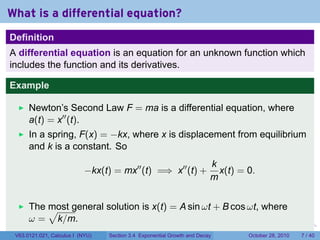
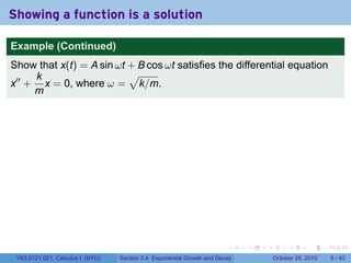
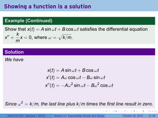
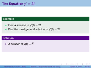
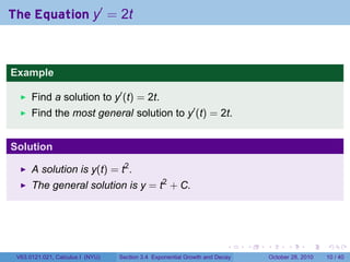
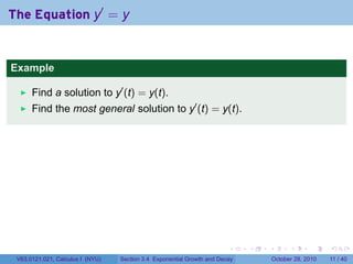
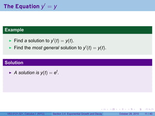
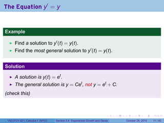

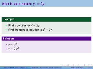
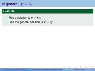
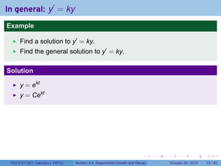
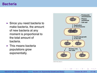
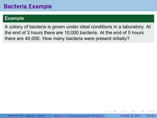

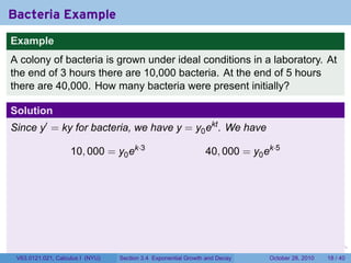
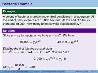
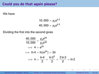
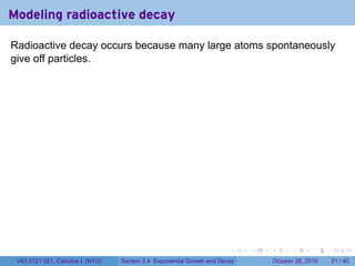
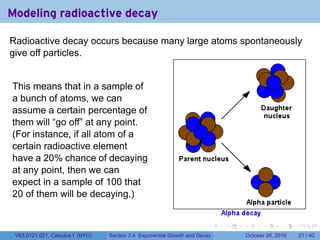
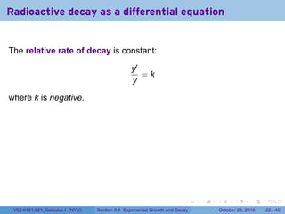
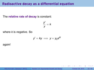
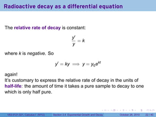
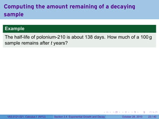
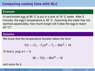
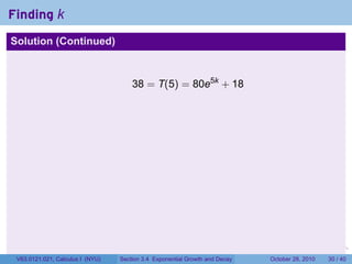
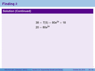
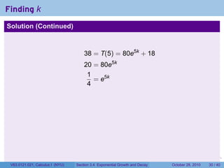
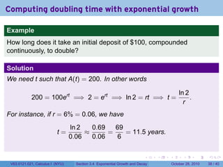

The document presents an overview of exponential growth and decay, specifically through the lens of calculus at NYU. It outlines key concepts such as modeling population growth and radioactive decay using differential equations, with examples and solutions provided for various equations. The material emphasizes the importance and applications of these concepts in real-world scenarios.