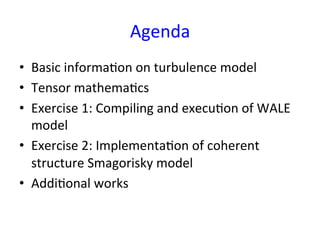
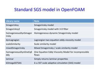
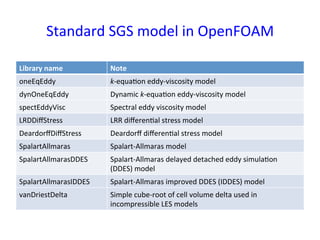
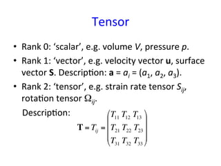
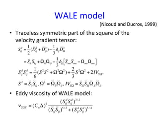
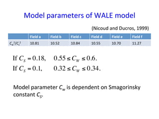
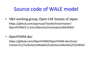
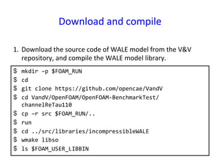
This document provides an in-depth overview of turbulence modeling in OpenFOAM, focusing on the customization of the LES turbulence model and several associated exercises. It covers theoretical aspects of turbulence models, including the Smagorinsky and Wale models, and offers practical instructions for compilation and execution of these models using source codes. Additionally, it discusses tensor mathematics relevant to turbulence modeling and outlines specific tasks for implementing these models in simulations.
![Original
source
codes
for
SGS
model
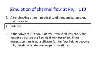
$ src
$ cd
turbulenceModels/incompressible/LES/
$ ls
1. Check
the
original
source
code
for
SGS
model.
2. Glance
the
codes
of
Smagorinsky
model.
$ gedit
Smagorinsky/Smagorinsky.*
3. In
this
exercise,
we
look
the
codes
of
dynamic
models.
$ ls
*[Dd]yn*
4. Compare
the
structures
and
statements
of
the
related
codes
(*.C
and
*.H).](https://image.slidesharecdn.com/lescustomizationen-150615153813-lva1-app6892/85/Customization-of-LES-turbulence-model-in-OpenFOAM-34-320.jpg)