MSc Thesis - Jaguar Land Rover

CRANFIELD UNIVERSITY
School of Aerospace, Transport and Manufacturing
M.Sc. Thesis
Academic Year: 2015-2016
Akshat Srivastava
The Impact of Unsteadiness on Uncertainty in Automotive
Aerodynamics Simulation using OpenFOAM
Supervisor:
Dr. Panagiotis Tsoutsanis
© Cranﬁeld University, 2016.
All rights reserved. No part of this publication may be reproduced
without the written permission of the copyright holder.

Except where acknowledged in the customary manner, the material presen-
ted in this thesis is, to the best of my knowledge, original and has not been
submitted in whole or part for a degree in any university.
________________________
Akshat Srivastava

Abstract
The Detached Eddy Simulation (DES) is performed for flow over sphere. The simula-
tions are carried out based on free-stream Mach number M∞ = 0.2 and sphere diame-
ter D = 1m in sub-critical regime at Re = 10,000. A cartesian grid is generated using
CfMesh in OpenFOAM and computations are performed using PIMPLE Foam solver.
For this Reynolds number at near to the equator of the sphere, flow separates laminarly
and in the separated shear layer the transition to turbulence occur at certain distance.
The frequency spectrum using probes at different locations are described and discussed
in details. The three main instabilities of different frequencies shed from sphere surface
namely, the large-scale vortex shedding at St = fvs D/U = 0.203, the Kelvin Helmholtz
and a frequency lower than the vortex shedding frequency known a low-frequency which
attributes to the shrinkage and enlargement of recirculation bubble. Additionally, turbu-
lence statistics are compared with previous experimental and numerical results available
in literature for sub-critical Reynolds number. Specific consideration is dedicated to com-
puting the mean flow statistics and parameters such as mean angular pressure and skin
friction coefficient, mean lift and drag coefficient, among others, to validate the solver
and turbulence model used.
Keywords: turbulence, sphere flow, OpenFOAM, vortex-sheding, low-frequency, wake
v

Acknowledgements
The work described in this report is the result of my 3 months thesis performed at Cran-
ﬁeld University, UK. Many people contributed their guidance for completion of this thesis
work. I would like to thank everyone who helped me in one way or another and few people
in particular.
First and foremost, I would like to thank Jaguar and Land rover (JLR) for providing me
an opportunity to work in this industrial thesis. My supervisor Dr. Panagiotis Tsoutsanis
has been a great help through his valuable guidance, support and direction. It is my ﬁrst
experience working in turbulence subject, hence, his knowledge and expertise guided me
to understand the project better.
Finally, I would like to thank all the other people for their help at various stages
through the project. I heartily appreciate all your sincere efforts.
vi

Contents
Abstract v
Acknowledgements vi
List of Figures xii
List of Tables xiii
1 Introduction 1
1.1 Background and Motivation . . . . . . . . . . . . . . . . . . . . . . . . 1
1.2 Literature Review . . . . . . . . . . . . . . . . . . . . . . . . . . . . . . 2
1.2.1 Experimental Background . . . . . . . . . . . . . . . . . . . . . 2
1.2.2 Previous Numerical Investigation . . . . . . . . . . . . . . . . . 4
1.3 Thesis Objectives . . . . . . . . . . . . . . . . . . . . . . . . . . . . . . 6
1.4 Outline . . . . . . . . . . . . . . . . . . . . . . . . . . . . . . . . . . . 7
2 Physics and Modelling 8
2.1 Governing Equation . . . . . . . . . . . . . . . . . . . . . . . . . . . . . 8
2.2 Turbulence models and Numerical methods . . . . . . . . . . . . . . . . 9
2.2.1 RANS principle . . . . . . . . . . . . . . . . . . . . . . . . . . . 10
2.2.2 LES principle . . . . . . . . . . . . . . . . . . . . . . . . . . . . 13
2.2.3 Filtered Navier-Stokes equation . . . . . . . . . . . . . . . . . . 15
2.3 Turbulence closure model . . . . . . . . . . . . . . . . . . . . . . . . . . 16
2.4 RANS-LES Hybrid approach . . . . . . . . . . . . . . . . . . . . . . . . 17
2.4.1 Detached Eddy Simulation (DES) . . . . . . . . . . . . . . . . . 18
2.4.2 Delayed Detached Eddy Simulation (DDES) . . . . . . . . . . . 19
2.5 Improved Delayed Detached Eddy Simulation (IDDES) . . . . . . . . . . 20
2.5.1 Modiﬁcation of the Sub-grid length-scale . . . . . . . . . . . . . 21
2.5.2 DDES branch of IDDES . . . . . . . . . . . . . . . . . . . . . . 23
2.5.3 WMLES branch of IDDES . . . . . . . . . . . . . . . . . . . . . 23
vii

Contents
2.5.4 Hybrid branch of DDES and WMLES . . . . . . . . . . . . . . . 25
3 Software and Methodology 27
3.1 OpenFOAM . . . . . . . . . . . . . . . . . . . . . . . . . . . . . . . . . 27
3.1.1 Utilities and Solvers . . . . . . . . . . . . . . . . . . . . . . . . 28
3.1.2 Case structure in OpenFOAM . . . . . . . . . . . . . . . . . . . 29
3.2 OpenFOAM Discretization . . . . . . . . . . . . . . . . . . . . . . . . . 30
3.2.1 Spatial discretization . . . . . . . . . . . . . . . . . . . . . . . . 32
3.2.2 Time discretization . . . . . . . . . . . . . . . . . . . . . . . . . 34
3.2.3 Momentum-Pressure Coupling . . . . . . . . . . . . . . . . . . . 34
3.2.4 Implementation of Turbulence Model . . . . . . . . . . . . . . . 35
3.3 Simulation Overview . . . . . . . . . . . . . . . . . . . . . . . . . . . . 36
3.4 Solvers, Smoothers and Preconditioners . . . . . . . . . . . . . . . . . . 37
4 Computational Methodology 39
4.1 Computational domain . . . . . . . . . . . . . . . . . . . . . . . . . . . 39
4.2 Initial and Boundary conditions . . . . . . . . . . . . . . . . . . . . . . . 40
4.3 Time step selection . . . . . . . . . . . . . . . . . . . . . . . . . . . . . 42
4.4 Mesh Generation . . . . . . . . . . . . . . . . . . . . . . . . . . . . . . 43
4.4.1 Procedure . . . . . . . . . . . . . . . . . . . . . . . . . . . . . . 44
4.4.2 Refinement . . . . . . . . . . . . . . . . . . . . . . . . . . . . . 47
4.5 Mesh dependent study . . . . . . . . . . . . . . . . . . . . . . . . . . . 51
5 Results and Discussions 55
5.1 Frequency spectrum analysis . . . . . . . . . . . . . . . . . . . . . . . . 55
5.2 Instantaneous flow . . . . . . . . . . . . . . . . . . . . . . . . . . . . . 62
5.3 Mean flow parameters . . . . . . . . . . . . . . . . . . . . . . . . . . . . 67
5.4 Mean flow statistics . . . . . . . . . . . . . . . . . . . . . . . . . . . . . 71
6 Conclusion and Future work 78
6.1 Conclusion on thesis . . . . . . . . . . . . . . . . . . . . . . . . . . . . 78
6.2 Recommendations for future work . . . . . . . . . . . . . . . . . . . . . 80
Bibliography 82
Appendices 88
A controlDict 88
B fvSolution 93
viii

Contents
C fvSchemes 97
D meshDict 100
E Mesh comparative study 103
ix

List of Figures
2.1 Energy spectrum of length scales. a) High energy region, b) transfer of
energy region c) dissipation region [36] . . . . . . . . . . . . . . . . . . 13
2.2 Filtering operation for a flow variable [38] . . . . . . . . . . . . . . . . . 15
2.3 Examples of three mesh design during grid refinments [38] . . . . . . . . 19
2.4 Sub-Grid length scale [38] . . . . . . . . . . . . . . . . . . . . . . . . . 22
2.5 Blending function profiles [38] . . . . . . . . . . . . . . . . . . . . . . . 24
3.1 Case Structure of incompressible IDDES simulation . . . . . . . . . . . . 30
3.2 Finite Volume Method . . . . . . . . . . . . . . . . . . . . . . . . . . . 31
3.3 General overview of log file . . . . . . . . . . . . . . . . . . . . . . . . 37
3.4 Schematic overview of OpenFOAM simulation . . . . . . . . . . . . . . 38
4.1 Schematic of computational domain for simulation . . . . . . . . . . . . 40
4.2 ICEM CFD mesh . . . . . . . . . . . . . . . . . . . . . . . . . . . . . . 41
4.3 Velocity magnitude contour for structured mesh generated using cfMesh . 45
4.4 Computational domain geometry . . . . . . . . . . . . . . . . . . . . . . 45
4.5 Patch file example . . . . . . . . . . . . . . . . . . . . . . . . . . . . . . 46
4.6 File format conversion from STL to FMS format using command surfa-
ceToFMS . . . . . . . . . . . . . . . . . . . . . . . . . . . . . . . . . . 46
4.7 Volume refinement using sphere and cone objects . . . . . . . . . . . . . 48
4.8 Patch refinement for sphere . . . . . . . . . . . . . . . . . . . . . . . . . 48
4.9 Prismatic layers using boundaryLayers dictionary . . . . . . . . . . . . . 49
4.10 Velocity contour for mesh validation . . . . . . . . . . . . . . . . . . . . 50
4.11 Pressure contour for mesh validation . . . . . . . . . . . . . . . . . . . . 50
4.12 Y+ contours; (a) Course Mesh, M1 (b) Medium Mesh, M2 (c) Fine Mesh,
M3 . . . . . . . . . . . . . . . . . . . . . . . . . . . . . . . . . . . . . . 52
4.13 Cut plane and Zoom view; (a) Course Mesh, M1 (b) Medium Mesh, M2
(c) Fine Mesh, M3 . . . . . . . . . . . . . . . . . . . . . . . . . . . . . 52
4.14 Time history of Lift and Drag Coefficient plots for entire simulation time
t=9.048, showing transition stage passes after 75D/U time units or 1.1sec. 53
x

List of Figures
4.15 FFT analysis at Probe location-9 showing non-dimensional vortex shed-
ding frequency for (a)M1=0.181 (b)M2=0.211 and (c)M3=0.203 . . . . . 54
5.1 Location of computational probes and lines . . . . . . . . . . . . . . . . 55
5.2 FFT analysis of the streamwise velocity fluctuation at probe P9 (x/D =
2.0, r/D = 0) . . . . . . . . . . . . . . . . . . . . . . . . . . . . . . . . 57
5.3 Time history and FFT analysis at different locations: (a,b) radial velocity
and FFT of it at probe P1, (c,d) radial velocity and FFT of it at probe P2,
(e,f) radial velocity and FFT of it at probe P9, (g,h) radial velocity and
FFT of it at probe P4 . . . . . . . . . . . . . . . . . . . . . . . . . . . . 59
5.4 Energy dissipation in downstream of sphere wake (a) Probe location P9
(x/D = 2.0, r/D = 0), (b) Probe location P4 (x/D = 3.0, r/D = 0.6) . . 60
5.5 (a)Time history of streamwise velocity at probe P9, and (b) time history
of pressure coefficient at P2 . . . . . . . . . . . . . . . . . . . . . . . . . 61
5.6 Cross-correlation between streamwise velocity fluctuation at probe P9
and pressure coefficient at probe P2 . . . . . . . . . . . . . . . . . . . . 62
5.7 Vortex shedding at every quarter time period using Q-iso-surfaces (advan-
cing from (a) to (d)), in X-Y plane . . . . . . . . . . . . . . . . . . . . . 65
5.8 Vortex shedding at every quarter time period using Q-iso-surfaces (advan-
cing from (a) to (d)), in X-Z plane . . . . . . . . . . . . . . . . . . . . . 66
5.9 Instantaneous contours of pressure coefficient, Cp; (a) Coarse mesh, M1;
(b) Medium mesh, M2; and (c) Fine mesh, M3 . . . . . . . . . . . . . . . 68
5.10 Instantaneous contours of non-dimensional skin-friction coefficient,(τ/(ρU2 Re0.5));
(a) Coarse mesh, M1; (b) Medium mesh, M2; and (c) Fine mesh, M3 . . . 69
5.11 Angular distribution of mean pressure coefficient and skin friction coeffi-
cient around sphere; compared with experimental results of Kim & Durbin[14]
at Re = 4200, Bakic[16] at Re = 50000 and DNS results of Seidle et
al.[24] at Re = 5000. . . . . . . . . . . . . . . . . . . . . . . . . . . . . 70
5.12 Streamwise velocity profile along the wake centre line . . . . . . . . . . 71
5.13 Streamwise velocity profile for M1, M2 and M3 at three locations in the
wake, compared with the experimental data of Kim & Durbin at Re=3700 72
5.14 Mean velocity profiles along the wake centre line . . . . . . . . . . . . . 73
5.15 Mean streamwise and radial (cross-stream) velocity profile at different
locations in the wake of sphere . . . . . . . . . . . . . . . . . . . . . . . 75
5.16 Fluctuating mean streamwise and radial (cross-stream) velocity profile at
different locations in the wake of sphere . . . . . . . . . . . . . . . . . . 75
5.17 Contours of normalised mean Reynolds stresses for (a) Coarse mesh, M1;
(b) Medium mesh, M2; and (c) Fine mesh, M3 . . . . . . . . . . . . . . . 76
xi

List of Figures
5.18 Contours of normalised mean shear stress and Turbulent kinetic energy
for (a) Coarse mesh, M1; (b) Medium mesh, M2; and (c) Fine mesh, M3 . 77
E.1 Vortex shedding at same time period for all three mesh using Q-iso-surfaces,
in X-Y plane . . . . . . . . . . . . . . . . . . . . . . . . . . . . . . . . 103
E.2 Instantaneous streamwise velocity contours for; (a) Coarse mesh, M1 (b)
Medium mesh, M2 and (c) Fine mesh, M3 . . . . . . . . . . . . . . . . . 104
E.3 Instantaneous cross-stream velocity contours for; (a) Coarse mesh, M1
(b) Medium mesh, M2 and (c) Fine mesh, M3 . . . . . . . . . . . . . . . 105
E.4 Instantaneous Mach number contours for; (a) Coarse mesh, M1 (b) Me-
dium mesh, M2 and (c) Fine mesh, M3 . . . . . . . . . . . . . . . . . . . 106
xii

List of Tables
2.1 Values of constants in Spalart-Allmaras model . . . . . . . . . . . . . . . 17
3.1 Utilities in OpenFOAM . . . . . . . . . . . . . . . . . . . . . . . . . . . 28
3.2 Incompressible solvers in OpenFOAM . . . . . . . . . . . . . . . . . . . 29
4.1 Initial values for simulation . . . . . . . . . . . . . . . . . . . . . . . . . 42
4.2 Summary of simulation time and DESModelRegions for all three mesh . 43
4.3 M1, M2, M3 representa the coarse, medium and fine mesh while exper-
imental data for vortex shedding Strouhal number and separation angle
from Achenbach [1, 2] and drag coefficient from Schlichting [55] . . . . . 51
5.1 Probes locations used initially for finding the correct positions to captures
the main frequencies associated with the fluctuations . . . . . . . . . . . 56
5.2 Mean flow statistical data, DES (present simulation) results compared
with DNS and LES results at Re=10000 . . . . . . . . . . . . . . . . . . 67
5.3 Mean flow statistics compared with DNS results of Rodriguez et al.[7] at
Re = 3700 and LES results of Constantinescu & Squires[29] at Re = 104 . 74
xiii

Nomenclature
Abbrevations
Cd Drag Coefficient
Cf Skin-friction Coefficient
CFD Computational Fluid Dynamics
CFL Courant Number
Cl Lift Coefficient
Cp Pressure coefficient
CV Control Volume
DDES Delayed Detached Eddy Simulation
DES Detached Eddy Simulation
DNS Direct Numerical Simulation
FFT Fast Fourier Transform
FV Finite Volume
GAMG Geometric-algebraic multi-grid solver
IDDES Improved Delayed Detached Eddy Simulation
LES Large Eddy Simulation
PBiCG Preconditioned Bi-Conjugate Gradient
PCG Preconditioned Conjugate Gradient
PISO Pressure Implicit with Splitting of Operators
xiv

Nomenclature
RANS Reynolds Averaged Navier-Stokes
S-A Spalart-Allmaras turbulence model
SGS Sub-Grid Scale
SIMPLE Semi-Implicit Method for Pressure-Linked Equations
St Strouhal number
URANS Unsteady Reynolds Averaged Navier-Stokes
WMLES Wall Modeled Large Eddy Simulation
Greek Symbols
∆ Filter width m
δ Boundary layer thickness m
ε Energy dissipation rate m2/s3
κ Von Karmann constant −
µ Dynamic viscosity m2/s
ν Kinematic viscosity m2/s
νt Turbulent viscosity m2/s
τw Wall shear stress N/m2
˜ν Modiﬁed turbulent kinematic viscosity m2/s
Roman Symbols
ρ∞ free-stream density kg/m3
P Cell centroid −
R Neighbouring Cell centroid −
˜d DES length m
c Speed of sound m/s
Ck Kolmogorov constant −

Nomenclature
dw Wall distance m
f Frequency 1/s
fb Step function - IDDES −
fe Elevating function - IDDES −
k Wave number 1/s
lhyb Hybrid RANS-LES length scale m
M∞ free-stream Mach Number −
Q Second invariant tensor −
U∞ free-stream velocity m/s
uτ Friction velocity m/s
vivj Velocity components m/s
y+ Distance in wall units −
Mathematical Symbols
¯u ﬁltered velocity m
∇ Nabla operator −
lDES DES model length scale m
q Energy source term −
Re Reynolds number −
t Time s
u Velocity ﬂuctuations m/s
xvi

Chapter 1
Introduction
1.1 Background and Motivation
The flow around bluff bodies such as vehicle aerodynamics, flow around wings at hight
angle of attack, interaction of gust with buildings, heat transfer improvements, among
others are some of the large number of examples which are of great interest for vari-
ous engineering applications. Prediction of flow around such bluff bodies which shows
massive separation, are still remain one of the greatest challenges to the Computational
Fluid Dynamics (CFD). Truth be told, the investigation of turbulent flow past canonical
geometries can be valuable to explore these complex flow structures and additionally to
give valuable data for validation of CFD models (e.g. LES, DES models). In this sense,
the fundamental approach of the present work is to investigate the turbulent flow past a
sphere at sub-critical Reynolds number (laminar boundary layer separation; transition to
turbulence occurs in the separated shear layer). Prediction of flow at supercritical Reyn-
olds number (turbulent boundary layer separation), increments the burden on the model,
essentially through the need to predict the growth of boundary layer and separation, which
is under the control of RANS model in characteristic DES applications. The cost of en-
tire domain LES at supercritical Reynolds number is not a long way from that of Direct
Numerical Simulation due to resolution needed to capture the turbulence structure, inside
the slender attached boundary layer.
The unsteady flow past a sphere at sub-critical Reynolds number has an intricate nature
characterized by the transition form laminar to turbulent flow in the detached shear layer,
the presence of a turbulent wake behind the sphere and unsteady shedding of vortices.
This turbulent flow has been object of numerous experimental and numerical studies
[1, 2, 3, 4], most of studies provided the data of flow visualization, angular distribu-
tion of skin-friction and pressure coefficients over the sphere surface, vortex shedding
frequency and drag coefficient, among others. In the most recent decades Reynolds-
1

1. Introduction
Averaged Navier-Stokes equations (RANS), Large Eddy Simulations (LES) and Direct
Numerical Simulation (DNS) have turned out to be effective tool for giving time-accurate
helpful data about the flow behaviour. However, one of the important requirements of the
simulation of complex turbulent flow is the expensive measure of computational assets
expected to convey them out. That is why, majority of numerical simulations of the flow
over sphere have been carried out in the laminar regime [5, 6]. However, for turbulent re-
gime there are still very few time-accurate calculations carried out [4, 7]. Besides, a large
number of the numerical works reported since now have been performed utilizing differ-
ent turbulent models, including Large Eddy Simulations (LES) [8, 9, 10] and Detached
Eddy Simulations (DES) [11].
While the geometry is straightforward, the flow around the sphere is very complex to
analyse, having a significant number of difficulties that are hard to precisely capture in nu-
merical models. In this work, flow field behaviour are obtained using Detached Eddy Sim-
ulation (DES), a hybrid method which basically reduces to Reynolds-Averaged Navier-
Stokes (RANS) treatment close to the wall and turns into Large Eddy Simulation (LES)in
the region away from solid surfaces, conditionally grid density should be sufficient[12].
DES is a nonzonal method which is computationally feasible for high Reynolds number
flows, yet likewise determines time-dependent, three-dimensional turbulent motions as in
LES. Past simulation results of this strategy have been good, yielding sufficient expecta-
tions over a wide range of flows and likewise demonstrating that the computational cost
has a weak reliance on Reynolds number, like RANS method, yet at same time give more
reasonable description of unsteady effects.
Despite the fact that extensive research available, analysis of mechanism for transition
in shear-layer, behaviour and quantitative estimation of wake structure are still rare. There
is a serious lack of detailed experimental and numerical data for sphere case, such as low
frequency fluctuations, separation angle, recirculation length, force coefficients, among
others, at higher Reynolds numbers. However to the best of our knowledge, there is no
complete study for sphere case which consider the effects of low frequency fluctuations
in wake. While low-frequency fluctuations in the wake of some other bluff bodies have
been examined by few numerical studies.
1.2 Literature Review
1.2.1 Experimental Background
Turbulent flow past the sphere has been the subject of various experimental investigations
[1, 2, 3, 13, 14, 15]. The essential interest for these investigations included visualization of
primary vortical structure in the wake, understanding the mechanism of vortex shedding,
2

1. Introduction
estimation of frequencies present in the wake, mean pressure coefficient around sphere
and streamwise drag. These studies also attempted to understand and explain the mech-
anism through which wake become unstable. As the Reynolds number increases beyond
the Re = 280, experiments demonstrate that the wake starts to shed vortices in a consistent
manner. With the further increment in Reynolds number the shedding process truns out
to be more unpredictable and complex, and, in the long run, the wake structure becomes
chaotic. Since vortex loops diffuse very quickly, the examination of the wake configura-
tion by the method of classical visualization techniques becomes troublesome. As far as
anyone is concerned, except for the recent investigation by Bakic [16] at Re = 5 × 104,
none of the above experimental investigation had provided the data for velocity compon-
ents and Reynolds stresses in the wake which would be necessary for fully validating the
expectations of a time-accurate numerical simulations.
Chomaz et al. [13] recognized the two primary instability modes present in the wake,
when vortex shedding is there. For Re > 280 large-scale vortices shed from the surface of
sphere. The vortex shedding or the first mode is identified to the large-scale shedding in
the wake. At the limit between the recirculation zone and the exterior fluid, this instability
shows itself as a progressive wave movement with alternate fluctuations produced by the
shear. These fluctuations decide the periodic shedding of the vortices that structure behind
the sphere. The recirculation zone is definitely not axisymmetric. Beginning at Re = 800
there is a second high frequency mode (or spiral mode) connected with the small-scale
shear-layer Kelvin-Helmholtz (K-H) instability on the fringe of the recirculation zone.
This unsteadiness is capable for the distortion of large vortex structure and produce the
vortex rings (subsequently vortex tubes), which shed in a quasi-coherent form inside of
the detached shear layers, hence results in a production of small scale vortices, and, in
the long run, transition to turbulence in the wake. The high frequency mode or the spiral
mode instability is present just in an area limited to the wake immediately downstream
of the sphere and in the detached shear layers, where it is more dominating then the
first or vortex shedding mode. These two instability modes can exists together all the
while upto a threshold Reynolds number, however, experiment results shows some about
its value. Although, most of the experiments discussed so far, caught both modes at
Re = 104, results of Kim et al. [14] and Bakic [16] capture both modes up to Re = 105
and Chomaz et al were able to capture both modes at Re = 3 × 104. While Achenbach
[2] failed to detect both modes beyond Re = 6×103 and Sakamoto and Haniu [3] beyond
Re = 1.5×104.
The relationship between frequencies and the structure of wake is the another issue
of great interest. Sakamoto et al.[3] researched this in their experiment using hot wire as
well as flow visualization techniques. Their observe that, laminar hairpin-shaped vortices
begins to shed at Re = 280 to form a completely laminar wake in periodic and regular
3

1. Introduction
fashion. These hairpin vortices are shed regularly from Re = 280 to around 420 with
frequency of same strength and in the same plane, so the the lateral forces coefficient per-
pendicular to shedding plane is zero all times. While from Re = 420to480,they observed
that shedding direction starts oscillating which is conformed by DNS study of Mittal [17].
At the point when Reynolds number surpasses 800, periodically shedding vortex tube now
covers whole near-wake region, and hairpin like vortices which were laminar earlier now
becomes turbulent, however entire vortex sheet is still laminar which is separating from
the sphere. Even now, as compared to the ones at low Reynolds number, the large struc-
ture vortices still appear to keep up a hairpin-shaped form. Correspondingly, some scale
vortex loops formed as small-scale vortex tubes shed into it, and as the move far from
the sphere, interface with the large vortices. Kelvin-Helmholtz instability is subjected to
these smaller vortex tubes which are laminar initially. Baric in his experiment was able
to capture transition of these vortical structures into turbulence as accompany by roll-up
and pairing processes. The vortex sheet begins to undergoes transition from laminar to
turbulence at Re = 3 × 103 and ends around Re = 6 × 103 when it becomes fully turbu-
lent. The experiment of Baric conforms that, change in the wake structure and integral
parameters is very little with the increase in Reynolds number until very close to the crit-
ical Reynolds number or until the drag crisis. That is, at separation the boundary layer
over the sphere is laminar up to Recrit. Due to the complete transition to turbulence in
the detached shear layer, stabilizing effect is generated which happens from Re = 7×103
to Recrit and results in more regular shedding pattern of the large-scale vortices. Con-
versely, with the Reynolds number, the Strouhal number associated with the shear layer
increases strongly since due to the smaller wavelengths the shear layer becomes unstable.
At Re = 104 the value of Strouhal number is in the range of 1.8 − 2.5 and is detectable
generally in the region of detached shear layer. Taneda [15] observe for Reynolds num-
ber in between 104 −105 that oscillating wake in the azimuthal plane, rotates slowly and
irregularly around the axis through center of the flow, oriented parallel to the main flow
direction. Again, even Taneda in his experiment, did not observe any change in wake
structure upto critical Reynolds number
1.2.2 Previous Numerical Investigation
Several time-accurate simulations of laminar flow over sphere using finite-element meth-
ods were accounted among others by Mansoorzadeh et al. [18], Shen and Loc [19],
Kalro and Tezduyar [20] and Aliabadi and Tezduyar [21], while Johnson and Patel [6]
and Shirayama [22] used finite-difference method approaches. Depending on the authors,
generally the onset of vortex shedding was seen in the range of Re = 280 − 400 and the
considered Reynolds number were upto 103. As compared with the experimental data for
Re 275−285, the onset of vortex shedding in these simulations are relatively spread very
4

1. Introduction
large which in turns implies the different level of accuracy of these codes. These codes
contributes in better understanding of vortex structure in the wake ad vortex-shedding
mechanisms.
Tomboulides and collaborators [4, 8] study the transition of near wake to turbulence
by performing laminar, DNS and LES simulations. They correctly captured the onset of
vortex shedding at around Re = 250−285 in their laminar simulation. For LES and DNS
simulations, they limited the maximum Reynolds number of 2×104 and 103 respectively.
To solve the incompressible Navier-Stokes equations the numerical method employed is
a spectral element-Fourier algorithm, while for LES simulation the SGS model utilised
was based on renormalization group theory.The reported value of Strouhal numbers re-
lated to the shedding and spiral modes by Tomboulides and Orszag [4] is very close to
the experimental value measured by Sakamoto and Haniu [3]; the Strouhal number for
shedding was St = 0.2 which is within 10% of the experimental value. Another group,
Kim and Choi [23] used LES for flow over sphere from Re = 3.7 × 103 to 104 to study
the change in the wake structure. These investigators used hybrid discretization (in lam-
inar acceleration region, upwind and central difference elsewhere) and used the immersed
boundary method in cylindrical coordinates to calculate the turbulent flow past sphere.
At low Reynolds number, the quantitative (velocity profile in wake) agreements with the
Experimental data of Kim and Durbin was goodwhile for both Reynolds number the mean
pressure and drag coefficient and shedding frequency were also in range of experimental
results. DNS simulation is performed by another group, Seidl et al. [24] at Reynolds
number of 5,000. They were able to capture the formation of initially laminar vortex tube
successfully in the detached shear layers, and in addition the mechanism of roll-up and
pairing and transition of these vortices. They also able to get correctly the values of drag
coefficient, Strouhal number, etc with their simulation. Schmid [25] performed several
LES simulation using different SGS models (Smagorinsky, dynamic and no model) at
Re = 5 × 104. To precisely capture the initial formation of vortex tube and its transition
to turbulence, they utilizes the local grid refinement in the separated shear layer using
the finite volume method. They observed that the influence of SGS model is somewhat
minor on mean flow quantities. They had compared their data with the experimental
observations of Bakic and overall agreement of mean flow velocity profile and its fluctu-
ations in the near wake region at same Reynolds number was in agreement. While this
was conversely with the RANS simulation of Poon et al. [26], which was done on same
Reynolds number flow and in their agreement was poor for integral quantities as well as
wake characteristics. The main observation for unmatched results is that they predicted
the transition downstream then the experimental observed location which would effect
the prediction of mean drag coefficient value. Since the value of turbulent kinetic en-
ergy is very high in the free stream, it can be possible that these problems caused due
5

1. Introduction
to the set up of RANS or the mesh density in the separated shear layer. Drikakis [27]
investigated the steady RANS simulation at subcritical and supercritical Reynolds num-
ber using artificial compressibility solver using κ − ε model in conjunction at near wall,
while another researcher group Koschel et al. [28] used no turbulence model at all for un-
structured finite-element scheme. The achievement of these simulation results for getting
mean quantities like pressure of drag coefficient around sphere was restricted.
Some of the recent simulation like, Constantinescu and Squires [29] simulate the flow
over sphere at Re = 104 using Large Eddy Simulation (LES) and Detached Eddy Sim-
ulation (DES). They utilises the 0-type grid which is generated by revolving 2D grid in
azimuthal direction and observed that both methods reproduce the main flow characterist-
ics and vortex shedding phenomena successfully. This group then again performed Direct
Eddy Simulation (DES) for flow over sphere at subcritical and supercritical regimes at
two different Reynolds number Re = 104 and Re = 105 [30], able to capture the mean
flow parameters this time which were in good agreement with the experimental results.
As far as DNS results are concerned there is not much data available for time-accurate
instantaneous and statistical flow data because for three-dimensional (3D) simulation and
time-accurate results demands running simulation for much longer time, adding to the
computational resources there are also fine grid for DNS simulation which further put
load on resources. Then recently Lehmkuhl et al. [31] carried out simulation for flow
dynamics of wake behind sphere at Re = 3700 and 10,000, they performed some through
analysis on unstructured grid by rotating it in azimuthal direction, further more they also
consider the low-frequency fluctuation which effect the shrinkage and enlargement of re-
circulation zone. They have concluded that the vortex formation region is related to the
base-suction coefficient Cpb. They are also able to successfully capture all three dominant
instabilities, i.e.large-scale vortex shedding, small-scale Kelvin-Helmholtz instability and
modulation of the recirculation which occur at very low frequency fm, further to their
analysis, they also pointed out that with increase in Reynolds number the length of recir-
culation zone decreases. Their results are in good agreement with experimental results.
1.3 Thesis Objectives
The main task of the thesis is to simulate flow over automotive body taking sphere as
a test case here. Its is known that flow over bluff bodies causes turbulence in the wake
which effects the aerodynamic properties. There are some low-frequency fluctuations in
the wake which is hard to capture and require longer simulation time in order to predict it
accurately.
In previous section we have discussed some of the instabilities associated with the
flow over sphere and effect of low-frequency among them which causes shrinkage and
6

1. Introduction
enlargement of recirculation bubble. Next two chapters described that hybrid RANS-LES
model could be an appropriate approach for such kind of flows. Therefore, following are
the important consideration which discussed in this study throughout:
1. An open source numerical tool which can able to simulate the incompressible, un-
steady turbulent flow.
2. A turbulence model which can able to capture turbulent flow features such as vortex
shedding, among others, and even then it should be computationally less expensive.
3. A good mesh in for open source tool since it is known that tools like OpenFOAM
are highly sensitive to mesh quality.
4. Selection of suitable initial and boundary conditions, accurate discretization schemes
and solver settings.
5. Time period selection in order to capture the the clear footprints of low-frequency
fluctuations.
6. Validation of results for instantaneous and mean flow parameters with previous ex-
perimental and numerical results at comparable Reynolds number.
1.4 Outline
The general outline of thesis is as follow, the first chapter-1 highlights the previous experi-
mental and numerical background of flow over sphere case and provides the overall intro-
duction to the shedding mechanism. Chapter-2 discuss the hybrid numerical method util-
ised in thesis, a detail discussion of DES, DDES and IDDES approach is given. Chapter-3
provides the detail procedure of numerical tool used and set up for the case with some
basic focus on governing equations used in solver. Chapter-4 discuss the computational
domain, mesh procedure with CfMesh and refinements used for generating all the meshes.
Chapter-5 discuss the results and validate the numerical results of thesis with experimental
and numerical results present in literature. The last chapter-6 conclude the research with
some of the recommendations for future work.
7

Chapter 2
Physics and Modelling
2.1 Governing Equation
The objective of this thesis is to simulate the flow around sphere at subcritical Reynolds
number of 10,000 which represent the external flow aerodynamics as a test case. Sine the
flow is at low Mach number M = 0.2 (Incompressible flow) and subjected to Newtonian
fluid properties, hence to describe the fluid dynamics of the flow here, Navier-Stokes
equation can be assumed as a governing equation. There are basically five equations
consists in a Navier-Stokes equation, first one is the continuity ((2.1), represents mass is
conserved), three momentum equations for each direction ((2.2), represents momentum
is conserved) and last one is the energy equation (2.3, represents energy is conserved).
Dρ
Dt
=
∂ρ
∂t
+∇.ρu = 0 (2.1)
ρu
Dt
=
∂ρu
∂t
+∇.(ρuu) = −∇p+∇.(µ∇u)+ f (2.2)
Dρe
Dt
=
∂ρe
∂t
+∇.(ρue) = −∇pu+∇.(µu∇u)−∇q (2.3)
where, D/Dt = ∂/∂t + u∇ is know as Substantial derivative. Whereas ρ, p,e are the
density, pressure and total internal energy. While u represents the velocity magnitude for
all three directions and the symbol ∇ refers to as Nabla operator which is defined as:
8

2. Physics and Modelling
∇ =
∂
∂x
,
∂
∂x
,
∂
∂x
(2.4)
Since the flow is consider as incompressible flow because of low Mach regime, hence
it results in a homogeneous and constant density across whole domain. The assumptions
made here, results a simpler form of Navier-Stokes equation due to the absence of any
external forces such as body forces or gravity. Also, the temperature is considered con-
stant and assumed that it doesn’t have any influence on the flow field dynamics. All of the
assumptions made here reduces the number of unknowns to just four (all three velocity
components and pressure), while the energy equation can be omitted, equation 2.3. Hence
the resulting equations would be:
∇.u = 0 (2.5)
∂u
∂t
+∇.(uu) = −
∇p
ρ
+∇.(ν∇u) (2.6)
2.2 Turbulence models and Numerical methods
The external flow in Automotive engineering is inherently connected to the turbulence. It
is a phenomena which exists in various engineering and industrial applications. Due to its
wide existence, it is one of the most researched topic of CFD so far and hence there are
various ways available by which different turbulent scale which exists in a turbulent flow
can be computed. Among all the techniques available, Direct Eddy Simulation is the one
which provides the most ’exact’ solution of Navier-Stokes equation since it solves all the
scales in turbulence and hence doesn’t require modelling at all. However DNS has some
serious drawbacks:
1. It has a very very high requirement of computational power (e.g. cost of DNS scale
is ∝ Re3), hence it make DNS very costly for daily use or for initial test simulations.
2. Since the number of cell require to carry out DNS simulation is ∝ toRe9/4, hence
large domain size would result in millions of cells for large Reynolds number and
reducing the domain would results some non-physical changes in flow dynamics.
For Automotive applications we need a large far field to damp out any possibility
of wall effect behind the body of interest.
9

Then there is another method which models the smallest scale (kolmogorov scale)
and computes the most important large scales, knows as Large Eddy Simulation (LES).
Whereas the third one and the most used one in industries is the Reynolds Averaged
Navier-Stokes equation (RANS) which model a very wide range of turbulent length scales.
Now days, a hybrid approach is emerged which combines the advantages of RANS and
LES together, this method is used in thesis. Firstly some of the basic principles of RANS
and LES are discussed.
2.2.1 RANS principle
The Navier-Stokes equations 2.5 and 2.6 can be represents in cartesian coordinate system,
xi(i = 1,2,3). Hence the incompressible equations can be written as:
∂uj
∂xj
= 0 (2.7)
Dui
Dt
≡
∂ui
∂t
+uj
∂ui
∂xj
= −
1
ρ
∂ρ
∂xi
+ν
∂ui
∂xj∂xj
(2.8)
where ui is the cartesian components of velocity
In RANS (Reynolds-Averaged Navier-Stokes equation) method, we averaged out all
the unsteadiness in the flow and regarded as a part of turbulence. Hence the flow velocity
is represented as the sum of two terms:
ui(xi,t) = ¯ui(xi)+ui(xi,t), (2.9)
where,
¯ui(xi) = lim
T→∞
1
T
T
0
ui(xi,t)dt (2.10)
Where T represents the averaging interval, it should be large as compared to the typ-
ical time scale of turbulent fluctuations. While ui represents the time averaged value of
fluctuation.
For unsteady flow problems, ensemble averaging is used in place of time averaging.
The ensemble averaging can be explained as variable that can be controlled (boundary
conditions, energy, etc.) for a set of flows who are identical but initial conditions are
generated randomly. This will give flows that differ considerably from one another. Hence
10

an ensemble average is defined as an average over large set of such flows. Can be written
as:
¯ui(xi) =
1
N
N
∑
n=1
uni(xi,t) (2.11)
Where N represents the number of members of the ensemble. For Reynolds averaging
(unsteady flow) we apply the ensemble average approach to the incompressible continuity
equation 2.7, gives
∂ ¯uj
∂xj
= 0 (2.12)
We take the mean of the left hand side of the momentum equation 2.8, since mean of
convective term is not a easy task because of nonlinearity. Hence equation can be written
as:
Dui
Dt
=
∂ ¯ui
∂t
+
∂(uiuj)
∂xj
(2.13)
Using equation 2.9 for non linear term gives:
uiuj = ( ¯ui +ui)( ¯uj +uj) (2.14)
= ¯ui ¯uj +uj ¯ui +ui ¯uj +uiuj
= ¯ui ¯uj +uj ¯ui +ui ¯uj +uiuj
= ¯ui ¯uj +uiuj (2.15)
Since,
uj ¯ui = uj ¯ui = 0 (2.16)
Using equation (2.15) with equation (2.13), we get
Dui
Dt
=
∂ ¯ui
∂t
+ ¯uj
∂ ¯ui
∂xj
+ ¯ui
∂ ¯uj
∂xj
+
∂(uiuj)
∂xj
(2.17)
Using incompressible mean velocity, equation (2.17) simplifies to
11

Dui
Dt
=
∂ ¯ui
∂t
+ ¯uj
∂ ¯ui
∂xj
+
∂(uiuj)
∂xj
(2.18)
Now taking the mean of the other terms in momentum equation results in Reynolds
(RANS) equation.
∂ ¯ui
∂t
+ ¯uj
∂ ¯ui
∂xj
= −
1
ρ
∂ ¯p
∂xi
+ν
∂ ¯ui
∂xj∂xj
−
∂uiuj
∂xj
(2.19)
Equation (2.19) can be written in a simplified form as:
ρ
∂ ¯ui
∂t
+ ¯uj
∂ ¯ui
∂xj
=
∂
∂xj
− ¯pδij + µ
∂ ¯ui
∂xj
+
∂ ¯uj
∂xi
−ρuiuj (2.20)
On the left hand side, the term in square brackets represents the sum of three stresses;
namely, − ¯pδij represents the mean pressure, the second term represents the viscous stress
from the momentum transfer and the last term −ρuiuj, is the fluctuating velocity. This
term is called Reynolds stresses.
The Reynolds stresses are components of symmetric second order tensor, where the
diagonal components represents normal stresses while non-diagonal components repres-
ents shear stresses. Half the trace of the Reynolds stresses give the turbulent kinetic
energy, k, given by:
k =
1
2
ρuiui (2.21)
Since, six more unknowns are introduced because of the six independent elements due
to symmetry of the Reynolds stress tensor hence, in order to close the system, i.e. number
of unknowns equal to the number of equations, we need to model the Reynolds stresses
in one of the ways given in literatures [32, 33]
Turbulence consists of different size eddies, the largest eddies which are highly un-
stable in a flow, break up and hence transfer their energy to smaller eddies which are also
unstable and break up again to transfer their energy to yet smaller eddies. This is know as
energy cascading and continues until the Reynolds number Re(l) ≡ u(l)l/ν is sufficiently
small so that eddy motion is stable and molecular viscosity is effective in dissipating the
kinetic energy [34].
12

2.2.2 LES principle
Smagorinsky [35], gives the idea and basic theory of LES in 1963. The largest scale
eddies, according to theory of Kolmogorov are the eddies which contain most of the
energy and do most of the transportation hence these eddies are one of the most important
one in turbulence and are calculated directly. While the smallest scale eddies can be
easily modelled since they are assumed to behave uniformly. This is the concise basic
principle of Large Eddy Simulation (LES). Generally expressed, this implies the smaller
scales contributes a small amount of the total energy while the larger scale contain the
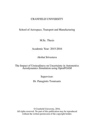
dominant part of the energy. This can be outline by the turbulent energy cascade or energy
spectrum, Figure 2.1. The straight dotted line is also defined in figure which represents
the Kolmogorov’s law and is defined as:
E(k) = Ckε2/3
k−5/3
(2.22)
Where Ck = 1.5, ε is the energy dissipation rate, and k is the wavenumber which is in-
versely proportional to the length scale.
Figure 2.1: Energy spectrum of length scales. a) High energy region, b) transfer of energy
region c) dissipation region [36]
In above Figure 2.1, energy spectrum is divided into three sub-regions:
13

1. Integral length scale: This is the first region and is characterized by largest eddies
which contain the dominate part of energy, denoted by ki.
2. Inertial subrange: The second region in which eddies follows the Kolmogrov’s
law. In this region mostly the transfer of energy from large to small scale is happing
hence it is dominated by transitive scale.
3. Dissipative range: The last and third region contains the smallest scale eddies who’s
behaviour is dominated by the viscosity and energy transfer from the larger scale
eddies.
Like in Reynolds-Averaged Navier-Stokes equations (RANS), 2.2.1; we do some aver-
aging to model the large scale, in Large Eddy Simulation (LES) we apply filtering. The
scale separation is performed using this filtering, which is the locally derived weighted
average of the flow properties over a volume of a fluid. The filter width ∆ is one of the
important feature in filtering operation. ∆ is selected in such a way that, turbulent length
scale larger then it are held in the flow while the Sub-Grid Scales (SGS) or the smaller
scales then ∆ should be modelled. In this way we can write any turbulent flow variable,
like flow velocity, as a sum of large and small scale.
¯u = u−u (2.23)
The resolved larger scale is represented by overbar while smaller scale are represented by
prime. The filter process for large scale is obtain by:
¯u = u(x )G(x,x ;∆)dx (2.24)
Where (x,x ;∆) is know as filter function and it should satisfy the condition:
G(x,x ;∆)dx = 1 (2.25)
The schematic representation of one-dimensional filtering operation for one of the flow
variable is shown in Figure 2.2. The implicit top-hat filter is a standard filter applied in
OpenFOAM (standard filter for Finite Volume methods), which takes an average over a
rectangular region (Some other filters are also exist such as, Gaussian filter or sharp hat
filter [37]). The local and averaged value of ¯u will be equal if we choose fiter width equal
to the grid spacing. It is given by:
G(x,∆) =
1
∆, if | x |≤ ∆
2
0, otherwise
(2.26)
14

Figure 2.2: Filtering operation for a flow variable [38]
2.2.3 Filtered Navier-Stokes equation
Equation of motion is obtained for resolved large scales by applying filter to the incom-
pressible Navier-Stokes equation (2.8), the filtered equations are denoted by overbar:
∂ ¯ui
∂xi
= 0 (2.27)
∂ ¯ui
∂t
+
∂
∂xj
( ¯ui ¯uj) = −
1
ρ
∂ ¯p
∂xi
+
1
ρ
∂τR
ij
∂xj
+ν∇2
¯ui (2.28)
A dependency is caused between unresolved and resolved scales due to the non-linear
convective term of Navier-Stokes equation. The impact of the unresolved scales are con-
solidated in the subgrid-stress tensor, which includes the residual stresses and it is char-
acterized by:
τR
ij = ρ(uiuj − ¯ui ¯uj) (2.29)
15

To define the unresolved scales, an Eddy viscosity model is utilized in LES. Hence stress
tensor becomes:
τR
i j = 2ρνt ¯Sij +
1
3
δijτR
kk (2.30)
Where νt represents turbulent or eddy viscosity. Which gives us:
∂ ¯ui
∂t
+
∂
∂xj
( ¯ui ¯uj) = −
1
ρ
∂ ¯p
∂xi
+2
∂
∂xj
[(ν +νt) ¯Sij] (2.31)
Above equation (2.31) represents the final Filtered Navier-Stokes equation, now the last
step is to give the definition of turbulent-viscosity (νt).
2.3 Turbulence closure model
In the thesis we used Spalart-Allmaras (S-A) turbulence model to determine the turbulent
viscosity (νt). Since S-A model use only one additional equation hence it is relatively
simple. The modified turbulent kinematic viscosity (˜ν) is introduced as the only addi-
tional unknown in the equation. Modified turbulent viscosity is defined by [39]:
νt = ˜ν fv1 (2.32)
where,
fv1 =
χ3
χ3 +c3
v1
χ =
˜ν
ν
Here, ν is the molecular viscosity, cv1 is a contant and ˜ν represents the modified turbulent
viscosity or the working variable, giving the transport equation:
D˜ν
Dt
= cb1
˜S˜ν +
1
cσ
[∇.((ν + ˜ν)∇˜ν)+cb2(∇˜ν)2
]−cw1 fw
˜ν
˜d
2
(2.33)
˜S = ω +
˜ν
κ2 ˜d
fv2 (2.34)
16

fv2 = 1−
χ
1+ χ fv1
(2.35)
Where ω represents magnitude of vorticity while function fw is given by:
fw = g
1+c6
w3
g6 +c6
w3
1/6
(2.36)
g = r +cw2(r6
−r) (2.37)
r =
˜ν
˜Sκ2 ˜d2
(2.38)
The values of constants defined above is tabulated in Table 2.1
Constant Value
cb1 0.135
cb2 0.622
cw2 0.3
cv1 7.1
cσ 2/3
κ 0.41
cw3 2
cw1 cb1/κ2 +(1+cb2)/cσ
Table 2.1: Values of constants in Spalart-Allmaras model
2.4 RANS-LES Hybrid approach
In Hybrid methods, for region near the wall they typically utilises the solution of another
set of model equations. The region where turbulent boundary layer is solved in a zonal
hybrid methods is defined for a region in the vicinity of the wall. While explicit boundary
condition is prescribed for communication to the outer LES region. Where as a smooth
transition between different regions is made in a blended hybrid methods.
Spalart and Allmaras [40] was the first to propose the most widely recognized type
of a hybrid RANS-LES method in 1992, name as, Detached Eddy Simulation (DES). It
combines the advantages of both Reynolds-Averaged Navier-Stokes (RANS) and Large
Eddy Simulation (LES) together, which is the basic thought behind this approach. In
17

a more explanatory way, this hybrid RANS-LES method acts as only RANS mode in
attached boundary layer and transform into LES mode only for detached flow regions.
From the region of unsteady RANS equations to the region where standard LES is solved,
a smooth transition is produced for these blended hybrid methods, while this kind of
switching between RANS and LES relies on the local-grid resolution. Piomelli et al. [41]
had shown that due to the interface treatment resulting form transition layers in DES,
results in decrease of skin friction for these blended approaches. This section give the
overview of the kind of errors in Detached Eddy Simulation (DES) and Delayed Detached
Eddy Simulation (DDES) while dealing with these models and next section 2.5 provide
the solution to overcome these kinds of errors.
2.4.1 Detached Eddy Simulation (DES)
In a classic Detached Eddy Simulation (DES), a limiter combines the standard Spalart-
Allmaras RANS model with its Sub-Grid Scale (SGS), defined by:
lDES = min{dw,CDES∆} (2.39)
where lDES represents the model length scale, dw is the distance to the wall(given by
destructive term of Spalart-Allmaras model), CDES is the derived constant whose value is
0.65 and ∆ is the largest local-grid spacing:
∆ = max{∆x,∆y,∆z} (2.40)
In Detached Eddy Simulation (DES), near the wall (dw < CDES∆) in a attached boundary
layer, a classic S-A RANS is acting, while away from the wall (dw > CDES∆) in a separa-
tion region, a SGS model is acting with a filter CDES∆. Despite the fact that this turbulence
model is most common and utilized for several years, regardless it experiences a few dis-
advantages. Issues emerges when separation region is smaller then the thick boundary
layer in a wall bounded flows. For this situation, often the boundary layer thickness is
larger then the grid spacing parallel to the wall ∆|| or in other words, it grid become fine
enough in for DES length-scales, parallel to the wall such that the LES branch follow
through it in accordance to equation 2.39. Due to this a phenomena is developed which is
called Grid Induced Separation (GIS) [42, 40] according to it, as a consequence of finer
grid, the eddy viscosity reduces below the RANS level but the velocity fluctuations which
are driving the LES content (or resolved Reynolds stresses) have not replaced the modeled
Reynolds Stresses. Hence, these ’missing stresses’ causes the reduction in skin friction.
Figure 2.3 represents the basic grid examples to give the overview of grid importance.
The Figure 2.3a shows the grid in which wall-parallel spacing ∆|| is larger then the
18

(a) Grid spacing larger then the boundary layer
(b) Grid spacing smaller then the boundary
layer,too coarse for LES
(c) Grid spacing to support LES content
Figure 2.3: Examples of three mesh design during grid refinments [38]
boundary layer thickness δ, due to it, in entire the boundary, the DES length-scale is equal
to the RANS type (lDES = dw). Figure 2.3c shows the grid wall-parallel grid spacing less
than to boundary layer thought the domain, traditionally this represents the pure LES type
grid, therefore in most of the boundary layer the SGS model is activated (lDES = CDES∆)
while only in vicinity of wall a RANS model is activated (lDES = dw). In Figure 2.3b, the
wall-parallel grid spacing is not as small as for pure LES grid therefore deep in the bound-
ary layer, a SGS model of DES is originated. It can not able to capture all the velocity
fluctuations since the grid is not fine enough at this point. Besides, without the acquaint-
ance of resolved stresses to re-established the balance the modeled Reynolds stresses and
eddy viscosity will be reduced. In literature this phenomena is called Modeled Stress
Depletion (MSD).
2.4.2 Delayed Detached Eddy Simulation (DDES)
The equivocal grid like Figure 2.3b give rise to the problem like Modeled Stress Depletion
(MSD), hence the method is formulated to avoid these error, called Delayed Detached
Eddy Simulation (DDES) which is just a simple modification of classic Detached Eddy
Simulation (DES) and similar to the shear-stress transport model proposed by Menter et
19

al. [43]. The noticeable feature of DDES is that, to define length-scales it utilises some
blending functions. Even if due to the grid spacing the DES limiter is activated even
though DDES maintains the full RANS mode by detecting the boundary layer which
is dependent on the eddy viscosity and therefore on solution as well. As explained by
the Haase et al. [44], even if blending function showing that point of interest is inside
the boundary layer, it declines to change into LES mode. As an outcome, the transition
between LES-RANS is more abrupt. Hence, the DDES is degigned in such a way that it
wipe out the errors caused by DES to a grid refinement like MSD or GIS.
Menter et al. [43] has given the blending functions F1 and F2 which utilises the
RANS model internal length scale and the wall distance. At the boundary layer, these
function are 1 and at the edge of the boundary layer they reduces rapidly to 0. A para-
meter ”r” is utilized in one equation models (S-A model) since internal length scale is not
present, this parameter is defined as the ratio of model length-scale to the wall distance
and is given for S-A model as:
rd =
νt +ν
max[ Ui,jUi,j,10−10].κ2d2
w
(2.41)
Where Ui,j represents velocity, κ is Von Karman constant and dw represents the wall
distance. ”fd” in log layer is equal to 1 while it reduces to 0 at the edges and is given by:
fd = 1−tanh(8rd)3
(2.42)
It is 0 in whole domain except in LES region (rd << 1) where it reduces to 0. In contrast
to the old definition of DES length-scale given by equation 2.39, a new definition given by
equation 2.43 also consider the modified length scale which depends on turbulent or eddy
viscosity in comparison to to old definition where only grid dependency is considered.
lDES = dw − fdmax(0,dw −CDES∆) (2.43)
Now with the new definition of lDES, based on value of rd even if fd shows point is well
inside the boundary layer, it is possible to reject the LES mode.
2.5 Improved Delayed Detached Eddy Simulation (IDDES)
Another Improved turbulence method is the Improved Delayed Detached Eddy Simula-
tion (IDDES) which overcomes the errors of previous two Classic Detached Eddy Simu-
lation (DES) and Delayed Detached Eddy Simulation (DDES). This method consolidate
the advantages of Delayed Detached Eddy Simulation (DDES) and Wall Modeled Large
20

Eddy Simulation (WMLES), which is the main objective of IDDES model. An alternate
approach is applied to overcome the larger grid resolution requirement which is the basic
demand of classic LES, is known as Wall Modeled LES. Taking example, Schumann [45]
has given a wall-stress model in 1975, has utilized the empirical derived wall functions
along with velocities by considering the first off-wall point in log-layer to calculate an
approximation for wall stresses at the boundary.
Then again, it is likewise conceivable to utilize the DES for these WMLES as was
successfully attempted by Nikitin et al. [46]. The log-layer mismatch (LLM) error is
encountered mostly with WMLES, between the LES and RANS regime. Actually sim-
ulation gives two log layers: outer most layer when distance to the wall is greater then
the local grid size while the RANS model give the inner layer. Due to the mismatch error
LLM, an error of under-prediction of 15 to 20% was noticed in inner and outer layer. Even
though, in comparison to LES, WMLES still save lot of computing time. The IDDES is
developed in such a way that it gives one formula set for both WMLES and DES applic-
ations and also avoid the LLM so that it can be used for complex geometry for different
flows inside a single simulation. The IDDES method can be sub-divided into four parts
to demonstrate how it works [40, 44, 47, 48].
2.5.1 Modification of the Sub-grid length-scale
Common definition of sub-grid scale for classic LES in most of the literature is give as
the cube root of a cell volume, defined as:
∆ = (∆x)2 +(∆y)2 +(∆z)2 (2.44)
Moreover, for the classic DES (section 2.4.1) the decision of the sub-grid length scale is
dependent on maximum of three cell dimensions 2.40. Both definitions give rises to a
problem more precisely with the constants of SGS, which ought to have different con-
stant values for various flow regimes such as free/pure turbulent flow (Decaying Isotropic
Homogeneous Turbulence) or for wall-bounded flows. Hence another definition was set
up to avoid the requirement of different values for different flow regimes. In this new
definition the main idea is to include some wall-distance dependency which gives the a
new definition of sub-grid length scale:
∆ = f(∆x,∆y,∆z,dw) (2.45)
Where dw represents the wall distance hence new formula depends on both, the local cell
size and the wall distance. Therefore three equations can be given by dividing compu-
tational domain into three sub-domains. First one is given by the maximum local-grid
21

spacing just like for classic DES since grid is mostly isotropic away from the wall and
hence it is set as a classic DES case, given by:
∆free = ∆max ≡ max(∆x,∆y,∆z) (2.46)
Second one is given by equation 2.47, the sub-grid length scale in the region close to the
wall should not follow the drop of the wall-normal step. The sub-grid length scale in this
region is defined by wall parallel grid only:
∆wall = const(dw) = f(∆x,∆z) (2.47)
Third and the last one is defined as, region between the away from the wall and the region
close to the wall is assumed to follow as a linear function of dw for the sub-grid length
scale. Furthermore an assumption is made for ∆ that it varies in the range ∆min ≤ ∆ ≤ ∆max.
Combining all the above statements yields one single equation:
∆ = min{max[Cwdw,Cw∆max,∆wn],∆max} (2.48)
Where Cw = 0.15 is a constant based on developed channel flow for LES and ∆wn is the
grid spacing in wall-normal direction. Figure 2.4 is a typical representation of sub-grid
Figure 2.4: Sub-Grid length scale [38]
length scale for a channel flow, where solid line is valid when ∆ ≤ Cwdw. Furthermore as
long as dw ≤ ∆max is valid the value of ∆ remains constant, at this point ∆ =Cw∆max. When
the maximum cell size dimension becomes less then the distance to the wall, dw > ∆max
22

the SGS grows explicitly with ∆ =Cwdw. As the maximum value is reached ∆max, the SGS
remains constant afterwards. The dashed line represents basically a strong wall-normal
stretching. The value of SGS remain constant near to the wall, Cw∆max. Once ∆wn >
Cw∆max, the value of SGS grows explicitly until maximum cell size is reached. It is well
understood that rate is smaller comparatively in the second case since it is unacceptable
for simulations. In contrast to the different SGS models, the IDDES approach utilizes a
very complex method of assessing the grid filter. Other then the wall normal distance,
cell dimensions and height of the cell in wall normal direction have their impact in the
formulation of the grid filter.
2.5.2 DDES branch of IDDES
When inflow conditions are not turbulent then the first branch corresponds to DDES is
activated. The DDES length scale is given by:
lDDES = lRANS − fdmax(0,lRANS −lLES) (2.49)
with lLES = CDESΨ∆ and lRANS = dw The delaying function is given by equation 2.42.
Compared to the classic DES length scale,there is one more factor ψ. The purpose behind
the addition of ψ is on the ground that flow Reynolds number decreases due to decrease
in the sub-grid eddy viscosity with grid refinement. Sooner or later, the DES will miss-
translate and behave like in the vicinity of a wall. As a result, the turbulent viscosity
will drop with respect to the surrounding velocity and length scales through fv and ft
functions.
The functions for Spalart-Allamars model relies on the ratio of the turbulent viscosity
to the molecular viscosity, can be defines according to S-A model: νt/ν or χ ≡ ˜ν/ν.
Moreover, CDES value increased effectively due to the Ψ factor. For Spalart-Allamars
model this shield function Ψ(νt/ν) is defined as:
Ψ2
= min 102
,
1− cb1
cw1κ2 f∗
w
[ft2 +(1− ft2)fv2]
fv1max(10−10,1− ft2
(2.50)
Where constant κ is equal to 0.424. If the sub-grid turbulent viscosity is larger than 10ν,
then the correction become inactive (ψ = 1) and for lower values it becomes stronger.
2.5.3 WMLES branch of IDDES
In WMLES branch, as opposed to the DDES branch, it will be activated only when flow is
turbulent and unsteady and have an adequate grid fineness to resolve eddies in boundary
23

layer. The coupled RANS-LES length scale is utilised to accomplished coupling amongst
them, it is given by:
lWMLES = fB(1+ fe)lRANS +(1− fB)lLES (2.51)
Where fB, blending function is given by:
fB = min{2exp(−9α2
0,1.0} (2.52)
Where α is equal to 0.25− dw
hmax
The blending function fB is determine by the fast switch-
ing mechanism profound inside the boundary layer, between pure RANS and LES modes,
this transition is found in the range of 0.5hmax < dw < hmax wall distance as shown in Fig-
ure 2.5. The main idea behind this function is to provide rapid transition between modes,
for pure RANS mode it is equal to 1 while 0 for LES mode. Another function is deﬁned as
Figure 2.5: Blending function proﬁles [38]
in equation 2.53 is called an "elevating" function. It is formulated to balance the excessive
decrease in modeled Reynolds stress (RANS), which is encountered in the region of inter-
action between RANS and LES interface and thus treats the logarithmic-layer mismatch.
fe = max{(fe1 −1,0}Ψfe2 (2.53)
24

While the function fe1 is defined as:
fe1
dw
hmax
=
2exp(−11.09α2), if α ≥ 0
2exp(−9.0α2), if α < 0
(2.54)
Since α = 0.25, hence clearly fe1 does not depends the solution but only depends on grid.
Therefore this function works for RANS component as an elevating for blended length-
scale given by equation 2.51 for RANS-LES. In transition zone when fB < 1, the function
fe = fB. While function fe2 is given by
fe2 = 1.0−max{ ft, fl} (2.55)
In equation 2.51, for RANS component the intensity of elevating is control by the function
fe2 by utilizing function ft and fl, defined as:
ft = tanh (c2
t rdt)3
(2.56)
fl = tanh (c2
l rdl)10
(2.57)
Here turbulent νt and laminar ν viscosities are represented by subscript t and l respect-
ively, while rdt and rdl are functions which are analogue to function rd and is expressed
by equation 2.41. The parameters rdl and rdt will be around one laminar layer and in log
region of turbulent boundary layer, respectively. Where as ct and cl are constant para-
meters defined for different models. The function fe2 depends on the solution since both
functions ft and fl are analogue to function rd and hence also depends on the solution
while in boundary layer both functions are around one and enforce functions fe1 and fe2
to become 0.
2.5.4 Hybrid branch of DDES and WMLES
For different kind of grid and simulations, the idea is to develop a method which will
automatically switch and select WMLES or DDES mode. A reformulation of length
scale of DDES is necessary since with the current definitions of length scales for DDES
or of WMLES this was not possible. The new definition is given by:
˜lDDES = ˜fdlRANS +(1− ˜fd)lLES (2.58)
25

While modified blending function is given by:
˜fd = max{(1− fdt, fb} (2.59)
Where fdt is given as:
fdt = 1−tanh[(8rdt)3
] (2.60)
The coupled hybrid length scale for both branches DDES and WMLES is given now as:
lhyb = ˜fd(1+ fe)lRANS +(1− ˜fd)lLES (2.61)
It is pointed out that when flow is turbulent, the function fdt is around 1 since rdt << 1.
Furthermore, ˜fd = fB in order to lhyb approaches to lWMLES. While if the flow is laminar,
then the function fe becomes 0 and lhyb approaches to ˜lDDES.
26

Chapter 3
Software and Methodology
This section gives the overview of softer utilized in this thesis and the computational meth-
odology used to achieve the objective. Since there are already much literature available to
use such methodologies hence this chapter provide a more general overview to perform
LES simulations. Moreover, general structure and solver used are also addressed.
3.1 OpenFOAM
OpenFOAM is an object-oriented free open source software which refers to Open Field
Operation and Manipulation. It has basically a collection of libraries, OpenFOAM has
functionality to connect these libraries to solve CFD problems. OpenFOAM is written in
finite volume code, hence equation are discretised in finite volume approach and the solu-
tion is re-written to conform the approach[49]. The main philosophy behind OpenFOAM
is to make it available for every user to modify and re-write any functionality in it (under
General Public License). Under GNU license, OpenFOAM Foundation ensures that it
remain free for all and anyone can contribute to its development, this philosophy leads to
its rapid development and hence it become most widely utilized open source CFD solver.
Even though every year OpenFOAM foundation aims to provide new and improved ver-
sion of OpenFOAM (till now version 3.0.1), still version 2.2 and 2.4 are widely used in
academic and industrial applications. This thesis address OpenFOAM version 2.4, it has
solvers for compressible and incompressible flows to simulate laminar or turbulent flows
(RANS, LES, DES) and heat transfer problems. Another attraction with OpenFOAM is
that it the development team provides range of webinars, consultancy and training support
for industrial users, however for academic enthusiast users it is no cost widely available
open source solver which has a functionality to perform as the user desire.
The key feature of OpenFOAM is that its finite volume code is written in C++ lan-
guage which is widely used among industry and academics. It also has a precompiled
27

3. Software and Methodology
utilities and solvers and also equipped with pre- and post-processing utilities which en-
able users to perform complete simulation free of cost. Hence, the benefits mentioned
above has a potential to find users since it provides both technical and economical bene-
fits.
3.1.1 Utilities and Solvers
OpenFOAM provides many utilities which helps in mesh generation, pre-precessing and
post-processing applications which are available to users in entire work flow. This sec-
tion provides some of the utilities which aids in thesis, since the meshing is done with
another software hence it will be address in later part of the thesis. It is essential to bring
out the fact for new users that OpenFOAM doesn’t provide GUI even though there are
various GUI available for OpenFOAM but mostly are not endorsed by OpenFOAM de-
velopers, the convenient way interact and communicate with it is via written commands
in a terminal window. In terminal the prospective user give the name of solver or utility to
perform tasks and information for a particular utility can be found via entering a commant
’-help’ in a terminal window. Some of the utilities are given in table 3.1.
Utility Task
blockMesh Official block mesher in OpenFOAM
snappyHexMesh Automatic mesh refiner for complex geometries
checkMesh Check mesh quality and report statistics
DESModelRegions Gives the volume percentage over which RANS
and LES is working
forceCoeffs Lift, Drag and Moment coefficients
probes Specify the probe for sampling
probeLocations Show the probes locations
yPlus Report and calculate the y plus for wall patches
wallShearStress Report and calculate shear stress for wall patches
decomposePar Automatically decompose the domain for parallel
processing
reconstructPar Automatically reconstruct the decomposed domain
data
Table 3.1: Utilities in OpenFOAM
The solver utilised in thesis is the incompressible transient solver "pimpleFoam",
which combines the PISO and SIMPLE algorithm together while maintaining the nu-
merical stability even with higher time steps, this solver is used in cojuction with both
28

RANS and LES turbulence models hence for IDDES simulation it would be a perfect
choice. Besides the pimpleFoam solver there are many incompressible as well as com-
pressible solver present in OpenFOAM 2.4, some of the common incompressible solver
based on case structure and set up are explained in table 3.2. For specific problem these
solvers (computer executable) provide find the solution using the algorithms of a particu-
lar solver.
Utility Task
icoFoam A incompressible solver for transient flows that
can be applicable to low Reynolds number applic-
ations like; small MAVs or UAVs, internal fluid
system.
simpleFoam A incompressible solver for steady state flows util-
ises SIMPLE algorithm and can be used for both
laminar and turbulent flow by using RANS in
background.
pisoFoam A incompressible transient solver utilising PISO
algorithm and can be used in conjunction with both
turbulence models RANS and LES.
pimpleFoam A incompressible transient solver utilising both
PISO and SIMPLE algorithms in conjunction.
This solver can be used for larger time steps while
provide the numerical stability during simulation.
It can be used in conjunction with both turbulence
models RANS and LES.
Table 3.2: Incompressible solvers in OpenFOAM
3.1.2 Case structure in OpenFOAM
Domain region (liquid or solid) or the system of equations are specifically connected to
the set up, case structure and design of an OpenFOAM simulation. This sub-section il-
lustrate the case structure and configuration of incompressible IDDES simulation (shown
in Figure 3.1). Inside case folder, there are three sub-directories which require to set up
simulation, in particular 0, constant and system. The user defines the boundary conditions
in 0 directory for simulation which contains one file each for IDDES variables, namely,
pressure, velocity, Sub-grid scale viscosity and S-A turbulent variable. While the simu-
lations requirements which remain same through out the simulation are defined in con-
stant directory, it has sub-directories like polyMesh which contains the mesh information,
29

transportProperties file contains the fluid type, RASProperties contains the S-A closure
model while LESProperties contains the LES model constants and turbulenceProperties
contains the information of type turbulence model (LES). The last and most important
folder which decide stable or diverging simulation is the system folder, it contains atleast
three important files, i.e., controlDict file which contains the information of start and end
time as well as the time step size, fvSchemes file which contains the equation discret-
ization schemes and last one is fvSolution which contains the information of numerical
algorithms to be used for solving system of equations.
Figure 3.1: Case Structure of incompressible IDDES simulation
3.2 OpenFOAM Discretization
As mentioned in previous section 3.1, OpenFOAM utilises Finite volume method for
LES simulations. This section provides the overview of how equations are discretized
in OpenFOAM and which numerical schemes are used in thesis. Even though there are
30

some schemes which provide much better and accurate results but this is beyond the topic
of research right now in this thesis. Some of the default simulation schemes are also used
in this research work.
The basic idea behind the Finite Volume Method (FVM) is to sub-divide or discretize
the domain in space. Since due to the need of solving the equation in time for unsteady
simulation, time-marching method is needed which makes the equations semi-dicretize to
solve the problem.
Figure 3.2: Finite Volume Method
A set of arbitrary shaped Control Volumes (CV’s) are needed for spatial discretization,
and for each control volume a computational point P is defined (example, Figure 3.2).
From the adjacent cell (N) to the current cell (P), a vector d connect the cell centres of
the two, while A represents the normal area vector between the cells for common face.
OpenFOAM defines it variables in this way which results in collocated grid.
As mentioned earlier, for unsteady simulation a temporal discretization is necessary,
or in other words the time interval or time steps (∆t) are required time marching from the
initial conditions.
The task is to discretized the filtered Navier-Stokes equation (2.28) of incompressible,
Newtonian fluid for LES simulation. After integration of control volume and time using
Finite Volume Method (FVM, yields:
V
∇. ¯udV =
∂V
dA. ¯u = 0 (3.1)
31

t+∆t
t
d
dt V
¯udv+
V
∇.( ¯u ¯u)dV −
V
∇.νef f (∇ ¯u+∇ ¯uT
)dv dt =
−
t+∆t
t V
∆ ¯p
ρ
dV dt
(3.2)
The above equation is in second-order due to the presence of the diffusion term which
introduced the second derivative. Since we now that in order to get accurate results, the
order of discretization of equations need to be higher than or equal to the second-order.
Moreover, due to the second order spatial discretization, higher or second-order temporal
discretization would results in much better and time accurate solution. Now by applying
Tylor series to the transport quantities we wold get:
φ(x) = φP +(X −XP).(∇φ)P +ϕ |X −XP|2
(3.3)
∂φ(t)
∂t
=
φ(t +∆t)−φ(t)
∆t
+ϕ(∆t) (3.4)
Sub-sections below provides the discretization for each term in governing equation, ﬁrstly
spatial discretization is discussed followed by temporal.
3.2.1 Spatial discretization
The general discretization integrals utilized for evaluation on control volumes are dis-
cussed here, for more through knowledge one can refer to Jasak [50].
Volume Integral :
Vp
φ(x)dV ≈ φPVP (3.5)
Sur face Integral :
f
φdA = φf Af (3.6)
Divergence Integral :
VP
∇.φdV ≈ ∑
f
Af .φf (3.7)
32

Gradient Integral :
VP
∇φdV ≈ ∑
f
Af φf (3.8)
Convective term discretization
The Divergence integral (equation 3.7) is applied to the convective term for discretization.
It gives:
VP
∇.( ¯uφ)dV = ∑
f
A.( ¯uφ)f = ∑
f
(A.( ¯u)φf = ∑
f
Fφf (3.9)
Where the volume flux through face is given by F = A. ¯Uf . To get values at faces, second
order interpolation is required between the two neighbouring cell values P.
Diffusive term discretization
Discretization for diffusive term is given by:
VP
∇.(ν∇φ)dv = ∑
f
A.(ν∇φ)f = ∑
f
νf A.(∇φ)f (3.10)
By using an interpolation, the scalar term νf can be easily found out. While the term
A.(∇φ)f is highly depended on the mesh, like in equation 3.10, the face gradient φ for
orthogonal mesh can be defined while the vectors A and d are parallel to each other for
such kind of meshes.
A.(∇φ)f = |A|
φN −φP
|d|
(3.11)
Here P and N are neighbour cells. For non-orthogonal meshes, the equation 3.11 is not
valid any more for second order accurate equations. An additional term is introduces
which represents the non-orthogonality.
A.(∇φ)f = |Ad|
φN −φP
|d|
orthogonal
+ A∆. ∇φ
non−orthogonal
(3.12)
The instability can be arise if mesh non-orthogonality is very high since it will create
negative coefficients, which results in reduced accuracy due to limited correction. That is
why a user should always aim for limited non-orthogonality while generating a mesh.
33

3.2.2 Time discretization
Temporal discretization also have various ways for discretizing time just like the spatial
discretization. The transport equations need to be second-order accurate which is the most
critical thing to remember here. One example of the temporal discretization is the Cranck-
Nickolson scheme which is the expensive and undesired in this research but provide most
accurate result, another option is the second order backward differencing scheme.
Backward Differencing
The temporal discretized equation is given by 3.13, which provides second order accuracy
by utilising three time steps to achieve it.
∂φ
∂t
=
3
2φn+1 −φn + 1
2φn−1
∆t
(3.13)
While perfoming the simulation, one try to minimize the turncation errors, still there are
time’s when some errors are introduced due to small variations in face ﬂuxes. These
kind or errors has some serious effects in LES simulation since they cause an additional
diffusion. The main problem arises when these errors go beyound the sub-grid diffusion.
Due to this reason, the cell face Courant number is always try to set below 1 in order
to maintain stability.
CFL =
¯uf .n
|d|
(3.14)
This is the reason behind using very small time step in this research work since it results
in very small temporal diffusion error.
3.2.3 Momentum-Pressure Coupling
Since the thesis consider the PIMPLE algorithm which utilises the merger PISO-SIMPLE
algorithm and hence it uses the idea of SIMPLE mode (relaxation), since we run sev-
eral simulations to obtain the best inner-outer corrector loops (explained in section 3.3)
therefore current simulation doesn’t utilises the relaxation factor idea instead we set the
tolerance of 10−6 by observation of test simulation results which should be enough for
transient simulations.
In PIMPLE algorithm, the momentum equation is calculated ﬁrst after that the pres-
sure equation is calculated and this new pressure is used to re-calculate the momentum
equation which in turns give new pressure by using this new momentum (explained in
schematic overview of OpenFOAM in Figure 3.4).
34

Thi final Navier-Stokes equation is given below: (full derivation is not presented here)
ap ¯up = H −∑
f
A ¯pf (3.15)
∑
f
A
1
ap
f
(∇ ¯p)f = ∑
f
A.
H
ap
f
(3.16)
One can refer to literatures [36] and [50] for full derivation of above equations. Here ap
represents the set of coefficients depending on ¯up. While H vector consist all the terms
like source and convection part except the pressure term. Pressure Implicit with Splitting
of Operators (PISO) algorithm coupled with SIMPLE advantage is preferred for transient
simulations, like in this research work.
3.2.4 Implementation of Turbulence Model
Since we are dealing with Spalart-Allmaras turbulence model in this research work which
was already discussed in section 2.3, it equations follow the classic disctretization method
similar to the one which are discussed so far, hence recalling Spalart-Allmaras equation
once again:
∂ ˜ν
∂t
+∇.(˜ν ¯u)−
1
σ
∇.((ν + ˜ν)+∇˜ν) = cb1
˜S˜ν
production
+
1
σ
cb2(∇˜ν)2
transport
−cw1 fw
˜ν
˜d
2
dissipation
(3.17)
where table 2.1 already represents the constant values and expression for functions. In
order to increase stability of solution, we drive the production term as an explicit function
of ˜νn−1. Given by:
˜νproduction = cb1 |∇× ¯u|+
˜νn−1
κ2 ¯d2
fv2 ˜νn−1
(3.18)
Discretizing transport term as:
˜νtransport =
cb2
σ
∇ñun−1
.∑
f
A˜νf (3.19)
35

Discretizing destructive term as:
˜νdissipation = − cw1 fw
˜νn−1
¯d2
(3.20)
Where n−1 refers to previous time step.
3.3 Simulation Overview
This section emphasis the procedure of solving equation for LES simulation using discret-
ized Navier-Stokes equations which are already discussed. Figure 3.3 gives the general
overview of simulation, where Final Residual is the tolerance. Steps involved in PIMPLE
algorithm are briefly discussed below:
1. For initializing the flow field and to start LES simulation, a RANS solution having
velocity, pressure, eddy viscosity and face fluxes is utilized.
2. The next step is to use previous time step for updating turbulence properties.
3. The momentum and pressure coupling is solved thrice using PIMPLE algorithm
since nOuterCorrectors or nCorrPIMPLE is set to three (external loop correctors,
which are set to 3).
4. The pressure within the PIMPLE loop is corrected twice using PISO algorithm
since nCorrectors or nCorrPISO is set to two (internal loop corrector, which is set
to 2).
5. The velocities are solved using previous flow field equation. A solver that re-
quire a smoother smoothSolver applicable to symmetric matrices is applied. While
symGaussSeidel "Symmetric Gauss-Seidel" is used as a choice of smoother.
6. The pressure equation are solved using PCG "Preconditioned Conjugate Gradient"
solver which is applicable to symmetric matrices. While for a symmetric precon-
ditioner "Diagonal Incomplete-Cholesky" DIC is used to improve computational
efforts of simulation.
7. To sustain the convergence for pressure equation, the non-orthogonal corrector
nNonOrthogonalCorrector which means the pressure field is solved more often
with new calculated value is set to 1. Due to it we can see the pressure equation
36

is solved one more time in PISO loop. It is generally set to either 1 or 0 for LES
simulations.
∇2
p = f(U,∇p) → pnew → ∇2
pnew = f(U,∇pnew) → till nNonOrthogonalCorr is reached
8. The number of outer and inner correctors are chosen in such a way that a certain
tolerance (in this case it is 10−6) on the quantities is achieved. For this research
case the outer corrector 3 and inner corrector 2 with non-orthogonal correctors 1 is
found sufficient to achieve certain tolerance in each iteration.
Figure 3.3: General overview of log file
3.4 Solvers, Smoothers and Preconditioners
Solvers, Smoothers and Preconditioners can save a lot of computational efforts when used
properly. Figure 3.1 represent sub-directory fvSolution under system directory which
contains these settings and conditioners. In Appendix B, applied setting for PIMPLE
algorithm is provided. Generally considered most computational demanding equation is
the pressure equation among others. The Diagonal Incomplete-Cholesky (DIC) was selec-
ted as a preconditioner for pressure equation. According to CFDdirect [51], Geometric-
algebric multi-grid solver (GAMC) would provide much accurate solution and increase
the speed by corsen/refine mesh in stages but during this research work it is found out
that DIC is give more accurate results while GAMC is diverging (reason behind this is
37

Figure 3.4: Schematic overview of OpenFOAM simulation
beyond the scope of this thesis). Moreover it is realised that DIC speed up the solution
and the tolerance limit is achieved in much earlier than GAMC. The Preconditioner Con-
jugate Gradient (PCG) solver is utilized for solving pressure equation. The other terms
are solved using smoothSolver in conjunction with Symmetric Gauss-Seidel (symGauss-
Seidel) as a smoother for symmetric matrices.
38

Chapter 4
Computational Methodology
In previous section we have presented the physics and modelling approach (chapter 2)
used in this thesis which is very small in comparison to the functionality of DES solution
method; fortunately this part is widely explained in various literatures, text books and
publications, hence only the important portion of DES simulation needed (e.g., filtered
Navier-Stokes equations, momentum-pressure coupling and solver used for resultant matrices)
in thesis is presented in previous sections. However this section focus entirely on simula-
tion set-up by firstly introduction of domain selection (including boundary and initial con-
ditions) then time-step selection followed by mesh generation strategy and finally mesh
dependent study.
4.1 Computational domain
The unsteady simulations were performed in OpenFOAM with a sphere diameter D = 1,
whose centre is located at coordinate (0, 0, 0). The computational domain (Figure 4.1)
extends 4.5 diameters in upstream direction as well as in radial outward direction from the
centre of sphere which corresponds to a blockage (area) ratio of approximately 1.2%. The
blockage ratio here is defined as the ratio of sphere frontal (Asphere = 0.785398163) area to
the test section area (Adomain = 63.62). This is proportional to the sphere is hanging inside
the circular pipe with a diameter of D = 9D (here D always represent the diameter of
sphere). Here, the rate of decay of perturbation away from the body determines the extent
of the upstream and radial computational domain. Since it is well known [52] that rate of
decay of perturbation due to the presence of sphere is 1/r3, here r represents the distance
from centre of the sphere. For two-dimensional bluff bodies (i.e. cylinder) the rate of
decay of perturbations is 1/r2, for three-dimensional sphere case this factor is r times
smaller than the corresponding one. Accordingly, the velocity at x = −4.5 is just 0.1%
different form the initial velocity or the free-stream velocity, as per potential hypothesis.
39

4. Computational Methodology
The same contention additionally holds in the radial direction. Moreover, the blockage
factor of the order of 1% are viewed as insignificant when performing simulations or
experiments as already mentioned in few literatures [2, 14]. While computational domain
in downstream direction extends 25 diameter form the centre of sphere. As reported by
Tomboulides and Orszag [4], simulation by performing domain length of 20 diameter in
downstream direction (with same outflow boundary condition) didn’t have any effect in
upstream direction. Still 25D is chosen due to the reason to have atleast 3 to 4 vortical
structures shedding behind the sphere within the domain, it will increase the grid elements
drastically which indeed increase the computational efforts.
Figure 4.1: Schematic of computational domain for simulation
Some mesh were generated with ICEM CFD during initial investigation represented
in Figure 4.2 with more then 1 million cells for both structured and unstructured mesh but
the simulation diverges every time after converting mesh in OpenFOAM format by using
fluent3DMeshToFoam. It is observe that after conversion the domain size increased in all
three direction which can lead to the divergence due to no element present in the increased
length. Further investigation is beyound the scope of current thesis work (remember that
OpenFOAM is an open source code which can have bugs moreover the version used for
this research is 2.4 which is older then the 2016 version 3.0.1). Further details about mesh
is presented in section 4.4.
4.2 Initial and Boundary conditions
The boundary conditions in OpenFOAM are provided in files for initial velocity, pres-
sure and turbulent fields in 0 directory (Figure 3.1). Four patches are generated during
meshing procedure namely; sphere patch, inlet patch, outlet patch and sides (represents
the radial side of the computational domain). Numerous boundary conditions are imple-
ment on final set-up mesh according to simulations and experiments performed earlier,
since OpenFOAM uses different names for defining boundary conditions and due to lack
40

(a) Structure mesh with 1.4 million elements
(b) Unstructured mesh with 1.8 million elements
Figure 4.2: ICEM CFD mesh
of detailed documentation on it, the best and the most suitable boundary conditions are
implemented. They are described in detailed below:
1. Sphere patch: The velocity field is set as fixedValue with value of (0,0,0) which
as the name implies, the velocity over sphere patch is kept fixed at 0 m/s in all
directions. The pressure field is set as zerogradient, which represents the normal
gradient of pressure is zero or Neumann boundary condition. while fixedValue of
0 for turbulent fields or Dirichlet boundary condition.
2. Inlet patch: The Dirichlet boundary condition or fixedValue with a uniform value of
free-stream in x-direction onlyU∞ = (68.058,0,0)m/s is specified. The free-stream
velocity is calculated by using the Mach number of M∞ = 0.2, while dynamic and
kinematic viscosity is calculated by using the Reynolds number formula (equation
4.1), taking free-stream conditions for density (ρ∞ = 1.225kg/m3), pressure p∞ =
101325 pascal, Reynolds number Re∞ = 10,000 and diameter of sphere D = 1m.
Re∞ =
ρ∞U∞D
µ∞
(4.1)
While for initializing pressure field the Neumann type boundary condition is pre-
41

scribed hence zeroGradient is used. Furthermore, turbulent field is calculated using
turbulent intensity of 0.1% which gives the value 0.071444734, a fixedValue is set
using this.
3. Outlet patch: Neumann and Dirichlet boundary condition for velocity and pressure
field respectively, is prescribed in literature [53]. While in OpenFOAM is found that
Neumann type boundary condition for both fields (pressure and velocity) generates
numerically induced oscillations which can easily be avoided by using inletOutlet
boundary condition for velocity and turbulent field (using same values as for inlet
patch). Hence for a daring experiment this boundary condition is used and found
suitable in current research work, while the pressure field is set as fixedValue with
a value of 0 .
4. Sides patch: It represents the cylindrical domain around the sphere at it is set as
symmetry boundary condition for every field which is according to OpenFOAM
guide represents the slip wall for non-planer patches.
Initial Condition Value
Re∞ 10,000
M∞ 0.2
ρ∞ 1.225kg/m3
p∞ 101325 pascal
µ∞ 8.336×10−3 kg/ms
ν∞ 6.805×10−3 m2/s
nuTilda 0.071444734
D 1m
Table 4.1: Initial values for simulation
4.3 Time step selection
Since this research work used PIMPLE algorithm whose main attraction is stability of
simulation for higher time steps, which can be used to advance in time much faster for
unsteady simulation without compromising the stability of solution but some important
physics can be skip if we use higher time step. Considering the total time required for
running the simulation it would be expected to use higher time steps but in this thesis we
are using much smaller time step to capture the effect of low-frequency fluctuation which
is the main task of thesis. Hence a time step is selected using the convection time which
42

50 times less then it. The convection time is given by time required by the flow to pass
the sphere which is equal to tconvection = D/U∞, calculated as 0.01469. Therefore the time
step selected to carry out simulation is 0.00029, ∆t = 0.00029. Moreover the maximum
Courant Number, CFL is set to 0.5 for whole simulation, if the mean Courant number
value exceed 0.5 any time in simulation, the OpenFOAM reports divergence.
Considering the low frequency fluctuation, the time required to run entire simula-
tion should be long enough to capture such low frequencies (more explanation is re-
fchap:results), hence the current simulations are run for 9.048 seconds (see A) which
corresponds to 120 vortex shedding cycles. According to the knowledge of literatures,
this is the longest simulation for flow over sphere at this Reynolds number). For calcu-
lating the vortex shedding, the experimental value of vortex shedding Strouhal number
fvs = 0.195 is used, which gives the frequency of one vortex shedding equals to 13.2713
therefore, corresponding time for one vortex shedding is equal to 0.07535. Using these
calculations it is found out that for one vortex shedding almost 260 time steps are required
which should allow enough time to capture the low-frequency content accurately.
Mesh Number of CPUs Clock time RANS volume% LES volume%
Coarse mesh, M1 32 34 : 47 : 30 ∼ 1.4Days 37.2 62.8
Medium mesh, M2 32 121 : 04 : 00 ∼ 5Days 30.7 69.3
Fine mesh, M3 32 195 : 13 : 01 ∼ 8Days 35.1 64.9
Table 4.2: Summary of simulation time and DESModelRegions for all three mesh
4.4 Mesh Generation
The most challenging part faced during this process is the post-processing, since it not
only require a complete understanding of how OpenFOAM work but also a requires a
solid understanding of flow physics (which is already discussed in 1) work for flow over
sphere case. Therefore the most crucial part of pre-processing is to generate a suitable
mesh which represents the flow physics as close as to the nature. Since a mesh generation
is a time consuming process for complex geometries even with commercial software’s
like ICEM CFD. Some initial meshes were generated using this software package which
generate very good results in Ansys FLUENT but diverges in OpenFOAM after convert-
ing mesh in it’s format. The potential reason behind it is already mentioned in section 4.1.
Hence ICEM meshes are neglected for current research work.
OpenFOAM has its own mesher snappyHexMesh which is considered very powerful
meshing tool among OpenFOAM users. Even though it generates high quality mesh
automatically, still it is not very popular among community due to two reasons, firstly
43

it requires significant amount of RAM memory for implementation and secondly, from
usability viewpoint it is consider very cumbersome for generating inflation layers for high
quality boundary layer grids. Therefore another open source software is consider in this
thesis work which is explained in next section.
4.4.1 Procedure
Due to the problem faced with commercial meshing package, ICEM CFD and due to the
cumbersome nature of OpenFOAM own mesher snappyHexMesh, another open source
software cfMesh is used to generate grid for simulations,it is a mesher for OpenFOAM
provided by Creative Field company. It is a cross-platform library for automatic mesh
generation that is built on top of OpenFOAM and it is compatible with all versions of
OpenFOAM [54].
The Cartesian Mesh is generated using cfMesh, which offers structured mesh as well
as Unstructured Tetrahedral mesh, since Tetrahedral meshes are well-known to not be
optimal for OpenFOAM simulations among users (this statement wasn’t investigated due
to time constrain). Hence a premilary test with Structured as well as Cartesian mesh was
investigated to make the decision for final type of mesh to be run. Since purely Structured
mesh are better, at the condition that cells have a low skewness and/or are aligned with the
flow. While, Cartesian meshes ensures an optimized mesh quality (zero skewness, aspect
ratio equalling one) in the quasi-totality of the domain.
Structured mesh are known to converge better than tetrahedral meshes. It was shown
that OpenFOAM could give bad results when cells are skewed or not well aligned with the
mesh. The best illustration in our case is that the potentialFoam solver, used to initialized
the velocity field, failed to give physical results on a Structured mesh, when it worked fine
on the Cartesian mesh. The main problem to create a high quality structured mesh in our
case is the presence of the sphere, which prevent cells to be aligned with the flow close
to it. Here, an illustration of this after few iterations on the structured mesh Figure 4.3a.
For all these reasons, Cartesian mesh type is better than structured in our case. The
Cartesian mesh generated using cfMesh generated a 3D mesh which containd mostly
hexahedral elements while in transition region, polyhedral elements are present between
the elements of different sizes. The procedure is detailed below, it worth mentioning here
that Carterian mesh generated, introduced automatically one boundary layer which can
be refined further.
1. Geometry: The tool used to prepare the domain’s geometry (Figure 4.1) was Sa-
lome, which provides a CAD module.
2. Patch Creation: Using Salome all patches were created separately namely; sphere,
inlet, outlet and sides. Figure 4.4 shows the patch names.
44

(a) Global view
(b) Zoomed view
Figure 4.3: Velocity magnitude contour for structured mesh generated using cfMesh
Figure 4.4: Computational domain geometry
45

3. STL file preparation: Each patch was then exported in STL format. The name of
the patch was manually added into each STL file (Figure 4.5 shows the example
of sphere patch file). Finally, all STL files were concatenated (copy-pasted) into a
single one.
Figure 4.5: Patch file example
4. File conversion: The STL input file was converted into FMS format using command
surfaceToFMS, which is recommended in the cfMesh documentation and allows
the user to define OpenFOAM patch types (like patch, wall, symmetry, empty, etc.)
before meshing instead of modifying them in the constant/polyMesh/boundary file
after each mesh generation. Figure 4.6 shows the heading of the FMS file which
was used:
Figure 4.6: File format conversion from STL to FMS format using command surfa-
ceToFMS
5. meshDict file: Finally two mandatory field are edited in meshDict file (see, Ap-
pendix D) to start the meshing process using cfMesh:
46

MSc Thesis - Jaguar Land Rover

MSc Thesis - Jaguar Land Rover

Recommended

Recommended

More Related Content

What's hot

What's hot (20)

Viewers also liked

Viewers also liked (20)

Similar to MSc Thesis - Jaguar Land Rover

Similar to MSc Thesis - Jaguar Land Rover (20)

Recently uploaded

Recently uploaded (20)

MSc Thesis - Jaguar Land Rover