Download as PDF, PPTX

![12
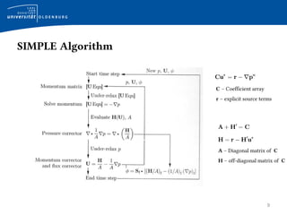
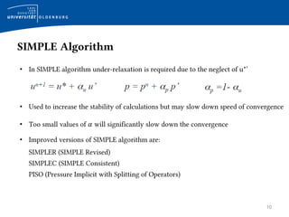
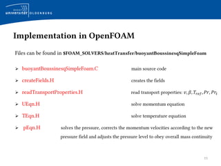
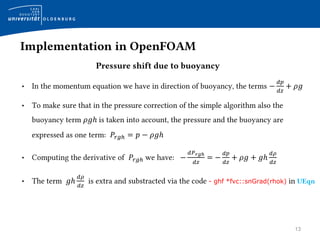
Implementation in OpenFOAM
buoyantBoussinesqSimpleFoam.C
#include "fvCFD.H„ standard file for finite volume method
#include "singlePhaseTransportModel.H„ simple single-phase transport model based on viscosity-Model
#include "RASModel.H„ namespace for incompressible RAS turbulence models
#include "fvIOoptionList.H„ class for external objects or constraints on the case
#include "simpleControl.H„ checks for the simple loop
// * * * * * * * * * * * * * * * * * * * * * * * * * * * * * * * * * * * * * //
int main(int argc, char *argv[])
{
#include "setRootCase.H„ checks folder structure of the case
#include "createTime.H„ checks runtime according to the controlDict and initiates time variables
#include "createMesh.H„ defines mesh in the domain
#include "readGravitationalAcceleration.H„ reads value for g
#include "createFields.H„ creates the fields: T, U, 𝑃𝑟𝑔ℎ, rhok, kappat, gh, turbulence(k, ɛ, nut)
#include "createFvOptions.H„ creates related constraints according to fvOptions
#include "initContinuityErrs.H„ declare and initialise the cumulative continuity error](https://image.slidesharecdn.com/943e2705-4674-453e-af4e-d008ee3bd2a9-160210132604/85/buoyantBousinessqSimpleFoam-12-320.jpg)
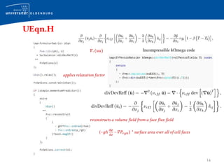
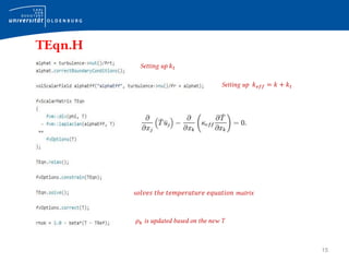
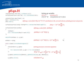
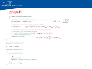
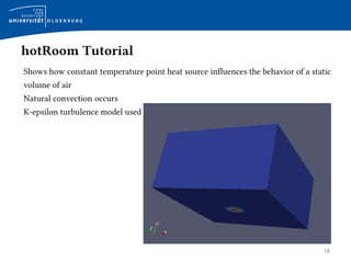
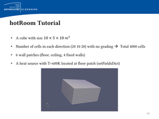
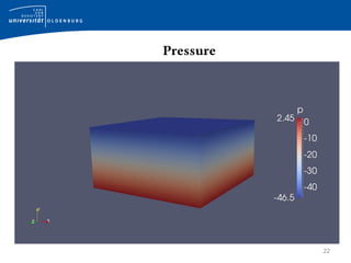
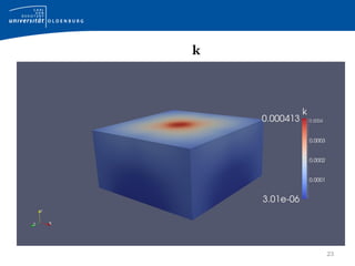


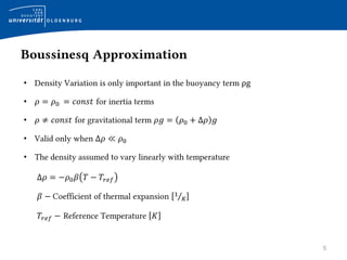
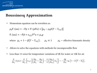
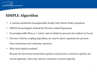
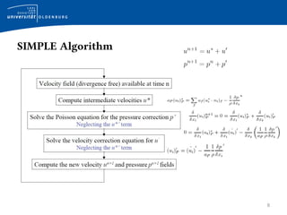
This document provides an introduction to the buoyantBoussinesqSimpleFoam solver in OpenFOAM. It discusses the governing equations including the Boussinesq approximation and SIMPLE algorithm. It then describes the implementation in OpenFOAM, covering the files used, how the pressure, velocity, and temperature equations are solved. Finally, it summarizes the hotRoom tutorial case used to demonstrate natural convection in a room with a heat source.