Downloaded 35 times

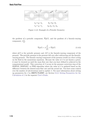
![Basic Fluid Flow
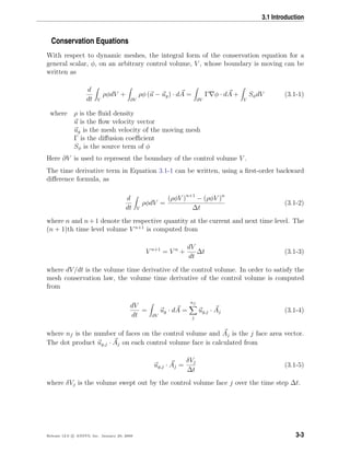
Momentum Conservation Equations
Conservation of momentum in an inertial (non-accelerating) reference frame is described
by [17]
∂
∂t
(ρv) + · (ρvv) = − p + · (τ) + ρg + F (1.2-3)
where p is the static pressure, τ is the stress tensor (described below), and ρg and F are
the gravitational body force and external body forces (e.g., that arise from interaction
with the dispersed phase), respectively. F also contains other model-dependent source
terms such as porous-media and user-defined sources.
The stress tensor τ is given by
τ = µ ( v + v T
) −
2
3
· vI (1.2-4)
where µ is the molecular viscosity, I is the unit tensor, and the second term on the right
hand side is the effect of volume dilation.
For 2D axisymmetric geometries, the axial and radial momentum conservation equations
are given by
∂
∂t
(ρvx) +
1
r
∂
∂x
(rρvxvx) +
1
r
∂
∂r
(rρvrvx) = −
∂p
∂x
+
1
r
∂
∂x
rµ 2
∂vx
∂x
−
2
3
( · v)
+
1
r
∂
∂r
rµ
∂vx
∂r
+
∂vr
∂x
+ Fx
(1.2-5)
and
∂
∂t
(ρvr) +
1
r
∂
∂x
(rρvxvr) +
1
r
∂
∂r
(rρvrvr) = −
∂p
∂r
+
1
r
∂
∂x
rµ
∂vr
∂x
+
∂vx
∂r
+
1
r
∂
∂r
rµ 2
∂vr
∂r
−
2
3
( · v) − 2µ
vr
r2
+
2
3
µ
r
( · v) + ρ
v2
z
r
+ Fr (1.2-6)
where
· v =
∂vx
∂x
+
∂vr
∂r
+
vr
r
(1.2-7)
and vz is the swirl velocity. (See Section 1.5: Swirling and Rotating Flows for information
about modeling axisymmetric swirl.)
1-4 Release 12.0 c ANSYS, Inc. January 29, 2009](https://image.slidesharecdn.com/flth-130501182911-phpapp02/85/Flth-28-320.jpg)
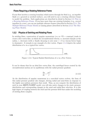

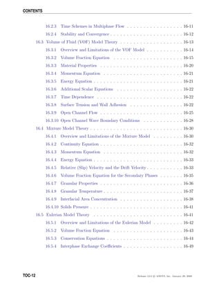
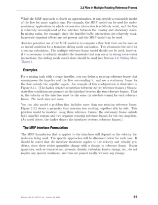
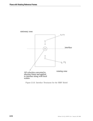
![Flows with Rotating Reference Frames
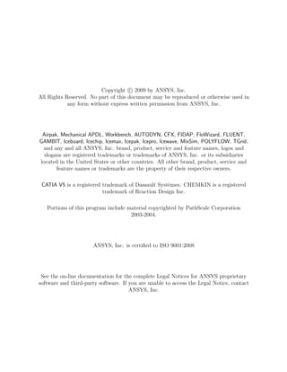
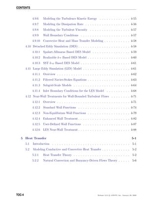
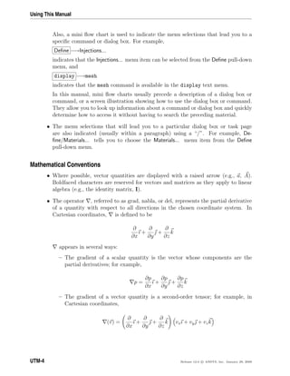
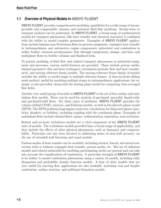
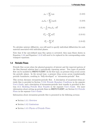
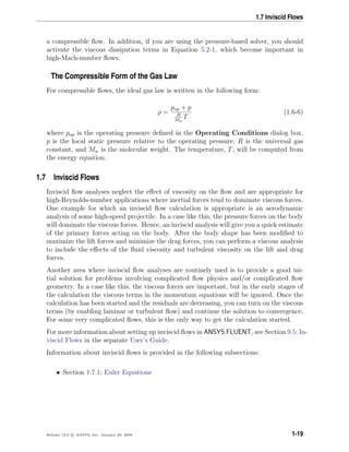
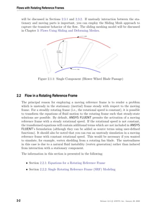
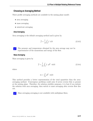
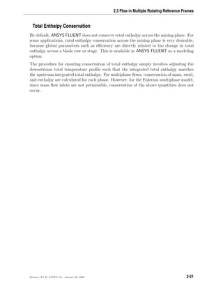
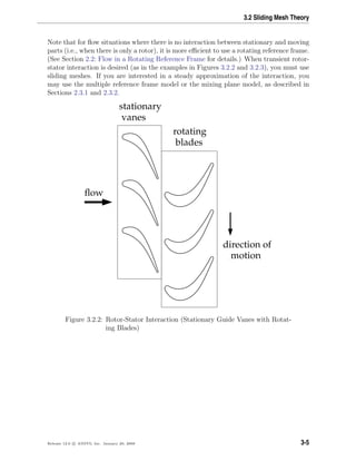
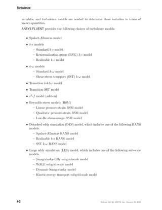
Figure 2.2.1: Stationary and Rotating Reference Frames
In the above, vr is the relative velocity (the velocity viewed from the rotating frame), v
is the absolute velocity (the velocity viewed from the stationary frame), and ur is the
“whirl” velocity (the velocity due to the moving frame).
When the equations of motion are solved in the rotating reference frame, the accel-
eration of the fluid is augmented by additional terms that appear in the momentum
equations [17]. Moreover, the equations can be formulated in two different ways:
• Expressing the momentum equations using the relative velocities as dependent vari-
ables (known as the relative velocity formulation).
• Expressing the momentum equations using the absolute velocities as dependent
variables in the momentum equations (known as the absolute velocity formulation).
The exact forms of the governing equations for these two formulations will be provided
in the sections below. It can be noted here that ANSYS FLUENT’s pressure-based solvers
provide the option to use either of these two formulations, whereas the density-based
solvers always use the absolute velocity formulation. For more information about the
advantages of each velocity formulation, see Section 10.7.1: Choosing the Relative or
Absolute Velocity Formulation (in the separate User’s Guide).
2-4 Release 12.0 c ANSYS, Inc. January 29, 2009](https://image.slidesharecdn.com/flth-130501182911-phpapp02/85/Flth-50-320.jpg)

![Flows with Rotating Reference Frames
2.3 Flow in Multiple Rotating Reference Frames
Many problems involve multiple moving parts or contain stationary surfaces which are
not surfaces of revolution (and therefore cannot be used with the Single Reference Frame
modeling approach). For these problems, you must break up the model into multiple
fluid/solid cell zones, with interface boundaries separating the zones. Zones which contain
the moving components can then be solved using the moving reference frame equations
(Section 2.2.1: Equations for a Rotating Reference Frame), whereas stationary zones can
be solved with the stationary frame equations. The manner in which the equations are
treated at the interface lead to two approaches which are supported in ANSYS FLUENT:
• Multiple Rotating Reference Frames
– Multiple Reference Frame model (MRF) (see Section 2.3.1: The Multiple Ref-
erence Frame Model)
– Mixing Plane Model (MPM) (see Section 2.3.2: The Mixing Plane Model)
• Sliding Mesh Model (SMM)
Both the MRF and mixing plane approaches are steady-state approximations, and differ
primarily in the manner in which conditions at the interfaces are treated. These ap-
proaches will be discussed in the sections below. The sliding mesh model approach is,
on the other hand, inherently unsteady due to the motion of the mesh with time. This
approach is discussed in Chapter 3: Flows Using Sliding and Deforming Meshes.
2.3.1 The Multiple Reference Frame Model
Overview
The MRF model [209] is, perhaps, the simplest of the two approaches for multiple zones.
It is a steady-state approximation in which individual cell zones can be assigned different
rotational and/or translational speeds. The flow in each moving cell zone is solved using
the moving reference frame equations (see Section 2.2: Flow in a Rotating Reference
Frame). If the zone is stationary (ω = 0), the equations reduce to their stationary forms.
At the interfaces between cell zones, a local reference frame transformation is performed
to enable flow variables in one zone to be used to calculate fluxes at the boundary of
the adjacent zone. The MRF interface formulation will be discussed in more detail in
Section 2.3.1: The MRF Interface Formulation.
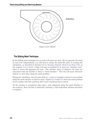
It should be noted that the MRF approach does not account for the relative motion of
a moving zone with respect to adjacent zones (which may be moving or stationary); the
mesh remains fixed for the computation. This is analogous to freezing the motion of the
moving part in a specific position and observing the instantaneous flowfield with the rotor
in that position. Hence, the MRF is often referred to as the “frozen rotor approach.”
2-8 Release 12.0 c ANSYS, Inc. January 29, 2009](https://image.slidesharecdn.com/flth-130501182911-phpapp02/85/Flth-54-320.jpg)

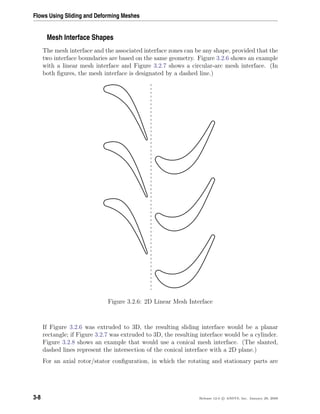
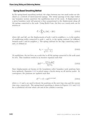
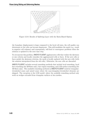
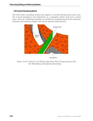
![Flows Using Sliding and Deforming Meshes
In the case of the sliding mesh, the motion of moving zones is tracked relative to the
stationary frame. Therefore, no moving reference frames are attached to the computa-
tional domain, simplifying the flux transfers across the interfaces. In the sliding mesh
formulation, the control volume remains constant, therefore from Equation 3.1-3, dV
dt
= 0
and V n+1
= V n
. Equation 3.1-2 can now be expressed as follows:
d
dt V
ρφdV =
[(ρφ)n+1
− (ρφ)n
]V
∆t
(3.1-6)
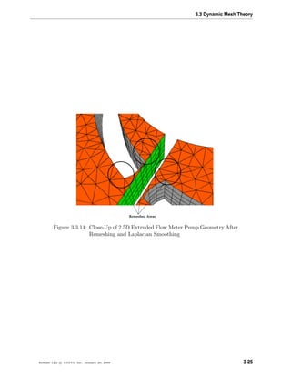
3.2 Sliding Mesh Theory
When a time-accurate solution for rotor-stator interaction (rather than a time-averaged
solution) is desired, you must use the sliding mesh model to compute the unsteady flow
field. As mentioned in Section 2.1: Introduction, the sliding mesh model is the most
accurate method for simulating flows in multiple moving reference frames, but also the
most computationally demanding.
Most often, the unsteady solution that is sought in a sliding mesh simulation is time-
periodic. That is, the unsteady solution repeats with a period related to the speeds of the
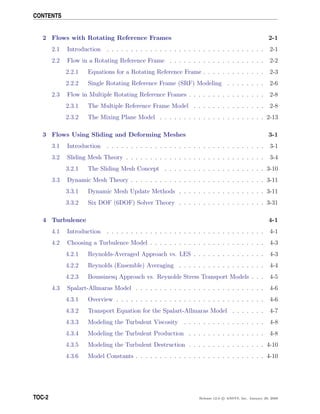
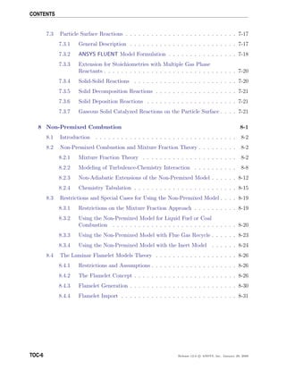
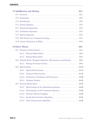
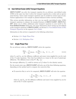
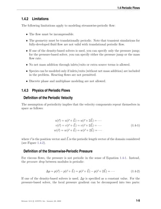
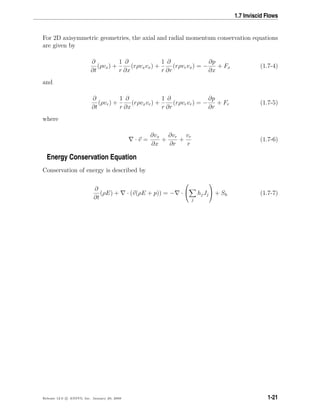
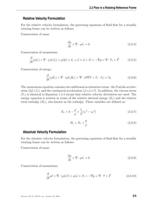
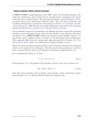
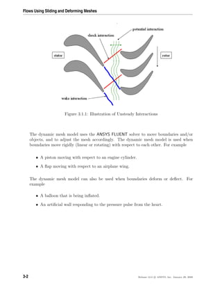
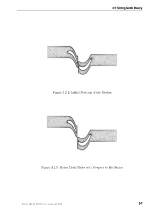
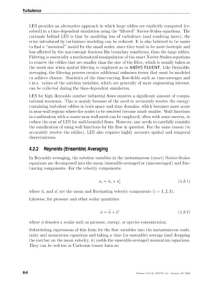
moving domains. However, you can model other types of transients, including translating
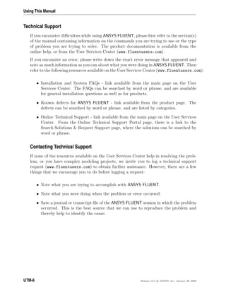
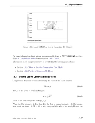
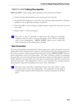
sliding mesh zones (e.g., two cars or trains passing in a tunnel, as shown in Figure 3.2.1).
Interface
Figure 3.2.1: Two Passing Trains in a Tunnel
3-4 Release 12.0 c ANSYS, Inc. January 29, 2009](https://image.slidesharecdn.com/flth-130501182911-phpapp02/85/Flth-72-320.jpg)
![Flows Using Sliding and Deforming Meshes
• rotation about the x-axis (e.g., roll for airplanes)
• rotation about the y-axis (e.g., pitch for airplanes)
• rotation about the z-axis (e.g., yaw for airplanes)
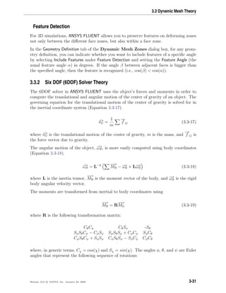
Once the angular and the translational accelerations are computed from Equation 3.3-17
and Equation 3.3-18, the rates are derived by numerical integration [328]. The angular
and translational velocities are used in the dynamic mesh calculations to update the rigid
body position.
3-32 Release 12.0 c ANSYS, Inc. January 29, 2009](https://image.slidesharecdn.com/flth-130501182911-phpapp02/85/Flth-100-320.jpg)
![4.2 Choosing a Turbulence Model
∂ρ
∂t
+
∂
∂xi
(ρui) = 0 (4.2-3)
∂
∂t
(ρui)+
∂
∂xj
(ρuiuj) = −
∂p
∂xi
+
∂
∂xj
µ
∂ui
∂xj
+
∂uj
∂xi
−
2
3
δij
∂ul
∂xl
+
∂
∂xj
(−ρuiuj) (4.2-4)
Equations 4.2-3 and 4.2-4 are called Reynolds-averaged Navier-Stokes (RANS) equations.
They have the same general form as the instantaneous Navier-Stokes equations, with
the velocities and other solution variables now representing ensemble-averaged (or time-
averaged) values. Additional terms now appear that represent the effects of turbulence.
These Reynolds stresses, −ρuiuj, must be modeled in order to close Equation 4.2-4.
For variable-density flows, Equations 4.2-3 and 4.2-4 can be interpreted as Favre-averaged
Navier-Stokes equations [130], with the velocities representing mass-averaged values. As
such, Equations 4.2-3 and 4.2-4 can be applied to density-varying flows.
4.2.3 Boussinesq Approach vs. Reynolds Stress Transport Models
The Reynolds-averaged approach to turbulence modeling requires that the Reynolds
stresses in Equation 4.2-4 are appropriately modeled. A common method employs the
Boussinesq hypothesis [130] to relate the Reynolds stresses to the mean velocity gradients:
− ρuiuj = µt
∂ui
∂xj
+
∂uj
∂xi
−
2
3
ρk + µt
∂uk
∂xk
δij (4.2-5)
The Boussinesq hypothesis is used in the Spalart-Allmaras model, the k- models, and
the k-ω models. The advantage of this approach is the relatively low computational
cost associated with the computation of the turbulent viscosity, µt. In the case of the
Spalart-Allmaras model, only one additional transport equation (representing turbulent
viscosity) is solved. In the case of the k- and k-ω models, two additional transport
equations (for the turbulence kinetic energy, k, and either the turbulence dissipation
rate, , or the specific dissipation rate, ω) are solved, and µt is computed as a function of
k and or k and ω. The disadvantage of the Boussinesq hypothesis as presented is that
it assumes µt is an isotropic scalar quantity, which is not strictly true.
The alternative approach, embodied in the RSM, is to solve transport equations for each
of the terms in the Reynolds stress tensor. An additional scale-determining equation
(normally for ) is also required. This means that five additional transport equations are
required in 2D flows and seven additional transport equations must be solved in 3D.
Release 12.0 c ANSYS, Inc. January 29, 2009 4-5](https://image.slidesharecdn.com/flth-130501182911-phpapp02/85/Flth-105-320.jpg)
![4.3 Spalart-Allmaras Model
In its original form, the Spalart-Allmaras model is effectively a low-Reynolds-number
model, requiring the viscosity-affected region of the boundary layer to be properly re-
solved. In ANSYS FLUENT, however, the Spalart-Allmaras model has been implemented
to use wall functions when the mesh resolution is not sufficiently fine. This might make
it the best choice for relatively crude simulations on coarse meshes where accurate tur-
bulent flow computations are not critical. Furthermore, the near-wall gradients of the
transported variable in the model are much smaller than the gradients of the transported
variables in the k- or k-ω models. This might make the model less sensitive to numer-
ical errors when non-layered meshes are used near walls. See Section 6.1.3: Numerical
Diffusion in the separate User’s Guide for a further discussion of the numerical errors.
On a cautionary note, however, the Spalart-Allmaras model is still relatively new, and
no claim is made regarding its suitability to all types of complex engineering flows. For
instance, it cannot be relied on to predict the decay of homogeneous, isotropic turbu-
lence. Furthermore, one-equation models are often criticized for their inability to rapidly
accommodate changes in length scale, such as might be necessary when the flow changes
abruptly from a wall-bounded to a free shear flow.
In turbulence models that employ the Boussinesq approach, the central issue is how the
eddy viscosity is computed. The model proposed by Spalart and Allmaras [331] solves
a transport equation for a quantity that is a modified form of the turbulent kinematic
viscosity.
4.3.2 Transport Equation for the Spalart-Allmaras Model
The transported variable in the Spalart-Allmaras model, ν, is identical to the turbulent
kinematic viscosity except in the near-wall (viscosity-affected) region. The transport
equation for ν is
∂
∂t
(ρν)+
∂
∂xi
(ρνui) = Gν +
1
σν
∂
∂xj
(µ + ρν)
∂ν
∂xj
+ Cb2ρ
∂ν
∂xj
2
−Yν +Sν (4.3-1)
where Gν is the production of turbulent viscosity, and Yν is the destruction of turbulent
viscosity that occurs in the near-wall region due to wall blocking and viscous damping.
σν and Cb2 are the constants and ν is the molecular kinematic viscosity. Sν is a user-
defined source term. Note that since the turbulence kinetic energy, k, is not calculated
in the Spalart-Allmaras model, while the last term in Equation 4.2-5 is ignored when
estimating the Reynolds stresses.
Release 12.0 c ANSYS, Inc. January 29, 2009 4-7](https://image.slidesharecdn.com/flth-130501182911-phpapp02/85/Flth-107-320.jpg)
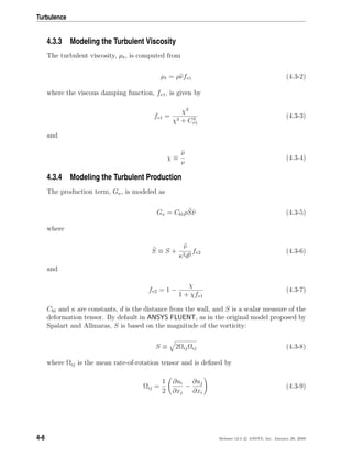
![4.3 Spalart-Allmaras Model
The justification for the default expression for S is that, in the wall-bounded flows that
were of most interest when the model was formulated, the turbulence production found
only where vorticity is generated near walls. However, it has since been acknowledged that
one should also take into account the effect of mean strain on the turbulence production,
and a modification to the model has been proposed [65] and incorporated into ANSYS
FLUENT.
This modification combines the measures of both vorticity and the strain tensors in the
definition of S:
S ≡ |Ωij| + Cprod min (0, |Sij| − |Ωij|) (4.3-10)
where
Cprod = 2.0, |Ωij| ≡ 2ΩijΩij, |Sij| ≡ 2SijSij
with the mean strain rate, Sij, defined as
Sij =
1
2
∂uj
∂xi
+
∂ui
∂xj
(4.3-11)
Including both the rotation and strain tensors reduces the production of eddy viscosity
and consequently reduces the eddy viscosity itself in regions where the measure of vortic-
ity exceeds that of strain rate. One such example can be found in vortical flows, i.e., flow
near the core of a vortex subjected to a pure rotation where turbulence is known to be
suppressed. Including both the rotation and strain tensors more correctly accounts for
the effects of rotation on turbulence. The default option (including the rotation tensor
only) tends to overpredict the production of eddy viscosity and hence overpredicts the
eddy viscosity itself in certain circumstances.
You can select the modified form for calculating production in the Viscous Model dialog
box.
Release 12.0 c ANSYS, Inc. January 29, 2009 4-9](https://image.slidesharecdn.com/flth-130501182911-phpapp02/85/Flth-109-320.jpg)
![Turbulence
4.3.5 Modeling the Turbulent Destruction
The destruction term is modeled as
Yν = Cw1ρfw
ν
d
2
(4.3-12)
where
fw = g
1 + C6
w3
g6 + C6
w3
1/6
(4.3-13)
g = r + Cw2 r6
− r (4.3-14)
r ≡
ν
Sκ2d2
(4.3-15)
Cw1, Cw2, and Cw3 are constants, and S is given by Equation 4.3-6. Note that the
modification described above to include the effects of mean strain on S will also affect
the value of S used to compute r.
4.3.6 Model Constants
The model constants Cb1, Cb2, σν, Cv1, Cw1, Cw2, Cw3, and κ have the following default
values [331]:
Cb1 = 0.1355, Cb2 = 0.622, σν =
2
3
, Cv1 = 7.1
Cw1 =
Cb1
κ2
+
(1 + Cb2)
σν
, Cw2 = 0.3, Cw3 = 2.0, κ = 0.4187
4.3.7 Wall Boundary Conditions
At walls, the modified turbulent kinematic viscosity, ν, is set to zero.
When the mesh is fine enough to resolve the viscosity-dominated sublayer, the wall shear
stress is obtained from the laminar stress-strain relationship:
u
uτ
=
ρuτ y
µ
(4.3-16)
4-10 Release 12.0 c ANSYS, Inc. January 29, 2009](https://image.slidesharecdn.com/flth-130501182911-phpapp02/85/Flth-110-320.jpg)
![4.4 Standard, RNG, and Realizable k- Models
If the mesh is too coarse to resolve the viscous sublayer, then it is assumed that the
centroid of the wall-adjacent cell falls within the logarithmic region of the boundary
layer, and the law-of-the-wall is employed:
u
uτ
=
1
κ
ln E
ρuτ y
µ
(4.3-17)
where u is the velocity parallel to the wall, uτ is the shear velocity, y is the distance from
the wall, κ is the von K´arm´an constant (0.4187), and E = 9.793.
4.3.8 Convective Heat and Mass Transfer Modeling
In ANSYS FLUENT, turbulent heat transport is modeled using the concept of the Reynolds’
analogy to turbulent momentum transfer. The “modeled” energy equation is as follows:
∂
∂t
(ρE) +
∂
∂xi
[ui(ρE + p)] =
∂
∂xj
k +
cpµt
Prt
∂T
∂xj
+ ui(τij)eff + Sh (4.3-18)
where k, in this case, is the thermal conductivity, E is the total energy, and (τij)eff is the
deviatoric stress tensor, defined as
(τij)eff = µeff
∂uj
∂xi
+
∂ui
∂xj
−
2
3
µeff
∂uk
∂xk
δij
4.4 Standard, RNG, and Realizable k- Models
This section describes the theory behind the Standard, RNG, and Realizable k- models.
Information is presented in the following sections:
• Section 4.4.1: Standard k- Model
• Section 4.4.2: RNG k- Model
• Section 4.4.3: Realizable k- Model
• Section 4.4.4: Modeling Turbulent Production in the k- Models
• Section 4.4.5: Effects of Buoyancy on Turbulence in the k- Models
• Section 4.4.6: Effects of Compressibility on Turbulence in the k- Models
• Section 4.4.7: Convective Heat and Mass Transfer Modeling in the k- Models
Release 12.0 c ANSYS, Inc. January 29, 2009 4-11](https://image.slidesharecdn.com/flth-130501182911-phpapp02/85/Flth-111-320.jpg)
![Turbulence
For details about using the models in ANSYS FLUENT, see Chapter 12: Modeling Turbulence
and Section 12.6: Setting Up the k- Model in the separate User’s Guide.
This section presents the standard, RNG, and realizable k- models. All three models
have similar forms, with transport equations for k and . The major differences in the
models are as follows:
• the method of calculating turbulent viscosity
• the turbulent Prandtl numbers governing the turbulent diffusion of k and
• the generation and destruction terms in the equation
The transport equations, the methods of calculating turbulent viscosity, and model con-
stants are presented separately for each model. The features that are essentially common
to all models follow, including turbulent generation due to shear buoyancy, accounting
for the effects of compressibility, and modeling heat and mass transfer.
4.4.1 Standard k- Model
Overview
The simplest “complete models” of turbulence are the two-equation models in which the
solution of two separate transport equations allows the turbulent velocity and length
scales to be independently determined. The standard k- model in ANSYS FLUENT falls
within this class of models and has become the workhorse of practical engineering flow
calculations in the time since it was proposed by Launder and Spalding [180]. Robust-
ness, economy, and reasonable accuracy for a wide range of turbulent flows explain its
popularity in industrial flow and heat transfer simulations. It is a semi-empirical model,
and the derivation of the model equations relies on phenomenological considerations and
empiricism.
As the strengths and weaknesses of the standard k- model have become known, im-
provements have been made to the model to improve its performance. Two of these
variants are available in ANSYS FLUENT: the RNG k- model [384] and the realizable
k- model [313].
The standard k- model [180] is a semi-empirical model based on model transport equa-
tions for the turbulence kinetic energy (k) and its dissipation rate ( ). The model trans-
port equation for k is derived from the exact equation, while the model transport equation
for was obtained using physical reasoning and bears little resemblance to its mathe-
matically exact counterpart.
In the derivation of the k- model, the assumption is that the flow is fully turbulent, and
the effects of molecular viscosity are negligible. The standard k- model is therefore valid
only for fully turbulent flows.
4-12 Release 12.0 c ANSYS, Inc. January 29, 2009](https://image.slidesharecdn.com/flth-130501182911-phpapp02/85/Flth-112-320.jpg)
![4.4 Standard, RNG, and Realizable k- Models
Transport Equations for the Standard k- Model
The turbulence kinetic energy, k, and its rate of dissipation, , are obtained from the
following transport equations:
∂
∂t
(ρk) +
∂
∂xi
(ρkui) =
∂
∂xj
µ +
µt
σk
∂k
∂xj
+ Gk + Gb − ρ − YM + Sk (4.4-1)
and
∂
∂t
(ρ ) +
∂
∂xi
(ρ ui) =
∂
∂xj
µ +
µt
σ
∂
∂xj
+ C1
k
(Gk + C3 Gb) − C2 ρ
2
k
+ S (4.4-2)
In these equations, Gk represents the generation of turbulence kinetic energy due to the
mean velocity gradients, calculated as described in Section 4.4.4: Modeling Turbulent
Production in the k- Models. Gb is the generation of turbulence kinetic energy due
to buoyancy, calculated as described in Section 4.4.5: Effects of Buoyancy on Turbu-
lence in the k- Models. YM represents the contribution of the fluctuating dilatation in
compressible turbulence to the overall dissipation rate, calculated as described in Sec-
tion 4.4.6: Effects of Compressibility on Turbulence in the k- Models. C1 , C2 , and C3
are constants. σk and σ are the turbulent Prandtl numbers for k and , respectively. Sk
and S are user-defined source terms.
Modeling the Turbulent Viscosity
The turbulent (or eddy) viscosity, µt, is computed by combining k and as follows:
µt = ρCµ
k2
(4.4-3)
where Cµ is a constant.
Model Constants
The model constants C1 , C2 , Cµ, σk, and σ have the following default values [180]:
C1 = 1.44, C2 = 1.92, Cµ = 0.09, σk = 1.0, σ = 1.3
These default values have been determined from experiments with air and water for funda-
mental turbulent shear flows including homogeneous shear flows and decaying isotropic
grid turbulence. They have been found to work fairly well for a wide range of wall-
bounded and free shear flows.
Release 12.0 c ANSYS, Inc. January 29, 2009 4-13](https://image.slidesharecdn.com/flth-130501182911-phpapp02/85/Flth-113-320.jpg)
![Turbulence
Although the default values of the model constants are the standard ones most widely
accepted, you can change them (if needed) in the Viscous Model dialog box.
4.4.2 RNG k- Model
Overview
The RNG k- model was derived using a rigorous statistical technique (called renormal-
ization group theory). It is similar in form to the standard k- model, but includes the
following refinements:
• The RNG model has an additional term in its equation that significantly improves
the accuracy for rapidly strained flows.
• The effect of swirl on turbulence is included in the RNG model, enhancing accuracy
for swirling flows.
• The RNG theory provides an analytical formula for turbulent Prandtl numbers,
while the standard k- model uses user-specified, constant values.
• While the standard k- model is a high-Reynolds-number model, the RNG theory
provides an analytically-derived differential formula for effective viscosity that ac-
counts for low-Reynolds-number effects. Effective use of this feature does, however,
depend on an appropriate treatment of the near-wall region.
These features make the RNG k- model more accurate and reliable for a wider class of
flows than the standard k- model.
The RNG-based k- turbulence model is derived from the instantaneous Navier-Stokes
equations, using a mathematical technique called “renormalization group” (RNG) meth-
ods. The analytical derivation results in a model with constants different from those in
the standard k- model, and additional terms and functions in the transport equations
for k and . A more comprehensive description of RNG theory and its application to
turbulence can be found in [259].
4-14 Release 12.0 c ANSYS, Inc. January 29, 2009](https://image.slidesharecdn.com/flth-130501182911-phpapp02/85/Flth-114-320.jpg)
![Turbulence
4.4.3 Realizable k- Model
Overview
The realizable k- model [313] is a relatively recent development and differs from the
standard k- model in two important ways:
• The realizable k- model contains a new formulation for the turbulent viscosity.
• A new transport equation for the dissipation rate, , has been derived from an exact
equation for the transport of the mean-square vorticity fluctuation.
The term “realizable” means that the model satisfies certain mathematical constraints
on the Reynolds stresses, consistent with the physics of turbulent flows. Neither the
standard k- model nor the RNG k- model is realizable.
An immediate benefit of the realizable k- model is that it more accurately predicts
the spreading rate of both planar and round jets. It is also likely to provide superior
performance for flows involving rotation, boundary layers under strong adverse pressure
gradients, separation, and recirculation.
To understand the mathematics behind the realizable k- model, consider combining
the Boussinesq relationship (Equation 4.2-5) and the eddy viscosity definition (Equa-
tion 4.4-3) to obtain the following expression for the normal Reynolds stress in an in-
compressible strained mean flow:
u2 =
2
3
k − 2 νt
∂U
∂x
(4.4-13)
Using Equation 4.4-3 for νt ≡ µt/ρ, one obtains the result that the normal stress, u2,
which by definition is a positive quantity, becomes negative, i.e., “non-realizable”, when
the strain is large enough to satisfy
k ∂U
∂x
>
1
3Cµ
≈ 3.7 (4.4-14)
Similarly, it can also be shown that the Schwarz inequality for shear stresses (uαuβ
2
≤
u2
αu2
β; no summation over α and β) can be violated when the mean strain rate is large.
The most straightforward way to ensure the realizability (positivity of normal stresses
and Schwarz inequality for shear stresses) is to make Cµ variable by sensitizing it to
the mean flow (mean deformation) and the turbulence (k, ). The notion of variable
Cµ is suggested by many modelers including Reynolds [291], and is well substantiated
by experimental evidence. For example, Cµ is found to be around 0.09 in the inertial
sublayer of equilibrium boundary layers, and 0.05 in a strong homogeneous shear flow.
4-18 Release 12.0 c ANSYS, Inc. January 29, 2009](https://image.slidesharecdn.com/flth-130501182911-phpapp02/85/Flth-118-320.jpg)
![4.4 Standard, RNG, and Realizable k- Models
Both the realizable and RNG k- models have shown substantial improvements over the
standard k- model where the flow features include strong streamline curvature, vortices,
and rotation. Since the model is still relatively new, it is not clear in exactly which
instances the realizable k- model consistently outperforms the RNG model. However,
initial studies have shown that the realizable model provides the best performance of all
the k- model versions for several validations of separated flows and flows with complex
secondary flow features.
One of the weaknesses of the standard k- model or other traditional k- models lies with
the modeled equation for the dissipation rate ( ). The well-known round-jet anomaly
(named based on the finding that the spreading rate in planar jets is predicted reasonably
well, but prediction of the spreading rate for axisymmetric jets is unexpectedly poor) is
considered to be mainly due to the modeled dissipation equation.
The realizable k- model proposed by Shih et al. [313] was intended to address these
deficiencies of traditional k- models by adopting the following:
• A new eddy-viscosity formula involving a variable Cµ originally proposed by
Reynolds [291].
• A new model equation for dissipation ( ) based on the dynamic equation of the
mean-square vorticity fluctuation.
One limitation of the realizable k- model is that it produces non-physical turbulent
viscosities in situations when the computational domain contains both rotating and sta-
tionary fluid zones (e.g., multiple reference frames, rotating sliding meshes). This is due
to the fact that the realizable k- model includes the effects of mean rotation in the
definition of the turbulent viscosity (see Equations 4.4-17–4.4-19). This extra rotation
effect has been tested on single rotating reference frame systems and showed superior
behavior over the standard k- model. However, due to the nature of this modification,
its application to multiple reference frame systems should be taken with some caution.
See Section 4.4.3: Modeling the Turbulent Viscosity for information about how to include
or exclude this term from the model.
Release 12.0 c ANSYS, Inc. January 29, 2009 4-19](https://image.slidesharecdn.com/flth-130501182911-phpapp02/85/Flth-119-320.jpg)
![4.4 Standard, RNG, and Realizable k- Models
This model has been extensively validated for a wide range of flows [167, 313], including
rotating homogeneous shear flows, free flows including jets and mixing layers, channel
and boundary layer flows, and separated flows. For all these cases, the performance of
the model has been found to be substantially better than that of the standard k- model.
Especially noteworthy is the fact that the realizable k- model resolves the round-jet
anomaly; i.e., it predicts the spreading rate for axisymmetric jets as well as that for
planar jets.
Modeling the Turbulent Viscosity
As in other k- models, the eddy viscosity is computed from
µt = ρCµ
k2
(4.4-17)
The difference between the realizable k- model and the standard and RNG k- models
is that Cµ is no longer constant. It is computed from
Cµ =
1
A0 + As
kU∗ (4.4-18)
where
U∗
≡ SijSij + ΩijΩij (4.4-19)
and
Ωij = Ωij − 2 ijkωk
Ωij = Ωij − ijkωk
where Ωij is the mean rate-of-rotation tensor viewed in a rotating reference frame with
the angular velocity ωk. The model constants A0 and As are given by
A0 = 4.04, As =
√
6 cos φ
where
φ =
1
3
cos−1
(
√
6W), W =
SijSjkSki
S3
, S = SijSij, Sij =
1
2
∂uj
∂xi
+
∂ui
∂xj
Release 12.0 c ANSYS, Inc. January 29, 2009 4-21](https://image.slidesharecdn.com/flth-130501182911-phpapp02/85/Flth-121-320.jpg)
![4.4 Standard, RNG, and Realizable k- Models
4.4.5 Effects of Buoyancy on Turbulence in the k- Models
When a non-zero gravity field and temperature gradient are present simultaneously, the
k- models in ANSYS FLUENT account for the generation of k due to buoyancy (Gb in
Equations 4.4-1, 4.4-4, and 4.4-15), and the corresponding contribution to the production
of in Equations 4.4-2, 4.4-5, and 4.4-16.
The generation of turbulence due to buoyancy is given by
Gb = βgi
µt
Prt
∂T
∂xi
(4.4-23)
where Prt is the turbulent Prandtl number for energy and gi is the component of the
gravitational vector in the ith direction. For the standard and realizable k- models,
the default value of Prt is 0.85. In the case of the RNG k- model, Prt = 1/α, where
α is given by Equation 4.4-9, but with α0 = 1/Pr = k/µcp. The coefficient of thermal
expansion, β, is defined as
β = −
1
ρ
∂ρ
∂T p
(4.4-24)
For ideal gases, Equation 4.4-23 reduces to
Gb = −gi
µt
ρPrt
∂ρ
∂xi
(4.4-25)
It can be seen from the transport equations for k (Equations 4.4-1, 4.4-4, and 4.4-15)
that turbulence kinetic energy tends to be augmented (Gb > 0) in unstable stratification.
For stable stratification, buoyancy tends to suppress the turbulence (Gb < 0). In ANSYS
FLUENT, the effects of buoyancy on the generation of k are always included when you
have both a non-zero gravity field and a non-zero temperature (or density) gradient.
While the buoyancy effects on the generation of k are relatively well understood, the
effect on is less clear. In ANSYS FLUENT, by default, the buoyancy effects on are
neglected simply by setting Gb to zero in the transport equation for (Equation 4.4-2,
4.4-5, or 4.4-16).
However, you can include the buoyancy effects on in the Viscous Model dialog box.
In this case, the value of Gb given by Equation 4.4-25 is used in the transport equation
for (Equation 4.4-2, 4.4-5, or 4.4-16).
The degree to which is affected by the buoyancy is determined by the constant C3 . In
ANSYS FLUENT, C3 is not specified, but is instead calculated according to the following
relation [127]:
Release 12.0 c ANSYS, Inc. January 29, 2009 4-23](https://image.slidesharecdn.com/flth-130501182911-phpapp02/85/Flth-123-320.jpg)
![Turbulence
C3 = tanh
v
u
(4.4-26)
where v is the component of the flow velocity parallel to the gravitational vector and
u is the component of the flow velocity perpendicular to the gravitational vector. In
this way, C3 will become 1 for buoyant shear layers for which the main flow direction is
aligned with the direction of gravity. For buoyant shear layers that are perpendicular to
the gravitational vector, C3 will become zero.
4.4.6 Effects of Compressibility on Turbulence in the k- Models
For high-Mach-number flows, compressibility affects turbulence through so-called “di-
latation dissipation”, which is normally neglected in the modeling of incompressible
flows [379]. Neglecting the dilatation dissipation fails to predict the observed decrease in
spreading rate with increasing Mach number for compressible mixing and other free shear
layers. To account for these effects in the k- models in ANSYS FLUENT, the dilatation
dissipation term, YM , is included in the k equation. This term is modeled according to
a proposal by Sarkar [300]:
YM = 2ρ M2
t (4.4-27)
where Mt is the turbulent Mach number, defined as
Mt =
k
a2
(4.4-28)
where a (≡
√
γRT) is the speed of sound.
This compressibility modification always takes effect when the compressible form of the
ideal gas law is used.
4.4.7 Convective Heat and Mass Transfer Modeling in the k- Models
In ANSYS FLUENT, turbulent heat transport is modeled using the concept of Reynolds’
analogy to turbulent momentum transfer. The “modeled” energy equation is thus given
by the following:
∂
∂t
(ρE) +
∂
∂xi
[ui(ρE + p)] =
∂
∂xj
keff
∂T
∂xj
+ ui(τij)eff + Sh (4.4-29)
where E is the total energy, keff is the effective thermal conductivity, and
(τij)eff is the deviatoric stress tensor, defined as
4-24 Release 12.0 c ANSYS, Inc. January 29, 2009](https://image.slidesharecdn.com/flth-130501182911-phpapp02/85/Flth-124-320.jpg)
![4.4 Standard, RNG, and Realizable k- Models
(τij)eff = µeff
∂uj
∂xi
+
∂ui
∂xj
−
2
3
µeff
∂uk
∂xk
δij
The term involving (τij)eff represents the viscous heating, and is always computed in the
density-based solvers. It is not computed by default in the pressure-based solver, but it
can be enabled in the Viscous Model dialog box.
Additional terms may appear in the energy equation, depending on the physical models
you are using. See Section 5.2.1: Heat Transfer Theory for more details.
For the standard and realizable k- models, the effective thermal conductivity is given
by
keff = k +
cpµt
Prt
where k, in this case, is the thermal conductivity. The default value of the turbulent
Prandtl number is 0.85. You can change the value of the turbulent Prandtl number in
the Viscous Model dialog box.
For the RNG k- model, the effective thermal conductivity is
keff = αcpµeff
where α is calculated from Equation 4.4-9, but with α0 = 1/Pr = k/µcp.
The fact that α varies with µmol/µeff, as in Equation 4.4-9, is an advantage of the RNG k-
model. It is consistent with experimental evidence indicating that the turbulent Prandtl
number varies with the molecular Prandtl number and turbulence [159]. Equation 4.4-9
works well across a very broad range of molecular Prandtl numbers, from liquid metals
(Pr ≈ 10−2
) to paraffin oils (Pr ≈ 103
), which allows heat transfer to be calculated in
low-Reynolds-number regions. Equation 4.4-9 smoothly predicts the variation of effective
Prandtl number from the molecular value (α = 1/Pr) in the viscosity-dominated region
to the fully turbulent value (α = 1.393) in the fully turbulent regions of the flow.
Turbulent mass transfer is treated similarly. For the standard and realizable k- models,
the default turbulent Schmidt number is 0.7. This default value can be changed in the
Viscous Model dialog box. For the RNG model, the effective turbulent diffusivity for
mass transfer is calculated in a manner that is analogous to the method used for the heat
transport. The value of α0 in Equation 4.4-9 is α0 = 1/Sc, where Sc is the molecular
Schmidt number.
Release 12.0 c ANSYS, Inc. January 29, 2009 4-25](https://image.slidesharecdn.com/flth-130501182911-phpapp02/85/Flth-125-320.jpg)
![Turbulence
4.5 Standard and SST k-ω Models
This section describes the theory behind the Standard and SST k-ω model. Information
is presented in the following sections:
• Section 4.5.1: Standard k-ω Model
• Section 4.5.2: Shear-Stress Transport (SST) k-ω Model
• Section 4.5.3: Wall Boundary Conditions
For details about using the models in ANSYS FLUENT, see Chapter 12: Modeling Turbulence
and Section 12.7: Setting Up the k-ω Model in the separate User’s Guide.
This section presents the standard [379] and shear-stress transport (SST) [224] k-ω mod-
els. Both models have similar forms, with transport equations for k and ω. The major
ways in which the SST model [225] differs from the standard model are as follows:
• gradual change from the standard k-ω model in the inner region of the boundary
layer to a high-Reynolds-number version of the k- model in the outer part of the
boundary layer
• modified turbulent viscosity formulation to account for the transport effects of the
principal turbulent shear stress
The transport equations, methods of calculating turbulent viscosity, and methods of
calculating model constants and other terms are presented separately for each model.
4.5.1 Standard k-ω Model
Overview
The standard k-ω model in ANSYS FLUENT is based on the Wilcox k-ω model [379],
which incorporates modifications for low-Reynolds-number effects, compressibility, and
shear flow spreading. The Wilcox model predicts free shear flow spreading rates that are
in close agreement with measurements for far wakes, mixing layers, and plane, round,
and radial jets, and is thus applicable to wall-bounded flows and free shear flows. A
variation of the standard k-ω model called the SST k-ω model is also available in ANSYS
FLUENT, and is described in Section 4.5.2: Shear-Stress Transport (SST) k-ω Model.
The standard k-ω model is an empirical model based on model transport equations for
the turbulence kinetic energy (k) and the specific dissipation rate (ω), which can also be
thought of as the ratio of to k [379].
As the k-ω model has been modified over the years, production terms have been added
to both the k and ω equations, which have improved the accuracy of the model for
predicting free shear flows.
4-26 Release 12.0 c ANSYS, Inc. January 29, 2009](https://image.slidesharecdn.com/flth-130501182911-phpapp02/85/Flth-126-320.jpg)
![4.5 Standard and SST k-ω Models
Production of ω
The production of ω is given by
Gω = α
ω
k
Gk (4.5-13)
where Gk is given by Equation 4.5-11.
The coefficient α is given by
α =
α∞
α∗
α0 + Ret/Rω
1 + Ret/Rω
(4.5-14)
where Rω = 2.95. α∗
and Ret are given by Equations 4.5-6 and 4.5-7, respectively.
Note that, in the high-Reynolds-number form of the k-ω model, α = α∞ = 1.
Modeling the Turbulence Dissipation
Dissipation of k
The dissipation of k is given by
Yk = ρ β∗
fβ∗ k ω (4.5-15)
where
fβ∗ =
1 χk ≤ 0
1+680χ2
k
1+400χ2
k
χk > 0
(4.5-16)
where
χk ≡
1
ω3
∂k
∂xj
∂ω
∂xj
(4.5-17)
and
β∗
= β∗
i [1 + ζ∗
F(Mt)] (4.5-18)
β∗
i = β∗
∞
4/15 + (Ret/Rβ)4
1 + (Ret/Rβ)4
(4.5-19)
ζ∗
= 1.5 (4.5-20)
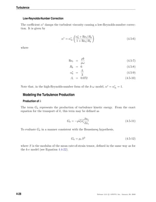
Release 12.0 c ANSYS, Inc. January 29, 2009 4-29](https://image.slidesharecdn.com/flth-130501182911-phpapp02/85/Flth-129-320.jpg)
![4.5 Standard and SST k-ω Models
Note that, in the high-Reynolds-number form of the k-ω model, β∗
i = β∗
∞. In the incom-
pressible form, β∗
= β∗
i .
Model Constants
α∗
∞ = 1, α∞ = 0.52, α0 =
1
9
, β∗
∞ = 0.09, βi = 0.072, Rβ = 8
Rk = 6, Rω = 2.95, ζ∗
= 1.5, Mt0 = 0.25, σk = 2.0, σω = 2.0
4.5.2 Shear-Stress Transport (SST) k-ω Model
Overview
The shear-stress transport (SST) k-ω model was developed by Menter [224] to effectively
blend the robust and accurate formulation of the k-ω model in the near-wall region with
the free-stream independence of the k- model in the far field. To achieve this, the k-
model is converted into a k-ω formulation. The SST k-ω model is similar to the standard
k-ω model, but includes the following refinements:
• The standard k-ω model and the transformed k- model are both multiplied by a
blending function and both models are added together. The blending function is
designed to be one in the near-wall region, which activates the standard k-ω model,
and zero away from the surface, which activates the transformed k- model.
• The SST model incorporates a damped cross-diffusion derivative term in the ω
equation.
• The definition of the turbulent viscosity is modified to account for the transport of
the turbulent shear stress.
• The modeling constants are different.
These features make the SST k-ω model more accurate and reliable for a wider class
of flows (e.g., adverse pressure gradient flows, airfoils, transonic shock waves) than the
standard k-ω model. Other modifications include the addition of a cross-diffusion term
in the ω equation and a blending function to ensure that the model equations behave
appropriately in both the near-wall and far-field zones.
Release 12.0 c ANSYS, Inc. January 29, 2009 4-31](https://image.slidesharecdn.com/flth-130501182911-phpapp02/85/Flth-131-320.jpg)
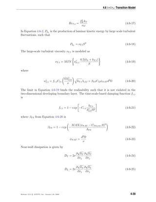
![4.6 k-kl-ω Transition Model
4.6 k-kl-ω Transition Model
This section describes the theory behind the k-kl-ω Transition model. For details about
using the model in ANSYS FLUENT, see Chapter 12: Modeling Turbulence and Sec-
tion 12.8: Setting Up the Transition k-kl-ω Model in the separate User’s Guide.
4.6.1 Overview
The k-kl-ω transition model [364] is used to predict boundary layer development and
calculate transition onset. This model can be used to effectively address the transition
of the boundary layer from a laminar to a turbulent regime.
4.6.2 Transport Equations for the k-kl-ω Model
The k-kl-ω model is considered to be a three-equation eddy-viscosity type, which includes
transport equations for turbulent kinetic energy (kT ), laminar kinetic energy (kL), and
the inverse turbulent time scale (ω)
DkT
Dt
= PKT
+ R + RNAT − ωkT − DT +
∂
∂xj
ν +
αT
αk
∂kT
∂xj
(4.6-1)
DkL
Dt
= PKL
− R − RNAT − DL +
∂
∂xj
ν
∂kL
∂xj
(4.6-2)
Dω
Dt
= Cω1
ω
kT
PkT
+
CωR
fW
− 1
ω
kT
(R+RNAT )−Cω2ω2
+Cω3fωαT f2
W
√
kT
d3
+
∂
∂xj
ν +
αT
αω
∂ω
∂xj
(4.6-3)
The inclusion of the turbulent and laminar fluctuations on the mean flow and energy
equations via the eddy viscosity and total thermal diffusivity is as follows:
−uiuj = νTOT
∂Ui
∂xj
+
∂Uj
∂xi
−
2
3
kTOT δij (4.6-4)
−uiθ = αθ,TOT
∂θ
∂xi
(4.6-5)
The effective length is defined as
λeff = MIN(Cλd, λT ) (4.6-6)
where λT is the turbulent length scale and is defined by
Release 12.0 c ANSYS, Inc. January 29, 2009 4-37](https://image.slidesharecdn.com/flth-130501182911-phpapp02/85/Flth-137-320.jpg)
![4.7 Transition SST Model
αT = fνCµ,std kT,sλeff (4.6-35)
kTOT = kT + kL (4.6-36)
Model Constants
The model constants for the k-kl-ω transition model are listed below [364]
A0 = 4.04, As = 2.12, Aν = 6.75, ABP = 0.6
ANAT = 200, ATS = 200, CBP,crit = 1.2, CNC = 0.1
CNAT,crit = 1250, CINT = 0.75, CTS,crit = 1000, CR,NAT = 0.02
C11 = 3.4 × 10⁻⁶
, C12 = 1.0 × 10⁻¹⁰
, CR = 0.12, Cα,θ = 0.035
CSS = 1.5, Cτ,1 = 4360, Cω1 = 0.44, Cω2 = 0.92
Cω3 = 0.3, CωR = 1.5, Cλ = 2.495, Cµ,std = 0.09
Prθ = 0.85, σk = 1, σω = 1.17
4.7 Transition SST Model
This section describes the theory behind the Transition SST model. Information is
presented in the following sections:
• Section 4.7.1: Overview
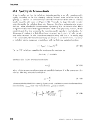
• Section 4.7.2: Transport Equations for the Transition SST Model
• Section 4.7.3: Specifying Inlet Turbulence Levels
For details about using the model in ANSYS FLUENT, see Chapter 12: Modeling Turbulence
and Section 12.9: Setting Up the Transition SST Model in the separate User’s Guide.
Release 12.0 c ANSYS, Inc. January 29, 2009 4-41](https://image.slidesharecdn.com/flth-130501182911-phpapp02/85/Flth-141-320.jpg)
![Turbulence
4.7.1 Overview
The transition SST model is based on the coupling of the SST k − ω transport equations
with two other transport equations, one for the intermittency and one for the transition
onset criteria, in terms of momentum-thickness Reynolds number. An ANSYS proprietary
empirical correlation (Langtry and Menter) has been developed to cover standard bypass
transition as well as flows in low free-stream turbulence environments.
In addition, a very powerful option has been included to allow you to enter your own
user-defined empirical correlation, which can then be used to control the transition onset
momentum thickness Reynolds number equation. To learn how to set up the transition
SST model, see Section 12.9: Setting Up the Transition SST Model (in the separate User’s
Guide).
4.7.2 Transport Equations for the Transition SST Model
The transport equation for the intermittency γ is defined as:
∂(ργ)
∂t
+
∂(ρUjγ)
∂xj
= Pγ1 − Eγ1 + Pγ2 − Eγ2 +
∂
∂xj
µ +
µt
σγ
∂γ
∂xj
(4.7-1)
The transition sources are defined as follows:
Pγ1 = 2FlengthρS[γFonset]cγ3
Eγ1 = Pγ1γ (4.7-2)
where S is the strain rate magnitude. Flength is an empirical correlation that controls the
length of the transition region. The destruction/relaminarization sources are defined as
follows:
Pγ2 = (2cγ1)ρΩγFturb
Eγ2 = cγ2Pγ2γ (4.7-3)
where Ω is the vorticity magnitude. The transition onset is controlled by the following
functions:
ReV =
ρy2
S
µ
RT =
ρk
µω
(4.7-4)
4-42 Release 12.0 c ANSYS, Inc. January 29, 2009](https://image.slidesharecdn.com/flth-130501182911-phpapp02/85/Flth-142-320.jpg)
![4.7 Transition SST Model
Fonset1 =
Rev
2.193Reθc
Fonset2 = min(max(Fonset1, F4
onset1), 2.0) (4.7-5)
Fonset3 = max 1 −
RT
2.5
3
, 0
Fonset = max(Fonset2 − Fonset3, 0)
Fturb = e
−
RT
4
4
(4.7-6)
Reθc is the critical Reynolds number where the intermittency first starts to increase in
the boundary layer. This occurs upstream of the transition Reynolds number Reθt and
the difference between the two must be obtained from an empirical correlation. Both the
Flength and Reθc correlations are functions of Reθt.
The constants for the intermittency equation are:
cγ1 = 0.03; cγ2 = 50; cγ3 = 0.5; σγ = 1.0
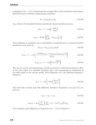
Separation Induced Transition Correction
The modification for separation-induced transition is:
γsep = min 2max
Rev
3.235Reθc
− 1, 0 Freattch, 2 Fθt
Freattch = e
−
RT
20
4
γeff = max(γ, γsep) (4.7-7)
The model constants in Equation 4.7-7 have been adjusted from those of Menter et
al. [226] in order to improve the predictions of separated flow transition. The main
difference is that the constant that controls the relation between Rev and Reθc was
changed from 2.193, its value for a Blasius boundary layer, to 3.235, the value at a
separation point where the shape factor is 3.5 [226]. The boundary condition for γ at a
wall is zero normal flux, while for an inlet, γ is equal to 1.0.
The transport equation for the transition momentum thickness Reynolds number Reθt is
∂(ρReθt)
∂t
+
∂(ρUjReθt)
∂xj
= Pθt +
∂
∂xj
σθt(µ + µt)
∂Reθt
∂xj
(4.7-8)
Release 12.0 c ANSYS, Inc. January 29, 2009 4-43](https://image.slidesharecdn.com/flth-130501182911-phpapp02/85/Flth-143-320.jpg)
![Turbulence
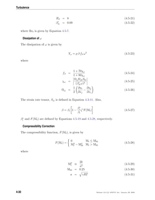
The source term is defined as follows:
Pθt = cθt
ρ
t
(Reθt − Reθt)(1.0 − Fθt)
t =
500µ
ρU2
(4.7-9)
Fθt = min
max
Fwakee(− y
δ )
4
, 1.0 −
γ − 1/50
1.0 − 1/50
2
, 1.0
(4.7-10)
θBL =
Reθtµ
ρU
δBL =
15
2
θBL (4.7-11)
δ =
50Ωy
U
δBL
Reω =
ρωy2
µ
Fwake = e−( Reω
1E+5 )
2
(4.7-12)
The model constants for the Reθt equation are:
cθt = 0.03 σθt = 2.0
The boundary condition for Reθt at a wall is zero flux. The boundary condition for
Reθt at an inlet should be calculated from the empirical correlation based on the inlet
turbulence intensity.
The model contains three empirical correlations. ReΘt is the transition onset as observed
in experiments. This has been modified from Menter et al. [226] in order to improve the
predictions for natural transition. It is used in Equation 4.7-9. Flength is the length of the
transition zone and is substituted in Equation 4.7-2. ReΘc is the point where the model
is activated in order to match both ReΘt and Flength, and is used in Equation 4.7-5. At
present, these empirical correlations are proprietary and are not given in this manual.
ReΘt = f(Tu, λ)
Flength = f(ReΘt)
ReΘc = f(ReΘt) (4.7-13)
4-44 Release 12.0 c ANSYS, Inc. January 29, 2009](https://image.slidesharecdn.com/flth-130501182911-phpapp02/85/Flth-144-320.jpg)
![4.7 Transition SST Model
The first empirical correlation is a function of the local turbulence intensity, Tu, and the
Thwaites’ pressure gradient coefficient λθ is defined as
λθ = (θ2
/v)dU/ds (4.7-14)
where dU/ds is the acceleration in the streamwise direction.
Coupling the Transition Model and SST Transport Equations
The transition model interacts with the SST turbulence model, as follows:
∂
∂t
(ρk) +
∂
∂xj
(ρujk) = Pk − Dk +
∂
∂xj
(µ + σkµt)
∂k
∂xj
(4.7-15)
Pk = γeff Pk (4.7-16)
Dk = min(max(γeff , 0.1), 1.0)Dk (4.7-17)
Ry =
ρy
√
k
µ
(4.7-18)
F3 = e− Ry
120
3
(4.7-19)
Ft = max(F1orig, F3) (4.7-20)
where Pk and Dk are the original production and destruction terms for the SST model
and F1orig is the original SST blending function. Note that the production term in the
ω-equation is not modified. The rationale behind the above model formulation is given
in detail in Menter et al. [226].
In order to capture the laminar and transitional boundary layers correctly, the mesh must
have a y+
of approximately one. If the y+
is too large (i.e. > 5), then the transition
onset location moves upstream with increasing y+
. It is recommended to use the bounded
second order upwind based discretization for the mean flow, turbulence and transition
equations.
Release 12.0 c ANSYS, Inc. January 29, 2009 4-45](https://image.slidesharecdn.com/flth-130501182911-phpapp02/85/Flth-145-320.jpg)
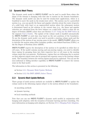
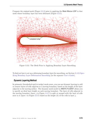
![4.8 The v2
-f Model
Figure 4.7.1: Decay of Turbulence Intensity (Tu) as a Function of Streamwise
Distance (x)
4.8 The v2
-f Model
The v2
-f model is similar to the standard k- model, but incorporates near-wall turbu-
lence anisotropy and non-local pressure-strain effects. A limitation of the v2
-f model is
that it cannot be used to solve Eulerian multiphase problems, whereas the k- model is
typically used in such applications. The v2
-f model is a general low-Reynolds-number
turbulence model that is valid all the way up to solid walls, and therefore does not need
to make use of wall functions. Although the model was originally developed for attached
or mildly separated boundary layers [82], it also accurately simulates flows dominated by
separation [24].
The distinguishing feature of the v2
-f model is its use of the velocity scale, v2, instead
of the turbulent kinetic energy, k, for evaluating the eddy viscosity. v2, which can be
thought of as the velocity fluctuation normal to the streamlines, has shown to provide
the right scaling in representing the damping of turbulent transport close to the wall, a
feature that k does not provide.
For more information about the theoretical background and usage of the v2
-f model,
please visit the User Services Center (www.fluentusers.com) .
Release 12.0 c ANSYS, Inc. January 29, 2009 4-47](https://image.slidesharecdn.com/flth-130501182911-phpapp02/85/Flth-147-320.jpg)
![Turbulence
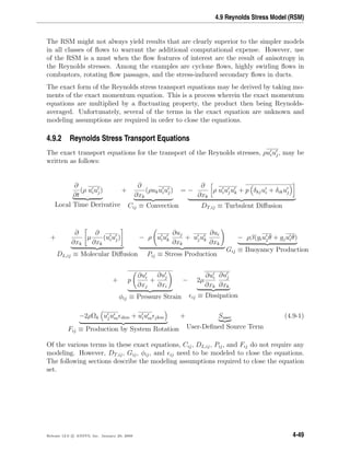
4.9 Reynolds Stress Model (RSM)
This section describes the theory behind the Reynolds Stress model (RSM). Information
is presented in the following sections:
• Section 4.9.1: Overview
• Section 4.9.2: Reynolds Stress Transport Equations
• Section 4.9.3: Modeling Turbulent Diffusive Transport
• Section 4.9.4: Modeling the Pressure-Strain Term
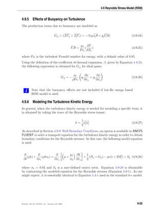
• Section 4.9.5: Effects of Buoyancy on Turbulence
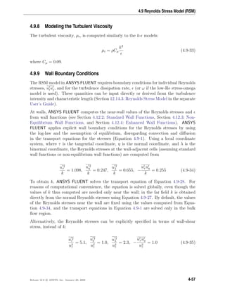
• Section 4.9.6: Modeling the Turbulence Kinetic Energy
• Section 4.9.7: Modeling the Dissipation Rate
• Section 4.9.8: Modeling the Turbulent Viscosity
• Section 4.9.9: Wall Boundary Conditions
• Section 4.9.10: Convective Heat and Mass Transfer Modeling
For details about using the model in ANSYS FLUENT, see Chapter 12: Modeling Turbulence
and Section 12.10: Setting Up the Reynolds Stress Model in the separate User’s Guide.
4.9.1 Overview
The Reynolds stress model (RSM) [108, 177, 178] is the most elaborate type of turbu-
lence model that ANSYS FLUENT provides. Abandoning the isotropic eddy-viscosity
hypothesis, the RSM closes the Reynolds-averaged Navier-Stokes equations by solving
transport equations for the Reynolds stresses, together with an equation for the dissipa-
tion rate. This means that five additional transport equations are required in 2D flows,
in comparison to seven additional transport equations solved in 3D.
Since the RSM accounts for the effects of streamline curvature, swirl, rotation, and rapid
changes in strain rate in a more rigorous manner than one-equation and two-equation
models, it has greater potential to give accurate predictions for complex flows. However,
the fidelity of RSM predictions is still limited by the closure assumptions employed to
model various terms in the exact transport equations for the Reynolds stresses. The
modeling of the pressure-strain and dissipation-rate terms is particularly challenging, and
often considered to be responsible for compromising the accuracy of RSM predictions.
4-48 Release 12.0 c ANSYS, Inc. January 29, 2009](https://image.slidesharecdn.com/flth-130501182911-phpapp02/85/Flth-148-320.jpg)
![Turbulence
4.9.3 Modeling Turbulent Diffusive Transport
DT,ij can be modeled by the generalized gradient-diffusion model of Daly and Harlow [67]:
DT,ij = Cs
∂
∂xk
ρ
kuku ∂uiuj
∂x
(4.9-2)
However, this equation can result in numerical instabilities, so it has been simplified in
ANSYS FLUENT to use a scalar turbulent diffusivity as follows [194]:
DT,ij =
∂
∂xk
µt
σk
∂uiuj
∂xk
(4.9-3)
The turbulent viscosity, µt, is computed using Equation 4.9-33.
Lien and Leschziner [194] derived a value of σk = 0.82 by applying the generalized
gradient-diffusion model, Equation 4.9-2, to the case of a planar homogeneous shear
flow. Note that this value of σk is different from that in the standard and realizable k-
models, in which σk = 1.0.
4.9.4 Modeling the Pressure-Strain Term
Linear Pressure-Strain Model
By default in ANSYS FLUENT, the pressure-strain term, φij, in Equation 4.9-1 is modeled
according to the proposals by Gibson and Launder [108], Fu et al. [104], and Launder [176,
177].
The classical approach to modeling φij uses the following decomposition:
φij = φij,1 + φij,2 + φij,w (4.9-4)
where φij,1 is the slow pressure-strain term, also known as the return-to-isotropy term,
φij,2 is called the rapid pressure-strain term, and φij,w is the wall-reflection term.
The slow pressure-strain term, φij,1, is modeled as
φij,1 ≡ −C1ρ
k
uiuj −
2
3
δijk (4.9-5)
with C1 = 1.8.
The rapid pressure-strain term, φij,2, is modeled as
4-50 Release 12.0 c ANSYS, Inc. January 29, 2009](https://image.slidesharecdn.com/flth-130501182911-phpapp02/85/Flth-150-320.jpg)
![4.9 Reynolds Stress Model (RSM)
φij,2 ≡ −C2 (Pij + Fij + 5/6Gij − Cij) −
2
3
δij(P + 5/6G − C) (4.9-6)
where C2 = 0.60, Pij, Fij, Gij, and Cij are defined as in Equation 4.9-1, P = 1
2
Pkk,
G = 1
2
Gkk, and C = 1
2
Ckk.
The wall-reflection term, φij,w, is responsible for the redistribution of normal stresses near
the wall. It tends to damp the normal stress perpendicular to the wall, while enhancing
the stresses parallel to the wall. This term is modeled as
φij,w ≡ C1
k
ukumnknmδij −
3
2
uiuknjnk −
3
2
ujuknink
C k3/2
d
+ C2 φkm,2nknmδij −
3
2
φik,2njnk −
3
2
φjk,2nink
C k3/2
d
(4.9-7)
where C1 = 0.5, C2 = 0.3, nk is the xk component of the unit normal to the wall, d is
the normal distance to the wall, and C = C3/4
µ /κ, where Cµ = 0.09 and κ is the von
K´arm´an constant (= 0.4187).
φij,w is included by default in the Reynolds stress model.
Low-Re Modifications to the Linear Pressure-Strain Model
When the RSM is applied to near-wall flows using the enhanced wall treatment described
in Section 4.12.4: Two-Layer Model for Enhanced Wall Treatment, the pressure-strain
model needs to be modified. The modification used in ANSYS FLUENT specifies the
values of C1, C2, C1, and C2 as functions of the Reynolds stress invariants and the
turbulent Reynolds number, according to the suggestion of Launder and Shima [179]:
C1 = 1 + 2.58AA2
0.25
1 − exp −(0.0067Ret)2
(4.9-8)
C2 = 0.75
√
A (4.9-9)
C1 = −
2
3
C1 + 1.67 (4.9-10)
C2 = max
2
3
C2 − 1
6
C2
, 0 (4.9-11)
with the turbulent Reynolds number defined as Ret = (ρk2
/µ ). The flatness parameter
A and tensor invariants, A2 and A3, are defined as
Release 12.0 c ANSYS, Inc. January 29, 2009 4-51](https://image.slidesharecdn.com/flth-130501182911-phpapp02/85/Flth-151-320.jpg)
![Turbulence
A ≡ 1 −
9
8
(A2 − A3) (4.9-12)
A2 ≡ aikaki (4.9-13)
A3 ≡ aikakjaji (4.9-14)
aij is the Reynolds-stress anisotropy tensor, defined as
aij = −
−ρuiuj + 2
3
ρkδij
ρk
(4.9-15)
The modifications detailed above are employed only when the enhanced wall treatment
is selected in the Viscous Model dialog box.
Quadratic Pressure-Strain Model
An optional pressure-strain model proposed by Speziale, Sarkar, and Gatski [334] is
provided in ANSYS FLUENT. This model has been demonstrated to give superior perfor-
mance in a range of basic shear flows, including plane strain, rotating plane shear, and
axisymmetric expansion/contraction. This improved accuracy should be beneficial for a
wider class of complex engineering flows, particularly those with streamline curvature.
The quadratic pressure-strain model can be selected as an option in the Viscous Model
dialog box.
This model is written as follows:
φij = − (C1ρ + C∗
1 P) bij + C2ρ bikbkj −
1
3
bmnbmnδij + C3 − C∗
3 bijbij ρkSij
+ C4ρk bikSjk + bjkSik −
2
3
bmnSmnδij + C5ρk (bikΩjk + bjkΩik) (4.9-16)
where bij is the Reynolds-stress anisotropy tensor defined as
bij = −
−ρuiuj + 2
3
ρkδij
2ρk
(4.9-17)
The mean strain rate, Sij, is defined as
Sij =
1
2
∂uj
∂xi
+
∂ui
∂xj
(4.9-18)
4-52 Release 12.0 c ANSYS, Inc. January 29, 2009](https://image.slidesharecdn.com/flth-130501182911-phpapp02/85/Flth-152-320.jpg)
![4.9 Reynolds Stress Model (RSM)
The mean rate-of-rotation tensor, Ωij, is defined by
Ωij =
1
2
∂ui
∂xj
−
∂uj
∂xi
(4.9-19)
The constants are
C1 = 3.4, C∗
1 = 1.8, C2 = 4.2, C3 = 0.8, C∗
3 = 1.3, C4 = 1.25, C5 = 0.4
The quadratic pressure-strain model does not require a correction to account for the
wall-reflection effect in order to obtain a satisfactory solution in the logarithmic region
of a turbulent boundary layer. It should be noted, however, that the quadratic pressure-
strain model is not available when the enhanced wall treatment is selected in the Viscous
Model dialog box.
Low-Re Stress-Omega Model
The low-Re stress-omega model is a stress-transport model that is based on the omega
equations and LRR model [379]. This model is ideal for modeling flows over curved sur-
faces and swirling flows. The low-Re stress-omega model can be selected in the Viscous
Model dialog box and requires no treatments of wall reflections. The closure coeffi-
cients are identical to the k-ω model (Section 4.5.1: Model Constants), however, there
are additional closure coefficients, C1 and C2, noted below.
The low-Re stress-omega model resembles the k-ω model due to its excellent predictions
for a wide range of turbulent flows. Furthermore, low Reynolds number modifications
and surface boundary conditions for rough surfaces are similar to the k-ω model.
Equation 4.9-4 can be re-written for the low-Re stress-omega model such that wall re-
flections are excluded:
φij = φij,1 + φij,2 (4.9-20)
Therefore,
φij = −C1ρβ∗
RSM ω ui uj − 2/3δijk − ˆα0 [Pij − 1/3Pkkδij]
− ˆβ0 [Dij − 1/3Pkkδij] − k ˆγ0 [Sij − 1/3Skkδij] (4.9-21)
where Dij is defined as
Release 12.0 c ANSYS, Inc. January 29, 2009 4-53](https://image.slidesharecdn.com/flth-130501182911-phpapp02/85/Flth-153-320.jpg)
![Turbulence
Dij = −ρ ui um
∂um
∂xj
+ uj um
∂um
∂xi
(4.9-22)
The mean strain rate Sij is defined in Equation 4.9-18 and β∗
RSM is defined by
β∗
RSM = β∗
fβ∗ (4.9-23)
where β∗
and f∗
β are defined in the same way as for the standard k − ω, using Equa-
tions 4.5-16 and 4.5-22, respectively. The only difference here is that the equation for f∗
β
uses a value of 640 instead of 680, as in Equation 4.5-16.
The constants are
ˆα0 =
8 + C2
11
, ˆβ0 =
8C2 − 2
11
, ˆγ0 =
60C2 − 4
55
C1 = 1.8, C2 = 0.52
The above formulation does not require viscous damping functions to resolve the near-
wall sublayer. However, inclusion of the viscous damping function [379] could improve
model predictions for certain flows. This results in the following changes:
ˆα =
1 + ˆα0ReT /Rk
1 + ReT /Rk
ˆβ = ˆβ0
ReT /Rk
1 + ReT /Rk
ˆγ = ˆγ0
0.007 + ReT /Rk
1 + ReT /Rk
C1 = 1.8
5/3 + ReT /Rk
1 + ReT /Rk
where ˆα, ˆβ, and ˆγ would replace ˆα0, ˆβ0, and ˆγ0 in Equation 4.9-21. The constants are
Rβ = 12, Rk = 12, Rω = 6.20
Inclusion of the low-Re viscous damping is controlled by enabling Low-Re Corrections
under k-omega Options in the Viscous Model dialog box.
4-54 Release 12.0 c ANSYS, Inc. January 29, 2009](https://image.slidesharecdn.com/flth-130501182911-phpapp02/85/Flth-154-320.jpg)
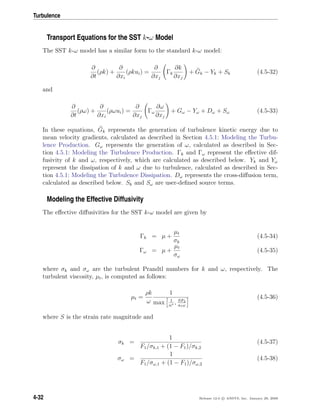
![Turbulence
Although Equation 4.9-28 is solved globally throughout the flow domain, the values of k
obtained are used only for boundary conditions. In every other case, k is obtained from
Equation 4.9-27. This is a minor point, however, since the values of k obtained with
either method should be very similar.
4.9.7 Modeling the Dissipation Rate
The dissipation tensor, ij, is modeled as
ij =
2
3
δij(ρ + YM ) (4.9-29)
where YM = 2ρ M2
t is an additional “dilatation dissipation” term according to the model
by Sarkar [300]. The turbulent Mach number in this term is defined as
Mt =
k
a2
(4.9-30)
where a (≡
√
γRT) is the speed of sound. This compressibility modification always takes
effect when the compressible form of the ideal gas law is used.
The scalar dissipation rate, , is computed with a model transport equation similar to
that used in the standard k- model:
∂
∂t
(ρ ) +
∂
∂xi
(ρ ui) =
∂
∂xj
µ +
µt
σ
∂
∂xj
C 1
1
2
[Pii + C 3Gii]
k
− C 2ρ
2
k
+ S (4.9-31)
where σ = 1.0, C 1 = 1.44, C 2 = 1.92, C 3 is evaluated as a function of the local flow
direction relative to the gravitational vector, as described in Section 4.4.5: Effects of
Buoyancy on Turbulence in the k- Models, and S is a user-defined source term.
In the case when the Reynolds Stress model is coupled with the omega equation, the
dissipation tensor ij is modeled as
ij = 2/3δijρβ∗
RSM kω (4.9-32)
Where β∗
RSM is defined in Section 4.9.4: Modeling the Pressure-Strain Term and the
specific dissipation rate ω is computed in the same way as for the standard k − ω model,
using Equation 4.5-2.
4-56 Release 12.0 c ANSYS, Inc. January 29, 2009](https://image.slidesharecdn.com/flth-130501182911-phpapp02/85/Flth-156-320.jpg)
![Turbulence
where uτ is the friction velocity defined by uτ ≡ τw/ρ, where τw is the wall-shear stress.
When this option is chosen, the k transport equation is not solved.
When using enhanced wall treatments as the near-wall treatment, ANSYS FLUENT ap-
plies zero flux wall boundary conditions to the Reynolds stress equations.
4.9.10 Convective Heat and Mass Transfer Modeling
With the Reynolds stress model in ANSYS FLUENT, turbulent heat transport is modeled
using the concept of Reynolds’ analogy to turbulent momentum transfer. The “modeled”
energy equation is thus given by the following:
∂
∂t
(ρE) +
∂
∂xi
[ui(ρE + p)] =
∂
∂xj
k +
cpµt
Prt
∂T
∂xj
+ ui(τij)eff + Sh (4.9-36)
where E is the total energy and (τij)eff is the deviatoric stress tensor, defined as
(τij)eff = µeff
∂uj
∂xi
+
∂ui
∂xj
−
2
3
µeff
∂uk
∂xk
δij
The term involving (τij)eff represents the viscous heating, and is always computed in the
density-based solvers. It is not computed by default in the pressure-based solver, but it
can be enabled in the Viscous Model dialog box. The default value of the turbulent
Prandtl number is 0.85. You can change the value of Prt in the Viscous Model dialog
box.
Turbulent mass transfer is treated similarly, with a default turbulent Schmidt number of
0.7. This default value can be changed in the Viscous Model dialog box.
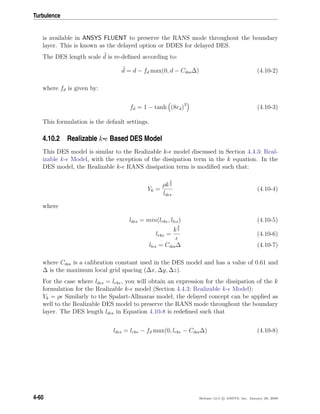
4.10 Detached Eddy Simulation (DES)
This section describes the theory behind the Detached Eddy Simulation (DES) model.
Information is presented in the following sections:
• Section 4.10.1: Spalart-Allmaras Based DES Model
• Section 4.10.2: Realizable k- Based DES Model
• Section 4.10.3: SST k-ω Based DES Model
For details about using the model in ANSYS FLUENT, see Chapter 12: Modeling Turbulence
and Section 12.11: Setting Up the Detached Eddy Simulation Model in the separate User’s
Guide.
4-58 Release 12.0 c ANSYS, Inc. January 29, 2009](https://image.slidesharecdn.com/flth-130501182911-phpapp02/85/Flth-158-320.jpg)
![4.10 Detached Eddy Simulation (DES)
Overview
ANSYS FLUENT offers three different models for the detached eddy simulation: the
Spalart-Allmaras model, the realizable k- model, and the SST k-ω model.
In the DES approach, the unsteady RANS models are employed in the boundary layer,
while the LES treatment is applied to the separated regions. The LES region is normally
associated with the core turbulent region where large unsteady turbulence scales play a
dominant role. In this region, the DES models recover LES-like subgrid models. In the
near-wall region, the respective RANS models are recovered.
DES models have been specifically designed to address high Reynolds number wall
bounded flows, where the cost of a near-wall resolving Large Eddy Simulation would
be prohibitive. The difference with the LES model is that it relies only on the required
resolution in the boundary layers. The application of DES, however, may still require
significant CPU resources and therefore, as a general guideline, it is recommended that
the conventional turbulence models employing the Reynolds-averaged approach be used
for practical calculations.
The DES models, often referred to as the hybrid LES/RANS models combine RANS
modeling with LES for applications such as high-Re external aerodynamics simulations.
In ANSYS FLUENT, the DES model is based on the one-equation Spalart-Allmaras model,
the realizable k- model, and the SST k-ω model. The computational costs, when using
the DES models, is less than LES computational costs, but greater than RANS.
4.10.1 Spalart-Allmaras Based DES Model
The standard Spalart-Allmaras model uses the distance to the closest wall as the defini-
tion for the length scale d, which plays a major role in determining the level of production
and destruction of turbulent viscosity (Equations 4.3-6, 4.3-12, and 4.3-15). The DES
model, as proposed by Shur et al. [314] replaces d everywhere with a new length scale d,
defined as
d = min(d, Cdes∆) (4.10-1)
where the grid spacing, ∆, is based on the largest grid space in the x, y, or z directions
forming the computational cell. The empirical constant Cdes has a value of 0.65.
For a typical RANS grid with a high aspect ratio in the boundary layer, and where the
wall-parallel grid spacing usually exceeds δ, where δ is the size of the boundary layer,
Equation 4.10-1 will ensure that the DES model is in the RANS mode for the entire
boundary layer. However, in case of an ambiguous grid definition, where ∆ << δ, the
DES limiter can activate the LES mode inside the boundary layer, where the grid is not
fine enough to sustain resolved turbulence. Therefore, a new formulation [332] of DES
Release 12.0 c ANSYS, Inc. January 29, 2009 4-59](https://image.slidesharecdn.com/flth-130501182911-phpapp02/85/Flth-159-320.jpg)
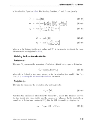
![4.11 Large Eddy Simulation (LES) Model
4.10.3 SST k-ω Based DES Model
The dissipation term of the turbulent kinetic energy (see Section 4.5.1: Modeling the Tur-
bulence Dissipation) is modified for the DES turbulence model as described in Menter’s
work [225] such that
Yk = ρβ∗
kωFDES (4.10-9)
where FDES is expressed as
FDES = max
Lt
Cdes∆
, 1 (4.10-10)
where Cdes is a calibration constant used in the DES model and has a value of 0.61, ∆ is
the maximum local grid spacing (∆x, ∆y, ∆z).
The turbulent length scale is the parameter that defines this RANS model:
Lt =
√
k
β∗ω
(4.10-11)
The DES-SST model also offers the option to “protect” the boundary layer from the
limiter (delayed option). This is achieved with the help of the zonal formulation of the
SST model. FDES is modified according to
FDES = max
Lt
Cdes∆
(1 − FSST ), 1 (4.10-12)
with FSST = 0, F1, F2, where F1 and F2 are the blending functions of the SST model.
The default settings use F2.
4.11 Large Eddy Simulation (LES) Model
This section describes the theory behind the Large Eddy Simulation (LES) model. In-
formation is presented in the following sections:
• Section 4.11.1: Overview
• Section 4.11.2: Filtered Navier-Stokes Equations
• Section 4.11.3: Subgrid-Scale Models
• Section 4.11.4: Inlet Boundary Conditions for the LES Model
Release 12.0 c ANSYS, Inc. January 29, 2009 4-61](https://image.slidesharecdn.com/flth-130501182911-phpapp02/85/Flth-161-320.jpg)
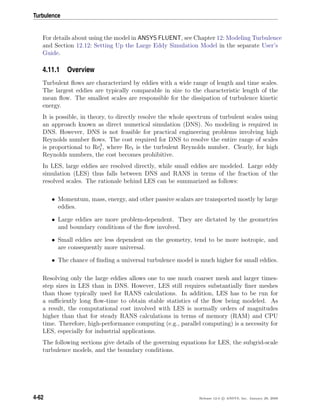
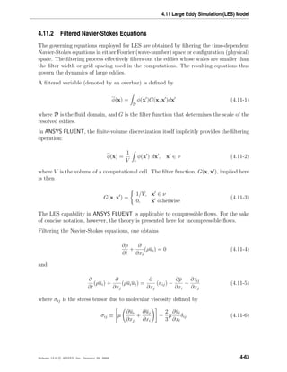
![Turbulence
and τij is the subgrid-scale stress defined by
τij ≡ ρuiuj − ρuiuj (4.11-7)
4.11.3 Subgrid-Scale Models
The subgrid-scale stresses resulting from the filtering operation are unknown, and require
modeling. The subgrid-scale turbulence models in ANSYS FLUENT employ the Boussi-
nesq hypothesis [130] as in the RANS models, computing subgrid-scale turbulent stresses
from
τij −
1
3
τkkδij = −2µtSij (4.11-8)
where µt is the subgrid-scale turbulent viscosity. The isotropic part of the subgrid-scale
stresses τkk is not modeled, but added to the filtered static pressure term. Sij is the
rate-of-strain tensor for the resolved scale defined by
Sij ≡
1
2
∂ui
∂xj
+
∂uj
∂xi
(4.11-9)
For compressible flows, it is convenient to introduce the density-weighted (or Favre)
filtering operator:
φ =
ρφ
ρ
(4.11-10)
The Favre Filtered Navier-Stokes equation takes the same form as Equation 4.11-5. The
compressible form of the subgrid stress tensor is defined as:
τij = ρuiuj − ρuiuj (4.11-11)
This term is split into its isotropic and deviatoric parts
τij = τij −
1
3
τkkδij
deviatoric
+
1
3
τkkδij
isotropic
(4.11-12)
The deviatoric part of the subgrid-scale stress tensor is modeled using the compressible
form of the Smagorinsky model:
τij −
1
3
τkkδij = 2µt(Sij −
1
3
§kkδij) (4.11-13)
4-64 Release 12.0 c ANSYS, Inc. January 29, 2009](https://image.slidesharecdn.com/flth-130501182911-phpapp02/85/Flth-164-320.jpg)
![4.11 Large Eddy Simulation (LES) Model
As for incompressible flows, the term involving τkk can be added to the filtered pressure
or simply neglected [89]. Indeed, this term can be re-written as τkk = γM2
sgsp where
Msgs is the subgrid Mach number. This subgrid Mach number can be expected to be
small when the turbulent Mach number of the flow is small.
ANSYS FLUENT offers four models for µt: the Smagorinsky-Lilly model, the dynamic
Smagorinsky-Lilly model, the WALE model, and the dynamic kinetic energy subgrid-
scale model.
The subgrid-scale turbulent flux of a scalar, φ, is modeled using s subgrid-scale turbulent
Prandtl number by
qj = −
µt
σt
∂φ
∂xj
(4.11-14)
where qj is the subgrid-scale flux.
In the dynamic models, the subgrid-scale turbulent Prandtl number or Schmidt number
is obtained by applying the dynamic procedure originally proposed by Germano [106] to
the subgrid-scale flux.
Smagorinsky-Lilly Model
This simple model was first proposed by Smagorinsky [320]. In the Smagorinsky-Lilly
model, the eddy-viscosity is modeled by
µt = ρL2
s S (4.11-15)
where Ls is the mixing length for subgrid scales and S ≡ 2SijSij. In ANSYS FLUENT,
Ls is computed using
Ls = min (κd, Cs∆) (4.11-16)
where κ is the von K´arm´an constant, d is the distance to the closest wall, Cs is the
Smagorinsky constant, and ∆ is the local grid scale. In ANSYS FLUENT, ∆ is computed
according to the volume of the computational cell using
∆ = V 1/3
(4.11-17)
Lilly derived a value of 0.17 for Cs for homogeneous isotropic turbulence in the inertial
subrange. However, this value was found to cause excessive damping of large-scale fluc-
tuations in the presence of mean shear and in transitional flows as near solid boundary,
and has to be reduced in such regions. In short, Cs is not a universal constant, which
is the most serious shortcoming of this simple model. Nonetheless, a Cs value of around
Release 12.0 c ANSYS, Inc. January 29, 2009 4-65](https://image.slidesharecdn.com/flth-130501182911-phpapp02/85/Flth-165-320.jpg)
![Turbulence
0.1 has been found to yield the best results for a wide range of flows, and is the default
value in ANSYS FLUENT.
Dynamic Smagorinsky-Lilly Model
Germano et al. [106] and subsequently Lilly [197] conceived a procedure in which the
Smagorinsky model constant, Cs, is dynamically computed based on the information
provided by the resolved scales of motion. The dynamic procedure thus obviates the
need for users to specify the model constant Cs in advance.
The concept of the dynamic procedure is to apply a second filter (called the test filter) to
the equations of motion. The new filter width ˆ∆ is equal to twice the grid filter width ∆.
Both filters produce a resolved flow field. The difference between the two resolved fields
is the contribution of the small scales whose size is in between the grid filter and the test
filter. The information related to these scales is used to compute the model constant. In
ANSYS FLUENT, the variable density formulation of the model is considered as explained
below.
At the test filtered field level, the SGS stress tensor can be expressed as:
Tij = ρuiuj − (ρui ρuj/ρ) (4.11-18)
Both Tij and τij are modeled in the same way with the Smagorinsky-Lilly model, assuming
scale similarity:
τij = −2Cρ∆2
S|(Sij −
1
3
Skkδij) (4.11-19)
Tij = −2Cρ∆2
|S|(Sij −
1
3
Skkδij) (4.11-20)
In Equation 4.11-19 and Equation 4.11-20, the coefficient C is asumed to be the same
and independent of the filtering process (note that per Equation 4.11-25, C = C2
s ). The
grid filtered SGS and the test-filtered SGS are related by the Germano identity [106] such
that:
Lij = Tij − τij = ρuiuj −
1
ρ
(ρuiρuj) (4.11-21)
Where Lij is computable from the resolved large eddy field. Substituting the grid-filter
Smagorinsky-Lilly model and Equation 4.11-20 into Equation 4.11-21, the following ex-
pressions can be derived to solve for C with the contraction obtained from the least
square analysis of Lilly (1992).
4-66 Release 12.0 c ANSYS, Inc. January 29, 2009](https://image.slidesharecdn.com/flth-130501182911-phpapp02/85/Flth-166-320.jpg)
![4.11 Large Eddy Simulation (LES) Model
C =
(Lij − Lkkδij/3)
MijMij
(4.11-22)
With
Mij = −2 ∆2
ρ |S|Sij − ∆2
ρ |S|Sij (4.11-23)
More details of the model implementation in ANSYS FLUENT and its validation can be
found in [165].
The Cs =
√
C obtained using the dynamic Smagorinsky-Lilly model varies in time and
space over a fairly wide range. To avoid numerical instability, both the numerator and
the denominator in Equation 4.11-22 are locally averaged (or filtered) using the test-filter.
In ANSYS FLUENT, Cs is also clipped at zero and 0.23 by default.
Wall-Adapting Local Eddy-Viscosity (WALE) Model
In the WALE model [248], the eddy viscosity is modeled by
µt = ρL2
s
(Sd
ijSd
ij)3/2
(SijSij)5/2 + (Sd
ijSd
ij)5/4
(4.11-24)
where Ls and Sd
ij in the WALE model are defined, respectively, as
Ls = min κd, CwV 1/3
(4.11-25)
Sd
ij =
1
2
g2
ij + g2
ji −
1
3
δijg2
kk , gij =
∂ui
∂xj
(4.11-26)
In ANSYS FLUENT, the default value of the WALE constant, Cw, is 0.325 and has been
found to yield satisfactory results for a wide range of flow. The rest of the notation is the
same as for the Smagorinsky-Lilly model. With this spatial operator, the WALE model
is designed to return the correct wall asymptotic (y3
) behavior for wall bounded flows.
Dynamic Kinetic Energy Subgrid-Scale Model
The original and dynamic Smagorinsky-Lilly models, discussed previously, are essentially
algebraic models in which subgrid-scale stresses are parameterized using the resolved ve-
locity scales. The underlying assumption is the local equilibrium between the transferred
energy through the grid-filter scale and the dissipation of kinetic energy at small sub-
grid scales. The subgrid-scale turbulence can be better modeled by accounting for the
transport of the subgrid-scale turbulence kinetic energy.
Release 12.0 c ANSYS, Inc. January 29, 2009 4-67](https://image.slidesharecdn.com/flth-130501182911-phpapp02/85/Flth-167-320.jpg)
![Turbulence
The dynamic subgrid-scale kinetic energy model in ANSYS FLUENT replicates the model
proposed by Kim and Menon [168].
The subgrid-scale kinetic energy is defined as
ksgs =
1
2
u2
k − u2
k (4.11-27)
which is obtained by contracting the subgrid-scale stress in Equation 4.11-7.
The subgrid-scale eddy viscosity, µt, is computed using ksgs as
µt = Ckk1/2
sgs ∆f (4.11-28)
where ∆f is the filter-size computed from ∆f ≡ V 1/3
.
The subgrid-scale stress can then be written as
τij −
2
3
ksgsδij = −2Ckk1/2
sgs ∆f Sij (4.11-29)
ksgs is obtained by solving its transport equation
∂ksgs
∂t
+
∂ujksgs
∂xj
= −τij
∂ui
∂xj
− Cε
k3/2
sgs
∆f
+
∂
∂xj
µt
σk
∂ksgs
∂xj
(4.11-30)
In the above equations, the model constants, Ck and Cε, are determined dynamically [168].
σk is hardwired to 1.0. The details of the implementation of this model in ANSYS FLU-
ENT and its validation is given by Kim [165].
4.11.4 Inlet Boundary Conditions for the LES Model
This section describes the three algorithms available in ANSYS FLUENT to model the
fluctuating velocity at velocity inlet boundaries or pressure inlet boundaries.
No Perturbations
The stochastic components of the flow at the velocity-specified inlet boundaries are ne-
glected if the No Perturbations option is used. In such cases, individual instantaneous
velocity components are simply set equal to their mean velocity counterparts. This op-
tion is suitable only when the level of turbulence at the inflow boundaries is negligible or
does not play a major role in the accuracy of the overall solution.
4-68 Release 12.0 c ANSYS, Inc. January 29, 2009](https://image.slidesharecdn.com/flth-130501182911-phpapp02/85/Flth-168-320.jpg)
![4.11 Large Eddy Simulation (LES) Model
Vortex Method
To generate a time-dependent inlet condition, a random 2D vortex method is considered.
With this approach, a perturbation is added on a specified mean velocity profile via a
fluctuating vorticity field (i.e. two-dimensional in the plane normal to the streamwise
direction). The vortex method is based on the Lagrangian form of the 2D evolution
equation of the vorticity and the Biot-Savart law. A particle discretization is used to
solve this equation. These particles, or “vortex points” are convected randomly and
carry information about the vorticity field. If N is the number of vortex points and A
is the area of the inlet section, the amount of vorticity carried by a given particle i is
represented by the circulation Γi and an assumed spatial distribution η:
Γi(x, y) = 4
πAk(x, y)
3N[2 ln(3) − 3 ln(2)]
(4.11-31)
η(x) =
1
2πσ2
2e−|x|2/2σ2
− 1 2e−|x|2/2σ2
(4.11-32)
where k is the turbulence kinetic energy. The parameter σ provides control over the size
of a vortex particle. The resulting discretization for the velocity field is given by
u(x) =
1
2π
N
i=1
Γi
((xi − x) × z)(1 − e|x−x |2/2σ2
)
|x − xi|2
(4.11-33)
Where z is the unit vector in the streamwise direction. Originally [311], the size of
the vortex was fixed by an ad hoc value of σ. To make the vortex method generally
applicable, a local vortex size is specified through a turbulent mixing length hypothesis. σ
is calculated from a known profile of mean turbulence kinetic energy and mean dissipation
rate at the inlet according to the following:
σ =
ck3/2
2
(4.11-34)
where c = 0.16. To ensure that the vortex will always belong to resolved scales, the
minimum value of σ in Equation 4.11-34 is bounded by the local grid size. The sign
of the circulation of each vortex is changed randomly each characteristic time scale τ.
In the general implementation of the vortex method, this time scale represents the time
necessary for a 2D vortex convected by the bulk velocity in the boundary normal direction
to travel along n times its mean characteristic 2D size (σm), where n is fixed equal to
100 from numerical testing. The vortex method considers only velocity fluctuations in
the plane normal to the streamwise direction.
Release 12.0 c ANSYS, Inc. January 29, 2009 4-69](https://image.slidesharecdn.com/flth-130501182911-phpapp02/85/Flth-169-320.jpg)
![Turbulence
In ANSYS FLUENT however, a simplified linear kinematic model (LKM) for the stream-
wise velocity fluctuations is used [219]. It is derived from a linear model that mimics
the influence of the two-dimensional vortex in the streamwise mean velocity field. If the
mean streamwise velocity U is considered as a passive scalar, the fluctuation u resulting
from the transport of U by the planar fluctuating velocity field v is modeled by
u = −v · g (4.11-35)
where g is the unit vector aligned with the mean velocity gradient U. When this mean
velocity gradient is equal to zero, a random perturbation can be considered instead.
Since the fluctuations are equally distributed among the velocity components, only the
prescribed kinetic energy profile can be fulfilled at the inlet of the domain. Farther
downstream, the correct fluctuation distribution is recovered [219]. However, if the dis-
tribution of the normal fluctuations is known or can be prescribed at the inlet, a rescaling
technique can be applied to the synthetic flow field in order to fulfill the normal statistic
fluctuations < uu >, < vv >, and < ww > as given at the inlet.
With the rescaling procedure, the velocity fluctuations are expressed according to:
u ∗
i = ui
√
< uiui >
2/3k
(4.11-36)
This also results in an improved representation of the turbulent flow field downstream
of the inlet. This rescaling procedure is used only if the Reynolds-Stress Components is
specified as the Reynolds-Stress Specification Method, instead of the default option K or
Turbulence Intensity.
i Since the vortex method theory is based on the modification of the velocity
field normal to the streamwise direction, it is imperative that you create
an inlet plane normal (or as close as possible) to the streamwise velocity
direction.
Spectral Synthesizer
The spectral synthesizer provides an alternative method of generating fluctuating velocity
components. It is based on the random flow generation technique originally proposed
by Kraichnan [171] and modified by Smirnov et al. [321]. In this method, fluctuating
velocity components are computed by synthesizing a divergence-free velocity-vector field
from the summation of Fourier harmonics. In ANSYS FLUENT, the number of Fourier
harmonics is fixed to 100.
4-70 Release 12.0 c ANSYS, Inc. January 29, 2009](https://image.slidesharecdn.com/flth-130501182911-phpapp02/85/Flth-170-320.jpg)
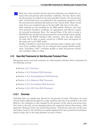
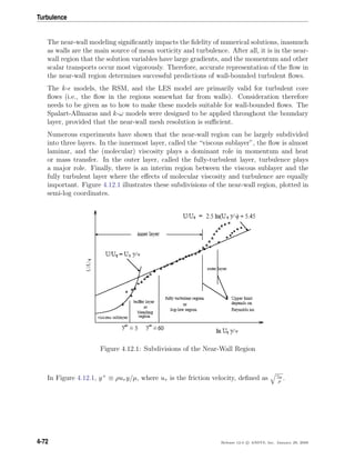
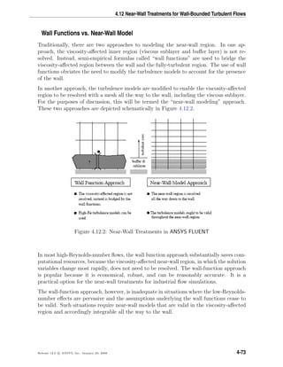
![Turbulence
ANSYS FLUENT provides both the wall-function approach and the near-wall modeling
approach.
Wall Functions
Wall functions are a set of semi-empirical formulas and functions that in effect “bridge”
or “link” the solution variables at the near-wall cells and the corresponding quantities
on the wall. The wall functions comprise
• laws-of-the-wall for the mean velocity and temperature (or other scalars)
• formulae for the near-wall turbulent quantities
Depending on the choice of turbulent model, ANSYS FLUENT offers three to four choices
of wall-function approaches:
• Standard Wall Functions
• Non-Equilibrium Wall Functions
• Enhanced Wall Functions (as a part of EWT)
• User-Defined Wall Functions
4.12.2 Standard Wall Functions
The standard wall functions in ANSYS FLUENT are based on the work of Launder and
Spalding [181], and have been most widely used in industrial flows. They are provided
as a default option in ANSYS FLUENT.
Momentum
The law-of-the-wall for mean velocity yields
U∗
=
1
κ
ln(Ey∗
) (4.12-1)
where
U∗
≡
UP C1/4
µ k
1/2
P
τw/ρ
(4.12-2)
is the dimensionless velocity.
4-74 Release 12.0 c ANSYS, Inc. January 29, 2009](https://image.slidesharecdn.com/flth-130501182911-phpapp02/85/Flth-174-320.jpg)
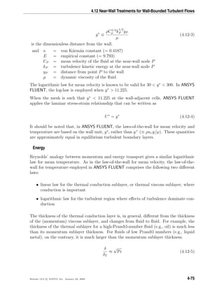
![Turbulence
In highly compressible flows, the temperature distribution in the near-wall region can
be significantly different from that of low subsonic flows, due to the heating by viscous
dissipation. In ANSYS FLUENT, the temperature wall functions include the contribution
from the viscous heating [357].
The law-of-the-wall implemented in ANSYS FLUENT has the following composite form:
T∗
≡
(Tw − TP ) ρcpk
1/2
P
˙q
=
Pr y∗
+ 1
2
ρPr
C
1/4
µ k
1/2
P
˙q
U2
P (y∗
< y∗
T )
Prt
1
κ
ln(Ey∗
) + P +
1
2
ρ
C
1/4
µ k
1/2
P
˙q
{PrtU2
P + (Pr − Prt)U2
c } (y∗
> y∗
T )
(4.12-6)
where P is computed by using the formula given by Jayatilleke [150]:
P = 9.24
Pr
Prt
3/4
− 1 1 + 0.28e−0.007Pr/Prt
(4.12-7)
and
kP = turbulent kinetic energy at the first near-wall node P
ρ = density of fluid
cp = specific heat of fluid
˙q = wall heat flux
TP = temperature at the first near-wall node P
Tw = temperature at the wall
Pr = molecular Prandtl number (µcp/kf )
Prt = turbulent Prandtl number (0.85 at the wall)
A = Van Driest constant (= 26)
Uc = mean velocity magnitude at y∗
= y∗
T
Note that, for the pressure-based solver, the terms
1
2
ρPr
C1/4
µ k
1/2
P
˙q
U2
P
and
1
2
ρ
C1/4
µ k
1/2
P
˙q
PrtU2
P + (Pr − Prt)U2
c
will be included in Equation 4.12-6 only for compressible flow calculations.
The non-dimensional thermal sublayer thickness, y∗
T , in Equation 4.12-6 is computed as
the y∗
value at which the linear law and the logarithmic law intersect, given the molecular
Prandtl number of the fluid being modeled.
4-76 Release 12.0 c ANSYS, Inc. January 29, 2009](https://image.slidesharecdn.com/flth-130501182911-phpapp02/85/Flth-176-320.jpg)
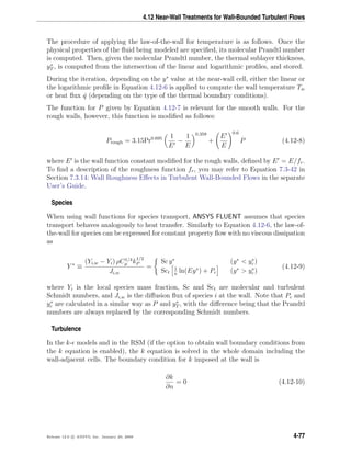
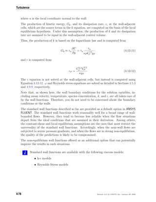
![4.12 Near-Wall Treatments for Wall-Bounded Turbulent Flows
Scalable Wall Functions
The purpose of scalable wall functions is to force the usage of the log law in conjunction
with the standard wall functions approach. This is achieved by introducing a limiter in
the y* calculations such that
y∗ = MAX(y∗, y∗limit) (4.12-13)
where y∗limit = 11.225. The use of Equation 4.12-13 in the context of the scalable wall
functions concept is straightforward, i.e. the y* formulation used for any standard wall
function formula is replaced by y∗.
Scalable wall functions can be enabled only when the standard wall functions are used
and only via the following text command:
define/models/viscous/near-wall-treatment/scalable-wall-functions?
4.12.3 Non-Equilibrium Wall Functions
In addition to the standard wall function described above (which is the default near-wall
treatment) a two-layer-based, non-equilibrium wall function [166] is also available. The
key elements in the non-equilibrium wall functions are as follows:
• Launder and Spalding’s log-law for mean velocity is sensitized to pressure-gradient
effects.
• The two-layer-based concept is adopted to compute the budget of turbulence kinetic
energy (Gk, ) in the wall-neighboring cells.
The law-of-the-wall for mean temperature or species mass fraction remains the same as
in the standard wall functions described above.
The log-law for mean velocity sensitized to the pressure gradients is
UC1/4
µ k1/2
τw/ρ
=
1
κ
ln E
ρC1/4
µ k1/2
y
µ
(4.12-14)
where
U = U −
1
2
dp
dx
yv
ρκ
√
k
ln
y
yv
+
y − yv
ρκ
√
k
+
y2
v
µ
(4.12-15)
and yv is the physical viscous sublayer thickness, and is computed from
Release 12.0 c ANSYS, Inc. January 29, 2009 4-79](https://image.slidesharecdn.com/flth-130501182911-phpapp02/85/Flth-179-320.jpg)
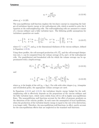
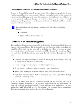
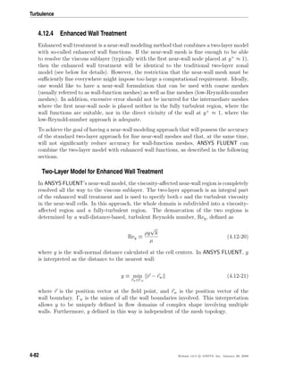
![4.12 Near-Wall Treatments for Wall-Bounded Turbulent Flows
In the fully turbulent region (Rey > Re∗
y; Re∗
y = 200), the k- models or the RSM
(described in Sections 4.4 and 4.9) are employed.
In the viscosity-affected near-wall region (Rey < Re∗
y), the one-equation model of Wolf-
stein [382] is employed. In the one-equation model, the momentum equations and the
k equation are retained as described in Sections 4.4 and 4.9. However, the turbulent
viscosity, µt, is computed from
µt,2layer = ρ Cµ µ
√
k (4.12-22)
where the length scale that appears in Equation 4.12-22 is computed from [51]
µ = yC ∗
1 − e−Rey/Aµ
(4.12-23)
The two-layer formulation for turbulent viscosity described above is used as a part of the
enhanced wall treatment, in which the two-layer definition is smoothly blended with the
high-Reynolds-number µt definition from the outer region, as proposed by Jongen [153]:
µt,enh = λ µt + (1 − λ )µt,2layer (4.12-24)
where µt is the high-Reynolds-number definition as described in Section 4.4: Standard,
RNG, and Realizable k- Models or 4.9 for the k- models or the RSM. A blending
function, λ , is defined in such a way that it is equal to unity away from walls and is zero
in the vicinity of the walls. The blending function has the following form:
λ =
1
2
1 + tanh
Rey − Re∗
y
A
(4.12-25)
The constant A determines the width of the blending function. By defining a width such
that the value of λ will be within 1% of its far-field value given a variation of ∆Rey, the
result is
A =
|∆Rey|
artanh(0.98)
(4.12-26)
Typically, ∆Rey would be assigned a value that is between 5% and 20% of Re∗
y. The
main purpose of the blending function λ is to prevent solution convergence from being
impeded when the value of µt obtained in the outer layer does not match with the value
of µt returned by the Wolfstein model at the edge of the viscosity-affected region.
Release 12.0 c ANSYS, Inc. January 29, 2009 4-83](https://image.slidesharecdn.com/flth-130501182911-phpapp02/85/Flth-183-320.jpg)
![Turbulence
The field in the viscosity-affected region is computed from
=
k3/2
(4.12-27)
The length scales that appear in Equation 4.12-27 are computed from Chen and Patel [51]:
= yC ∗
1 − e−Rey/A
(4.12-28)
If the whole flow domain is inside the viscosity-affected region (Rey < 200), is not
obtained by solving the transport equation; it is instead obtained algebraically from
Equation 4.12-27. ANSYS FLUENT uses a procedure for the blending of that is similar
to the µt-blending in order to ensure a smooth transition between the algebraically-
specified in the inner region and the obtained from solution of the transport equation
in the outer region.
The constants in Equations 4.12-23 and 4.12-28, are taken from [51] and are as follows:
C ∗
= κC−3/4
µ , Aµ = 70, A = 2C ∗
(4.12-29)
Enhanced Wall Functions
To have a method that can extend its applicability throughout the near-wall region
(i.e., viscous sublayer, buffer region, and fully-turbulent outer region) it is necessary to
formulate the law-of-the wall as a single wall law for the entire wall region. ANSYS
FLUENT achieves this by blending the linear (laminar) and logarithmic (turbulent) laws-
of-the-wall using a function suggested by Kader [155]:
u+
= eΓ
u+
lam + e
1
Γ u+
turb (4.12-30)
where the blending function is given by:
Γ = −
a(y+
)4
1 + by+
(4.12-31)
where a = 0.01 and b = 5.
Similarly, the general equation for the derivative du+
dy+ is
du+
dy+
= eΓ du+
lam
dy+
+ e
1
Γ
du+
turb
dy+
(4.12-32)
4-84 Release 12.0 c ANSYS, Inc. January 29, 2009](https://image.slidesharecdn.com/flth-130501182911-phpapp02/85/Flth-184-320.jpg)
![4.12 Near-Wall Treatments for Wall-Bounded Turbulent Flows
This approach allows the fully turbulent law to be easily modified and extended to take
into account other effects such as pressure gradients or variable properties. This formula
also guarantees the correct asymptotic behavior for large and small values of y+
and
reasonable representation of velocity profiles in the cases where y+
falls inside the wall
buffer region (3 < y+
< 10).
The enhanced wall functions were developed by smoothly blending an enhanced turbulent
wall law with the laminar wall law. The enhanced turbulent law-of-the-wall for compress-
ible flow with heat transfer and pressure gradients has been derived by combining the
approaches of White and Cristoph [378] and Huang et al. [134]:
du+
turb
dy+
=
1
κy+
S (1 − βu+
− γ(u+
)2
)
1/2
(4.12-33)
where
S =
1 + αy+
for y+
< y+
s
1 + αy+
s for y+
≥ y+
s
(4.12-34)
and
α ≡
νw
τwu∗
dp
dx
=
µ
ρ2(u∗)3
dp
dx
(4.12-35)
β ≡
σtqwu∗
cpτwTw
=
σtqw
ρcpu∗Tw
(4.12-36)
γ ≡
σt(u∗
)2
2cpTw
(4.12-37)
where y+
s is the location at which the log-law slope is fixed. By default, y+
s = 60. The
coefficient α in Equation 4.12-33 represents the influences of pressure gradients while
the coefficients β and γ represent the thermal effects. Equation 4.12-33 is an ordinary
differential equation and ANSYS FLUENT will provide an appropriate analytical solution.
If α, β, and γ all equal 0, an analytical solution would lead to the classical turbulent
logarithmic law-of-the-wall.
The laminar law-of-the-wall is determined from the following expression:
du+
lam
dy+
= 1 + αy+
(4.12-38)
Release 12.0 c ANSYS, Inc. January 29, 2009 4-85](https://image.slidesharecdn.com/flth-130501182911-phpapp02/85/Flth-185-320.jpg)
![Turbulence
Note that the above expression only includes effects of pressure gradients through α,
while the effects of variable properties due to heat transfer and compressibility on the
laminar wall law are neglected. These effects are neglected because they are thought to be
of minor importance when they occur close to the wall. Integration of Equation 4.12-38
results in
u+
lam = y+
1 +
α
2
y+
(4.12-39)
Enhanced thermal wall functions follow the same approach developed for the profile of
u+
. The unified wall thermal formulation blends the laminar and logarithmic profiles
according to the method of Kader [155]:
T+
≡
(Tw − TP ) ρcpuT
˙q
= eΓ
T+
lam + e
1
Γ T+
turb (4.12-40)
where the notation for TP and ˙q is the same as for standard thermal wall functions (see
Equation 4.12-6). Furthermore, the blending factor Γ is defined as
Γ = −
a(Pr y+
)4
1 + bPr3
y+
(4.12-41)
where Pr is the molecular Prandtl number, and the coefficients a and b are defined as in
Equation 4.12-31.
Apart from the formulation for T+
in Equation 4.12-40, the enhanced thermal wall func-
tions follow the same logic as for standard thermal wall functions (see Section 4.12.2: Energy),
resulting in the following definition for turbulent and laminar thermal wall functions:
T+
lam = Pr u+
lam +
ρu∗
2 ˙q
u2
(4.12-42)
T+
turb = Prt u+
turb + P +
ρu∗
2 ˙q
u2
−
Pr
Prt
− 1 (u+
c )2
(u∗)2
(4.12-43)
where the quantity u+
c is the value of u+
at the fictitious “crossover” between the laminar
and turbulent region. The function P is defined in the same way as for the standard wall
functions.
A similar procedure is also used for species wall functions when the enhanced wall treat-
ment is used. In this case, the Prandtl numbers in Equations 4.12-42 and 4.12-43 are
replaced by adequate Schmidt numbers. See Section 4.12.2: Species for details about the
species wall functions.
4-86 Release 12.0 c ANSYS, Inc. January 29, 2009](https://image.slidesharecdn.com/flth-130501182911-phpapp02/85/Flth-186-320.jpg)
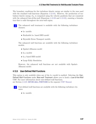
![Turbulence
4.12.6 LES Near-Wall Treatment
When the mesh is fine enough to resolve the laminar sublayer, the wall shear stress is
obtained from the laminar stress-strain relationship:
u
uτ
=
ρuτ y
µ
(4.12-44)
If the mesh is too coarse to resolve the laminar sublayer, it is assumed that the centroid
of the wall-adjacent cell falls within the logarithmic region of the boundary layer, and
the law-of-the-wall is employed:
u
uτ
=
1
κ
ln E
ρuτ y
µ
(4.12-45)
where κ is the von K´arm´an constant and E = 9.793. If the mesh is such that the first
near-wall point is within the buffer region, then two above laws are blended in accordance
with the Equation 4.12-30.
For the LES simulations in ANSYS FLUENT, there is an alternative near-wall approach
based on the work of Werner and Wengle [375], who proposed an analytical integration
of the power-law near-wall velocity distribution resulting in the following expressions for
the wall shear stress:
|τw| =
2µ|up|
∆z
for |up| ≤ µ
2ρ∆z
A
2
1−B
ρ 1−B
2
A
1+B
1−B
µ
ρ∆z
1+B
+ 1+B
A
µ
ρ∆z
B
|up|
2
1+B
for |up| > µ
2ρ∆z
A
2
1−B
(4.12-46)
where up is the wall-parallel velocity, A = 8.3, B = 1/7 are the constants, and ∆z is the
near-wall control volume length scale.
The Werner-Wengle wall functions can be enabled using the define/models/viscous/
near-wall-treatment/werner-wengle-wall-fn? text command.
4-88 Release 12.0 c ANSYS, Inc. January 29, 2009](https://image.slidesharecdn.com/flth-130501182911-phpapp02/85/Flth-188-320.jpg)
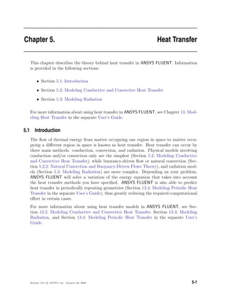
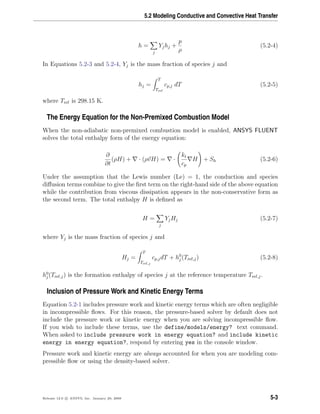
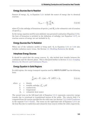
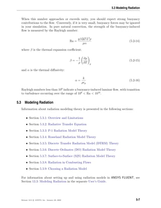
![Heat Transfer
5.3.1 Overview and Limitations
ANSYS FLUENT provides five radiation models which allow you to include radiation,
with or without a participating medium, in your heat transfer simulations.
Heating or cooling of surfaces due to radiation and/or heat sources or sinks due to
radiation within the fluid phase can be included in your model using one of the following
radiation models.
• Discrete Transfer Radiation Model (DTRM) [47, 312]
• P-1 Radiation Model [52, 315]
• Rosseland Radiation Model [315]
• Surface-to-Surface (S2S) Radiation Model [315]
• Discrete Ordinates (DO) Radiation Model [56, 282]
In addition to these radiation models, ANSYS FLUENT also provides a solar load model
that allows you to include the effects of solar radiation in your simulation.
Typical applications well suited for simulation using radiative heat transfer include the
following:
• radiative heat transfer from flames
• surface-to-surface radiant heating or cooling
• coupled radiation, convection, and/or conduction heat transfer
• radiation through windows in HVAC applications, and cabin heat transfer analysis
in automotive applications
• radiation in glass processing, glass fiber drawing, and ceramic processing
You should include radiative heat transfer in your simulation when the radiant heat flux,
Qrad = σ(T4
max − T4
min), is large compared to the heat transfer rate due to convection
or conduction. Typically this will occur at high temperatures where the fourth-order
dependence of the radiative heat flux on temperature implies that radiation will dominate.
5-8 Release 12.0 c ANSYS, Inc. January 29, 2009](https://image.slidesharecdn.com/flth-130501182911-phpapp02/85/Flth-196-320.jpg)
![Heat Transfer
Advantages and Limitations of the Rosseland Model
The Rosseland model has two advantages over the P-1 model. Since it does not solve an
extra transport equation for the incident radiation (as the P-1 model does), the Rosseland
model is faster than the P-1 model and requires less memory.
The Rosseland model can be used only for optically thick media. It is recommended for
use when the optical thickness exceeds 3. Note also that the Rosseland model is not
available when the density-based solver is being used; it is available with the pressure-
based solver, only.
Advantages and Limitations of the DO Model
The DO model spans the entire range of optical thicknesses, and allows you to solve prob-
lems ranging from surface-to-surface radiation to participating radiation in combustion
problems. It also allows the solution of radiation at semi-transparent walls. Computa-
tional cost is moderate for typical angular discretizations, and memory requirements are
modest.
The current implementation is restricted to either gray radiation or non-gray radiation
using a gray-band model. Solving a problem with a fine angular discretization may be
CPU-intensive.
The non-gray implementation in ANSYS FLUENT is intended for use with participating
media with a spectral absorption coefficient aλ that varies in a stepwise fashion across
spectral bands, but varies smoothly within the band. Glass, for example, displays banded
behavior of this type. The current implementation does not model the behavior of gases
such as carbon dioxide or water vapor, which absorb and emit energy at distinct wave
numbers [234]. The modeling of non-gray gas radiation is still an evolving field. However,
some researchers [98] have used gray-band models to model gas behavior by approximat-
ing the absorption coefficients within each band as a constant. The implementation in
ANSYS FLUENT can be used in this fashion if desired.
The non-gray implementation in ANSYS FLUENT is compatible with all the models with
which the gray implementation of the DO model can be used. Thus, it is possible to
include scattering, anisotropy, semi-transparent media, and particulate effects. How-
ever, the non-gray implementation assumes a constant absorption coefficient within each
wavelength band. The weighted-sum-of-gray-gases model (WSGGM) cannot be used to
specify the absorption coefficient in each band. The implementation allows the specifi-
cation of spectral emissivity at walls. The emissivity is assumed to be constant within
each band.
5-10 Release 12.0 c ANSYS, Inc. January 29, 2009](https://image.slidesharecdn.com/flth-130501182911-phpapp02/85/Flth-198-320.jpg)
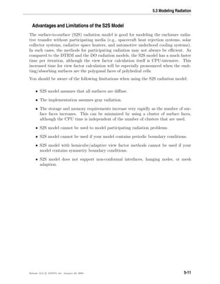
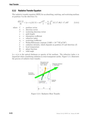
![5.3 Modeling Radiation
The DTRM and the P-1, Rosseland, and DO radiation models require the absorption
coefficient a as input. a and the scattering coefficient σs can be constants, and a can also
be a function of local concentrations of H2O and CO2, path length, and total pressure.
ANSYS FLUENT provides the weighted-sum-of-gray-gases model (WSGGM) for compu-
tation of a variable absorption coefficient. See Section 5.3.8: Radiation in Combusting
Flows for details. The discrete ordinates implementation can model radiation in semi-
transparent media. The refractive index n of the medium must be provided as a part of
the calculation for this type of problem. The Rosseland model also requires you to enter
a refractive index, or use the default value of 1.
5.3.3 P-1 Radiation Model Theory
The P-1 radiation model is the simplest case of the more general P-N model, which is
based on the expansion of the radiation intensity I into an orthogonal series of spherical
harmonics [52, 315]. This section provides details about the equations used in the P-1
model. For information about setting up the model, see Section 13.3.1: Steps in Using
the Radiation Models in the separate User’s Guide.
The P-1 Model Equations
As mentioned above, the P-1 radiation model is the simplest case of the P-N model. If
only four terms in the series are used, the following equation is obtained for the radiation
flux qr:
qr = −
1
3(a + σs) − Cσs
G (5.3-2)
where a is the absorption coefficient, σs is the scattering coefficient, G is the incident
radiation, and C is the linear-anisotropic phase function coefficient, described below.
After introducing the parameter
Γ =
1
(3(a + σs) − Cσs)
(5.3-3)
Equation 5.3-2 simplifies to
qr = −Γ G (5.3-4)
The transport equation for G is
· (Γ G) − aG + 4an2
σT4
= SG (5.3-5)
Release 12.0 c ANSYS, Inc. January 29, 2009 5-13](https://image.slidesharecdn.com/flth-130501182911-phpapp02/85/Flth-201-320.jpg)
![Heat Transfer
Boundary Condition Treatment for the P-1 Model at Walls
To get the boundary condition for the incident radiation equation, the dot product of
the outward normal vector n and Equation 5.3-4 is computed:
qr · n = −Γ G · n (5.3-15)
qr,w = −Γ
∂G
∂n
(5.3-16)
Thus the flux of the incident radiation, G, at a wall is −qr,w. The wall radiative heat
flux is computed using the following boundary condition:
Iw(r, s) = fw(r, s) (5.3-17)
fw(r, s) = w
n2
σT4
w
π
+ ρwI(r, −s) (5.3-18)
where ρw is the wall reflectivity. The Marshak boundary condition is then used to elim-
inate the angular dependence [262]:
2π
0
Iw(r, s) n · s dΩ =
2π
0
fw(r, s) n · s dΩ (5.3-19)
Substituting Equations 5.3-17 and 5.3-18 into Equation 5.3-19 and performing the inte-
grations yields
qr,w = −
4π w
n2σT4
w
π
− (1 − ρw)Gw
2(1 + ρw)
(5.3-20)
If it is assumed that the walls are diffuse gray surfaces, then ρw = 1 − w, and Equa-
tion 5.3-20 becomes
qr,w = −
w
2 (2 − w)
4n2
σT4
w − Gw (5.3-21)
Equation 5.3-21 is used to compute qr,w for the energy equation and for the incident
radiation equation boundary conditions.
5-16 Release 12.0 c ANSYS, Inc. January 29, 2009](https://image.slidesharecdn.com/flth-130501182911-phpapp02/85/Flth-204-320.jpg)
![Heat Transfer
Since the radiative heat flux has the same form as the Fourier conduction law, it is
possible to write
q = qc + qr (5.3-24)
= −(k + kr) T (5.3-25)
kr = 16σΓn2
T3
(5.3-26)
where k is the thermal conductivity and kr is the radiative conductivity. Equation 5.3-24
is used in the energy equation to compute the temperature field.
Anisotropic Scattering
The Rosseland model allows for anisotropic scattering, using the same phase function
(Equation 5.3-7) described for the P-1 model in Section 5.3.3: Anisotropic Scattering.
Boundary Condition Treatment for the Rosseland Model at Walls
Since the diffusion approximation is not valid near walls, it is necessary to use a tem-
perature slip boundary condition. The radiative heat flux at the wall boundary, qr,w, is
defined using the slip coefficient ψ:
qr,w = −
σ T4
w − T4
g
ψ
(5.3-27)
where Tw is the wall temperature, Tg is the temperature of the gas at the wall, and the
slip coefficient ψ is approximated by a curve fit to the plot given in [315]:
ψ =
1/2 Nw < 0.01
2x3+3x2−12x+7
54
0.01 ≤ Nw ≤ 10
0 Nw > 10
(5.3-28)
where Nw is the conduction to radiation parameter at the wall:
Nw =
k(a + σs)
4σT3
w
(5.3-29)
and x = log10 Nw.
5-18 Release 12.0 c ANSYS, Inc. January 29, 2009](https://image.slidesharecdn.com/flth-130501182911-phpapp02/85/Flth-206-320.jpg)
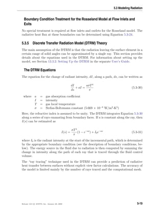
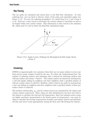
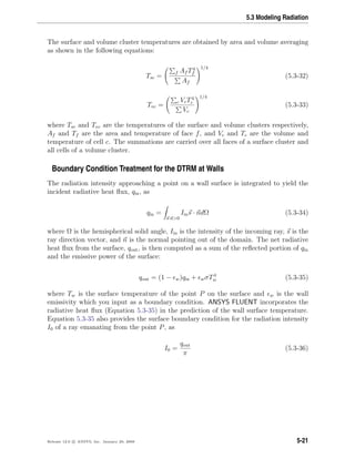
![Heat Transfer
Boundary Condition Treatment for the DTRM at Flow Inlets and Exits
The net radiative heat flux at flow inlets and outlets is computed in the same manner as at
walls, as described above. ANSYS FLUENT assumes that the emissivity of all flow inlets
and outlets is 1.0 (black body absorption) unless you choose to redefine this boundary
treatment.
ANSYS FLUENT includes an option that allows you to use different temperatures for
radiation and convection at inlets and outlets. This can be useful when the temperature
outside the inlet or outlet differs considerably from the temperature in the enclosure. See
Section 13.3.6: Defining Boundary Conditions for Radiation in the separate User’s Guide
for details.
5.3.6 Discrete Ordinates (DO) Radiation Model Theory
The discrete ordinates (DO) radiation model solves the radiative transfer equation (RTE)
for a finite number of discrete solid angles, each associated with a vector direction s fixed
in the global Cartesian system (x, y, z). The fineness of the angular discretization is
controlled by you, analogous to choosing the number of rays for the DTRM. Unlike the
DTRM, however, the DO model does not perform ray tracing. Instead, the DO model
transforms Equation 5.3-1 into a transport equation for radiation intensity in the spatial
coordinates (x, y, z). The DO model solves for as many transport equations as there are
directions s. The solution method is identical to that used for the fluid flow and energy
equations.
Two implementations of the DO model are available in ANSYS FLUENT: uncoupled and
(energy) coupled. The uncoupled implementation is sequential in nature and uses a
conservative variant of the DO model called the finite-volume scheme [56, 282], and its
extension to unstructured meshes [242]. In the uncoupled case, the equations for the
energy and radiation intensities are solved one by one, assuming prevailing values for
other variables.
Alternatively, in the coupled ordinates method (or COMET) [220], the discrete energy
and intensity equations at each cell are solved simultaneously, assuming that spatial
neighbors are known. The advantages of using the coupled approach is that it speeds up
applications involving high optical thicknesses and/or high scattering coefficients. Such
applications slow down convergence drastically when the sequential approach is used. For
information about setting up the model, see Section 13.3.4: Setting Up the DO Model in
the separate User’s Guide.
5-22 Release 12.0 c ANSYS, Inc. January 29, 2009](https://image.slidesharecdn.com/flth-130501182911-phpapp02/85/Flth-210-320.jpg)
![5.3 Modeling Radiation
The DO Model Equations
The DO model considers the radiative transfer equation (RTE) in the direction s as a
field equation. Thus, Equation 5.3-1 is written as
· (I(r, s)s) + (a + σs)I(r, s) = an2 σT4
π
+
σs
4π
4π
0
I(r, s ) Φ(s · s ) dΩ (5.3-37)
ANSYS FLUENT also allows the modeling of non-gray radiation using a gray-band model.
The RTE for the spectral intensity Iλ(r, s) can be written as
· (Iλ(r, s)s) + (aλ + σs)Iλ(r, s) = aλn2
Ibλ +
σs
4π
4π
0
Iλ(r, s ) Φ(s · s ) dΩ (5.3-38)
Here λ is the wavelength, aλ is the spectral absorption coefficient, and Ibλ is the black
body intensity given by the Planck function. The scattering coefficient, the scattering
phase function, and the refractive index n are assumed independent of wavelength.
The non-gray DO implementation divides the radiation spectrum into N wavelength
bands, which need not be contiguous or equal in extent. The wavelength intervals are
supplied by you, and correspond to values in vacuum (n = 1). The RTE is integrated
over each wavelength interval, resulting in transport equations for the quantity Iλ∆λ,
the radiant energy contained in the wavelength band ∆λ. The behavior in each band is
assumed gray. The black body emission in the wavelength band per unit solid angle is
written as
[F(0 → nλ2T) − F(0 → nλ1T)]n2 σT4
π
(5.3-39)
where F(0 → nλT) is the fraction of radiant energy emitted by a black body [234] in the
wavelength interval from 0 to λ at temperature T in a medium of refractive index n. λ2
and λ1 are the wavelength boundaries of the band.
The total intensity I(r, s) in each direction s at position r is computed using
I(r, s) =
k
Iλk
(r, s)∆λk (5.3-40)
where the summation is over the wavelength bands.
Boundary conditions for the non-gray DO model are applied on a band basis. The
treatment within a band is the same as that for the gray DO model.
Release 12.0 c ANSYS, Inc. January 29, 2009 5-23](https://image.slidesharecdn.com/flth-130501182911-phpapp02/85/Flth-211-320.jpg)
![Heat Transfer
Energy Coupling and the DO Model
The coupling between energy and radiation intensities at a cell (which is also known
as COMET) [220] accelerates the convergence of the finite volume scheme for radiative
heat transfer. This method results in significant improvement in the convergence for
applications involving optical thicknesses greater than 10. This is typically encountered
in glass-melting applications. This feature is advantageous when scattering is significant,
resulting in strong coupling between directional radiation intensities. This DO model
implementation is utilized in ANSYS FLUENT by enabling the DO/Energy Coupling option
for the DO model in the Radiation Model dialog box. The discrete energy equations for
the coupled method are presented below.
The energy equation when integrated over a control volume i, yields the discrete energy
equation:
N
j=1
µT
ijTj − βT
i Ti − αT
i
L
k=1
Ik
i ωk − ST
i Sh
i (5.3-41)
where αT
i = κ∆Vi
βT
i = 16κσT∗3
i ∆Vi
ST
i = 12κσT∗4
i ∆Vi
κ = absorption coefficient
∆V = control volume
The coefficient µT
ij and the source term Sh
i are due to the discretization of the convection
and diffusion terms as well as the non-radiative source terms.
Combining the discretized form of Equation 5.3-37 and the discretized energy equation,
Equation 5.3-41, yields [220]:
Piqi + ri = 0 (5.3-42)
5-24 Release 12.0 c ANSYS, Inc. January 29, 2009](https://image.slidesharecdn.com/flth-130501182911-phpapp02/85/Flth-212-320.jpg)
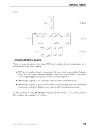
![Heat Transfer
Angular Discretization and Pixelation
Each octant of the angular space 4π at any spatial location is discretized into Nθ × Nφ
solid angles of extent ωi, called control angles. The angles θ and φ are the polar and
azimuthal angles respectively, and are measured with respect to the global Cartesian
system (x, y, z) as shown in Figure 5.3.3. The θ and φ extents of the control angle, ∆θ
and ∆φ, are constant. In two-dimensional calculations, only four octants are solved due to
symmetry, making a total of 4NθNφ directions in all. In three-dimensional calculations,
a total of 8NθNφ directions are solved. In the case of the non-gray model, 4NθNφ or
8NθNφ equations are solved for each band.
θ
φ
z
y
x
s
Figure 5.3.3: Angular Coordinate System
When Cartesian meshes are used, it is possible to align the global angular discretization
with the control volume face, as shown in Figure 5.3.4. For generalized unstructured
meshes, however, control volume faces do not in general align with the global angular
discretization, as shown in Figure 5.3.5, leading to the problem of control angle over-
hang [242].
Essentially, control angles can straddle the control volume faces, so that they are partially
incoming and partially outgoing to the face. Figure 5.3.6 shows a 3D example of a face
with control angle overhang.
The control volume face cuts the sphere representing the angular space at an arbitrary
angle. The line of intersection is a great circle. Control angle overhang may also occur
as a result of reflection and refraction. It is important in these cases to correctly account
for the overhanging fraction. This is done through the use of pixelation [242].
Each overhanging control angle is divided into Nθp ×Nφp pixels, as shown in Figure 5.3.7.
5-26 Release 12.0 c ANSYS, Inc. January 29, 2009](https://image.slidesharecdn.com/flth-130501182911-phpapp02/85/Flth-214-320.jpg)
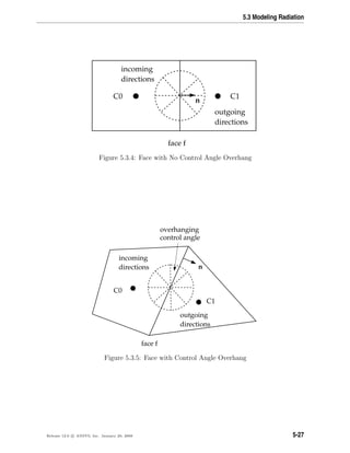
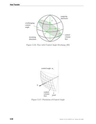
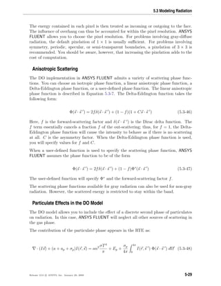
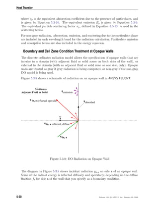
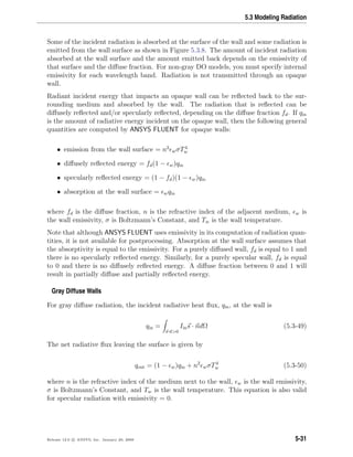
![Heat Transfer
The boundary intensity for all outgoing directions s at the wall is given by
I0 =
qout
π
(5.3-51)
Non-Gray Diffuse Walls
There is a special set of equations that apply uniquely to non-gray diffuse opaque walls.
These equations assume that the absorptivity is equal to the emissivity for the wall
surface. For non-gray diffuse radiation, the incident radiative heat flux qin,λ in the band
∆λ at the wall is
qin,λ = ∆λ
s·n>0
Iin,λs · ndΩ (5.3-52)
The net radiative flux leaving the surface in the band ∆λ is given by
qout,λ = (1 − wλ)qin,λ + wλ[F(0 → nλ2Tw) − F(0 → nλ1Tw)]n2
σT4
w (5.3-53)
where wλ is the wall emissivity in the band. F(n, λ, T) provides the Planck distribution
function. This defines the emittance for each radiation band as a function of the tem-
perature of the source surface. The boundary intensity for all outgoing directions s in
the band ∆λ at the wall is given by
I0λ =
qout,λ
π∆λ
(5.3-54)
Cell Zone and Boundary Condition Treatment at Semi-Transparent Walls
ANSYS FLUENT allows the specification of interior and exterior semi-transparent walls
for the DO model. In the case of interior semi-transparent walls, incident radiation
can pass through the wall and be transmitted to the adjacent medium (and possibly
refracted), it can be reflected back into the surrounding medium, and absorbed through
the wall thickness. Transmission and reflection can be diffuse and/or specular. You
specify the diffuse fraction for all transmitted and reflected radiation; the rest is treated
specularly. For exterior semi-transparent walls, there are two possible sources of radiation
on the boundary wall: an irradiation beam from outside the computational domain and
incident radiation from cells in adjacent fluid or solid zones.
For non-gray radiation, semi-transparent wall boundary conditions are applied on a per-
band basis. The radiant energy within a band is transmitted, reflected, and refracted as
in the gray case; there is no transmission, reflection, or refraction of radiant energy from
one band to another.
5-32 Release 12.0 c ANSYS, Inc. January 29, 2009](https://image.slidesharecdn.com/flth-130501182911-phpapp02/85/Flth-220-320.jpg)
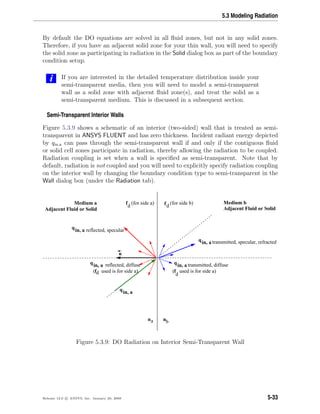
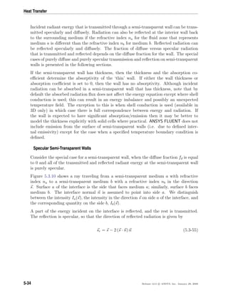
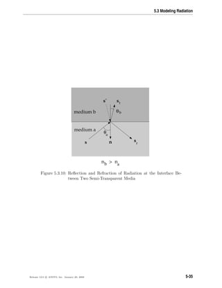
![Heat Transfer
The radiation transmitted from medium a to medium b undergoes refraction. The direc-
tion of the transmitted energy, st, is given by Snell’s law:
sin θb =
na
nb
sin θa (5.3-56)
where θa is the angle of incidence and θb is the angle of transmission, as shown in Fig-
ure 5.3.10. We also define the direction
s = st − 2 (st · n) n (5.3-57)
shown in Figure 5.3.10.
The interface reflectivity on side a [234]
ra(s) =
1
2
na cos θb − nb cos θa
na cos θb + nb cos θa
2
+
1
2
na cos θa − nb cos θb
na cos θa + nb cos θb
2
(5.3-58)
represents the fraction of incident energy transferred from s to sr.
The boundary intensity Iw,a(sr) in the outgoing direction sr on side a of the interface is
determined from the reflected component of the incoming radiation and the transmission
from side b. Thus
Iw,a(sr) = ra(s)Iw,a(s) + τb(s )Iw,b(s ) (5.3-59)
where τb(s ) is the transmissivity of side b in direction s . Similarly, the outgoing intensity
in the direction st on side b of the interface, Iw,b(st), is given by
Iw,b(st) = rb(s )Iw,b(s ) + τa(s)Iw,a(s) (5.3-60)
For the case na < nb, the energy transmitted from medium a to medium b in the incoming
solid angle 2π must be refracted into a cone of apex angle θc (see Figure 5.3.11) where
θc = sin−1 na
nb
(5.3-61)
5-36 Release 12.0 c ANSYS, Inc. January 29, 2009](https://image.slidesharecdn.com/flth-130501182911-phpapp02/85/Flth-224-320.jpg)
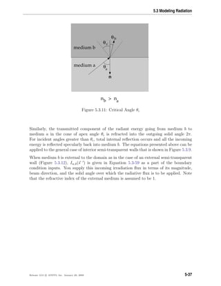
![Heat Transfer
Diffuse Semi-Transparent Walls
Consider the special case for a semi-transparent wall, when the diffuse fraction fd is equal
to 1 and all of the transmitted and reflected radiant energy at the semi-transparent wall
is purely diffuse.
In many engineering problems, the semi-transparent interface may be a diffuse reflector.
For such a case, the interfacial reflectivity r(s) is assumed independent of s, and equal to
the hemispherically averaged value rd. For n = na/nb > 1, rd,a and rd,b are given by [316]
rd,a = 1 −
(1 − rd,b)
n2
(5.3-62)
rd,b =
1
2
+
(3n + 1)(n − 1)
6(n + 1)2
+
n2
(n2
− 1)2
(n2 + 1)3
ln
n − 1
n + 1
−
2n3
(n2
+ 2n − 1)
(n2 + 1)(n4 − 1)
+
8n4
(n4
+ 1)
(n2 + 1)(n4 − 1)2
ln(n) (5.3-63)
The boundary intensity for all outgoing directions on side a of the interface is given by
Iw,a =
rd,aqin,a + τd,bqin,b
π
(5.3-64)
Similarly for side b,
Iw,b =
rd,bqin,b + τd,aqin,a
π
(5.3-65)
where
qin,a = −
4π
Iw,as · ndΩ, s · n < 0 (5.3-66)
qin,b =
4π
Iw,bs · ndΩ, s · n ≥ 0 (5.3-67)
When medium b is external to the domain as in the case of an external semi-transparent
wall (Figure 5.3.12), qin,b is given as a part of the boundary condition inputs. You supply
this incoming irradiation flux in terms of its magnitude, beam direction, and the solid
angle over which the radiative flux is to be applied. Note that the refractive index of the
external medium is assumed to be 1.
5-38 Release 12.0 c ANSYS, Inc. January 29, 2009](https://image.slidesharecdn.com/flth-130501182911-phpapp02/85/Flth-226-320.jpg)
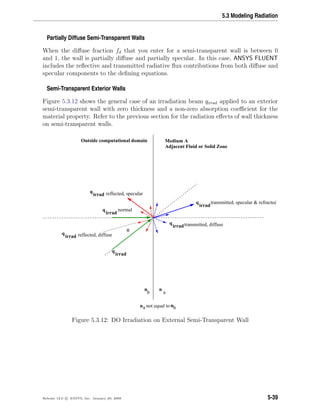
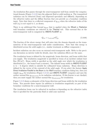
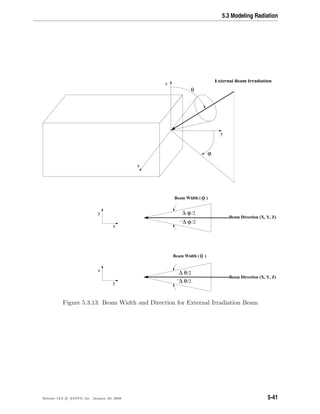
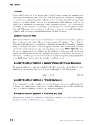
![5.3 Modeling Radiation
5.3.7 Surface-to-Surface (S2S) Radiation Model Theory
The surface-to-surface radiation model can be used to account for the radiation exchange
in an enclosure of gray-diffuse surfaces. The energy exchange between two surfaces de-
pends in part on their size, separation distance, and orientation. These parameters are
accounted for by a geometric function called a “view factor”.
The main assumption of the S2S model is that any absorption, emission, or scattering of
radiation can be ignored; therefore, only “surface-to-surface” radiation need be considered
for analysis.
For information about setting up the model, see Section 13.3.3: Setting Up the S2S Model
in the separate User’s Guide.
Gray-Diffuse Radiation
ANSYS FLUENT’s S2S radiation model assumes the surfaces to be gray and diffuse.
Emissivity and absorptivity of a gray surface are independent of the wavelength. Also,
by Kirchoff’s law [234], the emissivity equals the absorptivity ( = α). For a diffuse
surface, the reflectivity is independent of the outgoing (or incoming) directions.
The gray-diffuse model is what is used in ANSYS FLUENT. Also, as stated earlier, for
applications of interest, the exchange of radiative energy between surfaces is virtually
unaffected by the medium that separates them. Thus, according to the gray-body model,
if a certain amount of radiant energy (E) is incident on a surface, a fraction (ρE) is
reflected, a fraction (αE) is absorbed, and a fraction (τE) is transmitted. Since for most
applications the surfaces in question are opaque to thermal radiation (in the infrared
spectrum), the surfaces can be considered opaque. The transmissivity, therefore, can
be neglected. It follows, from the conservation of energy, that α + ρ = 1, since α =
(emissivity), and ρ = 1 − .
The S2S Model Equations
The energy flux leaving a given surface is composed of directly emitted and reflected
energy. The reflected energy flux is dependent on the incident energy flux from the
surroundings, which then can be expressed in terms of the energy flux leaving all other
surfaces. The energy reflected from surface k is
qout,k = kσT4
k + ρkqin,k (5.3-70)
where qout,k is the energy flux leaving the surface, k is the emissivity, σ is Boltzmann’s
constant, and qin,k is the energy flux incident on the surface from the surroundings.
Release 12.0 c ANSYS, Inc. January 29, 2009 5-43](https://image.slidesharecdn.com/flth-130501182911-phpapp02/85/Flth-231-320.jpg)
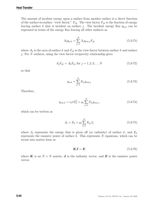
![Heat Transfer
Smoothing
Smoothing can be performed on the view factor matrix to enforce the reciprocity rela-
tionship and conservation.
The reciprocity relationship is represented by
AiFij = AjFji (5.3-79)
where Ai is the area of surface i, Fij is the view factor between surfaces i and j, and Fji
is the view factor between surfaces j and i.
Once the reciprocity relationship has been enforced, a least-squares smoothing method [175]
can be used to ensure that conservation is satisfied, i.e.,
Fij = 1.0 (5.3-80)
5.3.8 Radiation in Combusting Flows
The Weighted-Sum-of-Gray-Gases Model
The weighted-sum-of-gray-gases model (WSGGM) is a reasonable compromise between
the oversimplified gray gas model and a complete model which takes into account partic-
ular absorption bands. The basic assumption of the WSGGM is that the total emissivity
over the distance s can be presented as
=
I
i=0
a ,i(T)(1 − e−κips
) (5.3-81)
where a ,i is the emissivity weighting factor for the ith fictitious gray gas, the bracketed
quantity is the ith fictitious gray gas emissivity, κi is the absorption coefficient of the ith
gray gas, p is the sum of the partial pressures of all absorbing gases, and s is the path
length. For a ,i and κi ANSYS FLUENT uses values obtained from [60] and [326]. These
values depend on gas composition, and a ,i also depend on temperature. When the total
pressure is not equal to 1 atm, scaling rules for κi are used (see Equation 5.3-87).
The absorption coefficient for i = 0 is assigned a value of zero to account for windows in
the spectrum between spectral regions of high absorption ( I
i=1 a ,i < 1) and the weight-
ing factor for i = 0 is evaluated from [326]:
a ,0 = 1 −
I
i=1
a ,i (5.3-82)
5-46 Release 12.0 c ANSYS, Inc. January 29, 2009](https://image.slidesharecdn.com/flth-130501182911-phpapp02/85/Flth-234-320.jpg)
![5.3 Modeling Radiation
The temperature dependence of a ,i can be approximated by any function, but the most
common approximation is
a ,i =
J
j=1
b ,i,jTj−1
(5.3-83)
where b ,i,j are the emissivity gas temperature polynomial coefficients. The coefficients
b ,i,j and κi are estimated by fitting Equation 5.3-81 to the table of total emissivities,
obtained experimentally [60, 70, 326].
The absorptivity α of the radiation from the wall can be approximated in a similar
way [326], but, to simplify the problem, it is assumed that = α [233]. This assumption is
justified unless the medium is optically thin and the wall temperature differs considerably
from the gas temperature.
Since the coefficients b ,i,j and κi are slowly varying functions of ps and T, they can be
assumed constant for a wide range of these parameters. In [326] these constant coefficients
are presented for different relative pressures of the CO2 and H2O vapor, assuming that
the total pressure pT is 1 atm. The values of the coefficients shown in [326] are valid for
0.001 ≤ ps ≤ 10.0 atm-m and 600 ≤ T ≤ 2400 K. For T > 2400 K, coefficient values
suggested by [60] are used. If κips 1 for all i, Equation 5.3-81 simplifies to
=
I
i=0
a ,iκips (5.3-84)
Comparing Equation 5.3-84 with the gray gas model with absorption coefficient a, it can
be seen that the change of the radiation intensity over the distance s in the WSGGM is
exactly the same as in the gray gas model with the absorption coefficient
a =
I
i=0
a ,iκip (5.3-85)
which does not depend on s. In the general case, a is estimated as
a = −
ln(1 − )
s
(5.3-86)
where the emissivity for the WSGGM is computed using Equation 5.3-81. a as defined
by Equation 5.3-86 depends on s, reflecting the non-gray nature of the absorption of
thermal radiation in molecular gases. In ANSYS FLUENT, Equation 5.3-85 is used when
s ≤ 10−4
m and Equation 5.3-86 is used for s > 10−4
m. Note that for s ≈ 10−4
m,
the values of a predicted by Equations 5.3-85 and 5.3-86 are practically identical (since
Equation 5.3-86 reduces to Equation 5.3-85 in the limit of small s).
Release 12.0 c ANSYS, Inc. January 29, 2009 5-47](https://image.slidesharecdn.com/flth-130501182911-phpapp02/85/Flth-235-320.jpg)
![Heat Transfer
ANSYS FLUENT allows you to specify s as the mean beam length or the characteristic
cell size. The model based on the mean beam length is the recommended approach,
especially when you have a nearly homogeneous medium and you are interested in the
radiation exchange between the walls of the enclosure. You can specify the mean beam
length or have ANSYS FLUENT compute it. If you do decide to use the WSGGM based
on the characteristic cell size, note that the predicted values of a will be mesh dependent
(this is a known limitation of the model). See Section 8.8.1: Inputs for a Composition-
Dependent Absorption Coefficient in the separate User’s Guide for details about setting
properties for the WSGGM.
i The WSGGM cannot be used to specify the absorption coefficient in each
band when using the non-gray DO model. If the WSGGM is used with
the non-gray DO model, the absorption coefficient will be the same in all
bands.
When ptot = 1 atm
The WSGGM, as described above, assumes that ptot—the total (static) gas pressure—is
equal to 1 atm. In cases where ptot is not unity (e.g., combustion at high temperatures),
scaling rules suggested in [84] are used to introduce corrections. When ptot < 0.9 atm or
ptot > 1.1 atm, the values for κi in Equations 5.3-81 and 5.3-85 are rescaled:
κi → κipm
tot (5.3-87)
where m is a non-dimensional value obtained from [84], which depends on the partial
pressures and temperature T of the absorbing gases, as well as on ptot.
The Effect of Soot on the Absorption Coefficient
When soot formation is computed, ANSYS FLUENT can include the effect of the soot con-
centration on the radiation absorption coefficient. The generalized soot model estimates
the effect of the soot on radiative heat transfer by determining an effective absorption
coefficient for soot. The absorption coefficient of a mixture of soot and an absorbing
(radiating) gas is then calculated as the sum of the absorption coefficients of pure gas
and pure soot:
as+g = ag + as (5.3-88)
where ag is the absorption coefficient of gas without soot (obtained from the WSGGM)
and
as = b1ρm[1 + bT (T − 2000)] (5.3-89)
5-48 Release 12.0 c ANSYS, Inc. January 29, 2009](https://image.slidesharecdn.com/flth-130501182911-phpapp02/85/Flth-236-320.jpg)
![5.3 Modeling Radiation
with
b1 = 1232.4 m2
/kg and bT ≈ 4.8 × 10⁻⁴
K−1
ρm is the soot density in kg/m3
.
The coefficients b1 and bT were obtained [302] by fitting Equation 5.3-89 to data based
on the Taylor-Foster approximation [348] and data based on the Smith et al. approxima-
tion [326].
See Section 8.8: Radiation Properties and Section 21.3.1: Using the Soot Models in the
separate User’s Guide for information about including the soot-radiation interaction ef-
fects.
The Effect of Particles on the Absorption Coefficient
ANSYS FLUENT can also include the effect of discrete phase particles on the radiation
absorption coefficient, provided that you are using either the P-1 or the DO model. When
the P-1 or DO model is active, radiation absorption by particles can be enabled. The
particle emissivity, reflectivity, and scattering effects are then included in the calculation
of the radiative heat transfer. See Section 23.5: Setting Material Properties for the
Discrete Phase in the separate User’s Guide for more details on the input of radiation
properties for the discrete phase.
5.3.9 Choosing a Radiation Model
For certain problems one radiation model may be more appropriate than the others.
When deciding which radiation model to use, consider the following:
• Optical thickness: The optical thickness aL is a good indicator of which model to
use in your problem. Here, L is an appropriate length scale for your domain. For
flow in a combustor, for example, L is the diameter of the combustion chamber.
If aL 1, your best alternatives are the P-1 and Rosseland models. The P-1
model should typically be used for optical thicknesses > 1. For optical thickness
> 3, the Rosseland model is cheaper and more efficient. For high optical thickness
cases, a second-order discretization scheme for the DO model is recommended. The
DTRM and the DO model work across the full range of optical thicknesses, but are
substantially more expensive to use. Consequently, you should use the “thick-limit”
models, P-1 and Rosseland, if the problem allows it. For optically thin problems
(aL < 1), the DTRM and the DO model, only, are appropriate.
• Scattering and emissivity: The P-1, Rosseland, and DO models account for scat-
tering, while the DTRM neglects it. Since the Rosseland model uses a temperature
slip condition at walls, it is insensitive to wall emissivity.
Release 12.0 c ANSYS, Inc. January 29, 2009 5-49](https://image.slidesharecdn.com/flth-130501182911-phpapp02/85/Flth-237-320.jpg)
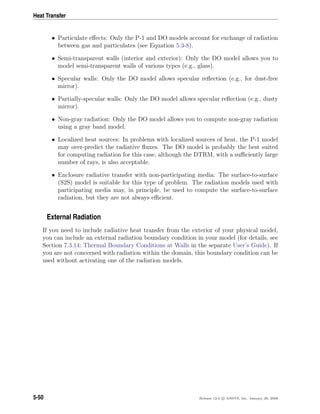
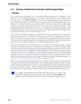
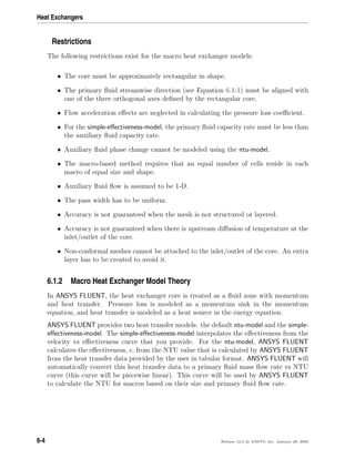
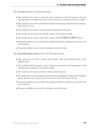
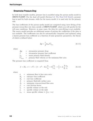
![6.1 The Macro Heat Exchanger Models
Kc and Ke are empirical quantities obtained from experimental data. You will need to
specify these parameters based on graphs that are closest to the heat exchanger config-
uration that you are setting up [160], [158]. These parameters are used to set up large
resistances in the two non-streamwise directions, effectively forcing the primary fluid flow
through the core to be unidirectional.
In Equation 6.1-2, the core friction factor is defined as
fc = aReb
min (6.1-3)
where
a = core friction coefficient
b = core friction exponent
Remin = Reynolds number for velocity at the minimum flow area
a and b are empirical quantities obtained from experimental data. You will need to
specify the core friction coefficient and exponent based on graphs that are closest to the
heat exchanger models that you set up [160], [158].
The Reynolds number in Equation 6.1-3 is defined as
Remin =
ρmUAmin
Dh
µm
(6.1-4)
where
ρm = mean primary fluid density
µm = mean primary fluid viscosity
Dh = hydraulic diameter
UAmin
= primary fluid velocity at the minimum flow area
For a heat exchanger core, the hydraulic diameter can be defined as
Dh = 4L
Ac
A
(6.1-5)
where L is the flow length of the heat exchanger. If the tubes are normal to the primary
fluid flow, then L is the length in the primary fluid flow direction. Note that UAmin
can
be calculated from
UAmin
=
U
σ
(6.1-6)
where U is the primary fluid velocity and σ is the minimum flow to face area ratio.
Release 12.0 c ANSYS, Inc. January 29, 2009 6-7](https://image.slidesharecdn.com/flth-130501182911-phpapp02/85/Flth-245-320.jpg)
![Heat Exchangers
Heat Transfer Effectiveness
For the simple-effectiveness-model, the heat-exchanger effectiveness, , is defined as the
ratio of actual rate of heat transfer from the hot to cold fluid to the maximum possible
rate of heat transfer. The maximum possible heat transfer is given by
qmax = Cmin(Tin,hot − Tin,cold) (6.1-7)
where Tin,hot and Tin,cold are the inlet temperatures of the hot and cold fluids and
Cmin = min[( ˙mcp)hot, ( ˙mcp)cold] (6.1-8)
Thus, the actual rate of heat transfer, q, is defined as
q = Cmin(Tin,hot − Tin,cold) (6.1-9)
The value of depends on the heat exchanger geometry and flow pattern (parallel flow,
counter flow, cross flow, etc.). Even though the effectiveness of the primary fluid is
computed using uniform conditions on the entire heat exchanger core, it is being applied
to a small portion of the core represented by a computational cell. This can make it less
accurate for some heat exchanger cores, where there is a strong variation in the primary
flow. For a core with a strong primary flow variation, the NTU model must be used.
For the ntu-model, given the heat exchanger performance data (total heat rejection versus
primary flow rate) based on uniform test conditions, ANSYS FLUENT calculates the
effectiveness of the entire heat exchanger from the ratio of heat capacity and the number
of transfer units using the relation
= 1 − exp −
1
Cr
N0.22
tu (1 − e−CrN0.78
tu ) (6.1-10)
where Cr is the ratio of Cmin to Cmax.
The heat exchanger performance data should be specified for a number of auxiliary flow
rates so that ANSYS FLUENT can compute the number of transfer units versus the
primary fluid flow rate for a number of auxiliary fluid flow rates. This NTU, which is
based on the full heat exchanger and uniform conditions, is scaled for each macro using
the ratio of their volumes and minimum heat capacities.
For each macro, the primary fluid inlet temperature is calculated using the mass average
of the incoming primary fluid temperatures at the boundaries. This automatically takes
into account any reverse flow of the primary fluid at the boundaries.
6-8 Release 12.0 c ANSYS, Inc. January 29, 2009](https://image.slidesharecdn.com/flth-130501182911-phpapp02/85/Flth-246-320.jpg)
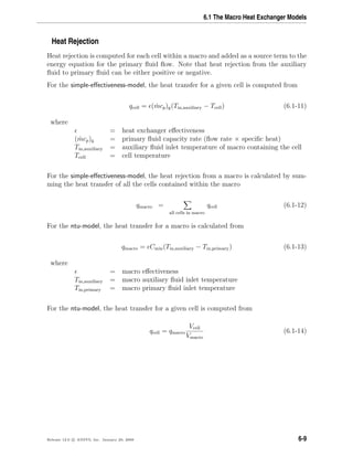
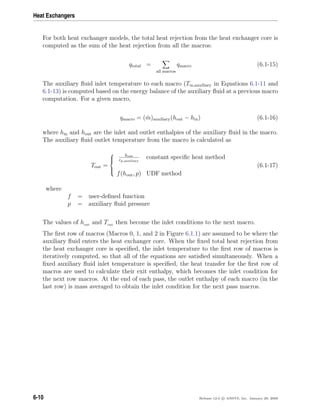
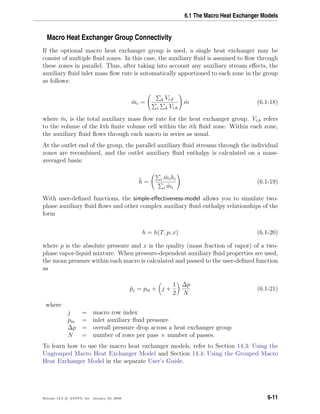
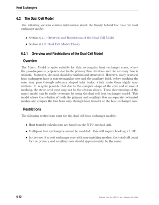
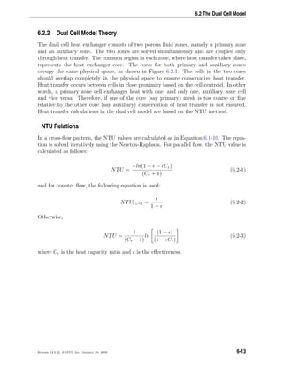
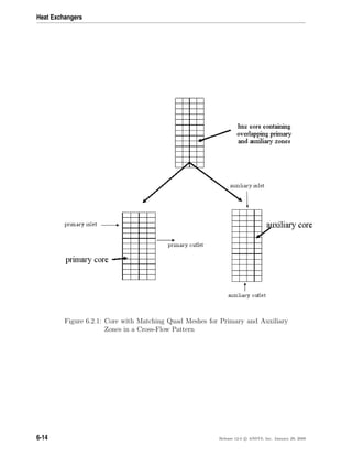
![6.2 The Dual Cell Model
Heat Rejection
Heat rejection is computed for each cell in the two cores (primary and auxiliary) and
added as a source term to the energy equation for the respective flows. This is illustrated
in Figure 6.2.2 and the following equations:
Figure 6.2.2: Core with Primary and Auxiliary Zones with Possible Overlap
of Cells
˙mscaled,A = ρcell,AVcell,AAinlet,A (6.2-4)
˙mscaled,P = ρcell,P Vcell,P Ainlet,P (6.2-5)
Cmin,scaled = min[(Cp,cell ˙mscale)|P , (Cp,cell ˙mscale)|A] (6.2-6)
Release 12.0 c ANSYS, Inc. January 29, 2009 6-15](https://image.slidesharecdn.com/flth-130501182911-phpapp02/85/Flth-253-320.jpg)
![Heat Exchangers
NTUscaled = [NTUfull( ˙mscaled,P , ˙mscaled,A)]bilinearinterpolation (6.2-7)
(UA)scaled = NTUscaled Cmin,scaled (6.2-8)
dq = qcell =
(UA)scaled(Tcell,A − Tcell,P )
V olumecell
(6.2-9)
where Tcell,A = auxiliary cell temperature
Tcell,P = primary cell temperature
U = overall heat transfer coefficient
A = total heat transfer area
Cmin,scaled = scaled minimum heat capacity rate
You can supply the NTU values, or it can be calculated using the supplied raw data and
the effectiveness-NTU relation that you specify.
To learn how to use the dual cell heat exchanges model, refer to Section 14.5: Using the
Dual Cell Heat Exchanger Model in the separate User’s Guide.
6-16 Release 12.0 c ANSYS, Inc. January 29, 2009](https://image.slidesharecdn.com/flth-130501182911-phpapp02/85/Flth-254-320.jpg)
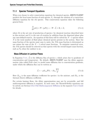
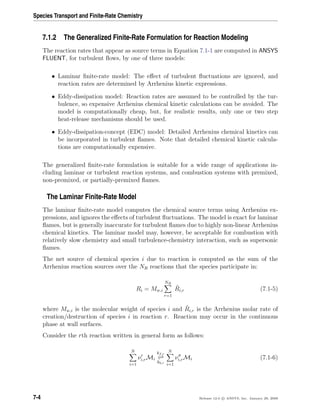

(7.1-7)
where
Cj,r = molar concentration of species j in reaction r (kgmol/m3
)
ηj,r = rate exponent for reactant species j in reaction r
ηj,r = rate exponent for product species j in reaction r
For a reversible reaction, the molar rate of creation/destruction of species i in reaction r
is given by
ˆRi,r = Γ νi,r − νi,r
kf,r
N
j=1
[Cj,r]ηj,r
− kb,r
N
j=1
[Cj,r]νj,r
(7.1-8)
Note that the rate exponent for the reverse reaction part in Equation 7.1-8 is always the
product species stoichiometric coefficient (νj,r).
For information about inputting the stoichiometric coefficients and rate exponents for
both global forward (non-reversible) reactions and elementary (reversible) reactions, see
Section 15.1.3: Inputs for Reaction Definition in the separate User’s Guide.
Γ represents the net effect of third bodies on the reaction rate. This term is given by
Γ =
N
j
γj,rCj (7.1-9)
Release 12.0 c ANSYS, Inc. January 29, 2009 7-5](https://image.slidesharecdn.com/flth-130501182911-phpapp02/85/Flth-259-320.jpg)
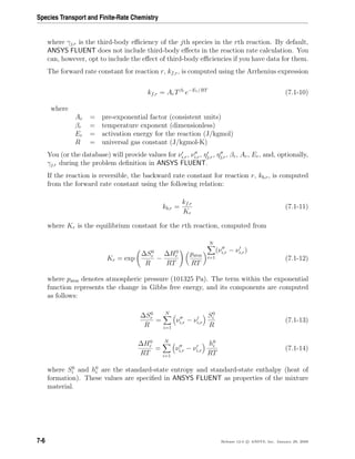
![7.1 Volumetric Reactions
Pressure-Dependent Reactions
ANSYS FLUENT can use one of three methods to represent the rate expression in pressure-
dependent (or pressure fall-off) reactions. A “fall-off” reaction is one in which the tem-
perature and pressure are such that the reaction occurs between Arrhenius high-pressure
and low-pressure limits, and thus is no longer solely dependent on temperature.
There are three methods of representing the rate expressions in this fall-off region. The
simplest one is the Lindemann [198] form. There are also two other related methods, the
Troe method [111] and the SRI method [339], that provide a more accurate description
of the fall-off region.
Arrhenius rate parameters are required for both the high- and low-pressure limits. The
rate coefficients for these two limits are then blended to produce a smooth pressure-
dependent rate expression. In Arrhenius form, the parameters for the high-pressure limit
(k) and the low-pressure limit (klow) are as follows:
k = ATβ
e−E/RT
(7.1-15)
klow = AlowTβlow
e−Elow/RT
(7.1-16)
The net rate constant at any pressure is then taken to be
knet = k
pr
1 + pr
F (7.1-17)
where pr is defined as
pr =
klow[M]
k
(7.1-18)
and [M] is the concentration of the bath gas, which can include third-body efficiencies.
If the function F in Equation 7.1-17 is unity, then this is the Lindemann form. ANSYS
FLUENT provides two other forms to describe F, namely the Troe method and the SRI
method.
In the Troe method, F is given by
log F =
1 +
log pr + c
n − d(log pr + c)
2
−1
log Fcent (7.1-19)
Release 12.0 c ANSYS, Inc. January 29, 2009 7-7](https://image.slidesharecdn.com/flth-130501182911-phpapp02/85/Flth-261-320.jpg)
![Species Transport and Finite-Rate Chemistry
where
c = −0.4 − 0.67 log Fcent (7.1-20)
n = 0.75 − 1.27 log Fcent (7.1-21)
d = 0.14 (7.1-22)
and
Fcent = (1 − α)e−T/T1
+ αe−T/T2
+ e−T3/T
(7.1-23)
The parameters α, T3, T2, and T1 are specified as inputs.
In the SRI method, the blending function F is approximated as
F = d a exp
−b
T
+ exp
−T
c
X
Te
(7.1-24)
where
X =
1
1 + log2
pr
(7.1-25)
In addition to the three Arrhenius parameters for the low-pressure limit (klow) expression,
you must also supply the parameters a, b, c, d, and e in the F expression.
i Chemical kinetic mechanisms usually contain a wide range of time scales
and form a set of highly non-linear, stiff coupled equations. For solution
procedure guidelines, see Section 15.1.7: Solution Procedures for Chemical
Mixing and Finite-Rate Chemistry in the separate User’s Guide. Also,
if you have a chemical mechanism in CHEMKIN [161] format, you can
import this mechanism into ANSYS FLUENT (see Section 15.1.9: Importing
a Volumetric Kinetic Mechanism in CHEMKIN Format in the separate
User’s Guide).
The Eddy-Dissipation Model
Most fuels are fast burning, and the overall rate of reaction is controlled by turbulent
mixing. In non-premixed flames, turbulence slowly convects/mixes fuel and oxidizer into
the reaction zones where they burn quickly. In premixed flames, the turbulence slowly
convects/mixes cold reactants and hot products into the reaction zones, where reaction
7-8 Release 12.0 c ANSYS, Inc. January 29, 2009](https://image.slidesharecdn.com/flth-130501182911-phpapp02/85/Flth-262-320.jpg)
![7.1 Volumetric Reactions
occurs rapidly. In such cases, the combustion is said to be mixing-limited, and the
complex, and often unknown, chemical kinetic rates can be safely neglected.
ANSYS FLUENT provides a turbulence-chemistry interaction model, based on the work
of Magnussen and Hjertager [216], called the eddy-dissipation model. The net rate of
production of species i due to reaction r, Ri,r, is given by the smaller (i.e., limiting value)
of the two expressions below:
Ri,r = νi,rMw,iAρ
k
min
R
YR
νR,rMw,R
(7.1-26)
Ri,r = νi,rMw,iABρ
k
P YP
N
j νj,rMw,j
(7.1-27)
where YP is the mass fraction of any product species, P
YR is the mass fraction of a particular reactant, R
A is an empirical constant equal to 4.0
B is an empirical constant equal to 0.5
In Equations 7.1-26 and 7.1-27, the chemical reaction rate is governed by the large-eddy
mixing time scale, k/ , as in the eddy-breakup model of Spalding [333]. Combustion
proceeds whenever turbulence is present (k/ > 0), and an ignition source is not re-
quired to initiate combustion. This is usually acceptable for non-premixed flames, but
in premixed flames, the reactants will burn as soon as they enter the computational
domain, upstream of the flame stabilizer. To remedy this, ANSYS FLUENT provides
the finite-rate/eddy-dissipation model, where both the Arrhenius (Equation 7.1-8), and
eddy-dissipation (Equations 7.1-26 and 7.1-27) reaction rates are calculated. The net
reaction rate is taken as the minimum of these two rates. In practice, the Arrhenius rate
acts as a kinetic “switch”, preventing reaction before the flame holder. Once the flame
is ignited, the eddy-dissipation rate is generally smaller than the Arrhenius rate, and
reactions are mixing-limited.
i Although ANSYS FLUENT allows multi-step reaction mechanisms (number
of reactions > 2) with the eddy-dissipation and finite-rate/eddy-dissipation
models, these will likely produce incorrect solutions. The reason is that
multi-step chemical mechanisms are based on Arrhenius rates, which dif-
fer for each reaction. In the eddy-dissipation model, every reaction has
the same, turbulent rate, and therefore the model should be used only
for one-step (reactant → product), or two-step (reactant → intermedi-
ate, intermediate → product) global reactions. The model cannot predict
kinetically controlled species such as radicals. To incorporate multi-step
chemical kinetic mechanisms in turbulent flows, use the EDC model (de-
scribed below).
Release 12.0 c ANSYS, Inc. January 29, 2009 7-9](https://image.slidesharecdn.com/flth-130501182911-phpapp02/85/Flth-263-320.jpg)
![Species Transport and Finite-Rate Chemistry
i The eddy-dissipation model requires products to initiate reaction (see
Equation 7.1-27). When you initialize the solution for steady flows, ANSYS
FLUENT sets all species mass fractions to a maximum of the user speci-
fied initial value and 0.01. This is usually sufficient to start the reaction.
However, if you converge a mixing solution first, where all product mass
fractions are zero, you may then have to patch products into the reac-
tion zone to ignite the flame. For details, see Section 15.1.7: Ignition in
Combustion Simulations in the separate User’s Guide.
The Eddy-Dissipation Model for LES
When the LES turbulence model is used, the turbulent mixing rate, /k in Equa-
tions 7.1-26 and 7.1-27, is replaced by the subgrid-scale mixing rate. This is calculated
as
τ−1
sgs = 2SijSij (7.1-28)
where
τ−1
sgs = subgrid-scale mixing rate (s−1
)
Sij = 1
2
∂ui
∂xj
+ ∂uj
∂xi
= strain rate tensor (s−1
)
The Eddy-Dissipation-Concept (EDC) Model
The eddy-dissipation-concept (EDC) model is an extension of the eddy-dissipation model
to include detailed chemical mechanisms in turbulent flows [215]. It assumes that reaction
occurs in small turbulent structures, called the fine scales. The length fraction of the fine
scales is modeled as [115]
ξ∗
= Cξ
ν
k2
1/4
(7.1-29)
where ∗
denotes fine-scale quantities and
Cξ = volume fraction constant = 2.1377
ν = kinematic viscosity
The volume fraction of the fine scales is calculated as ξ∗3
. Species are assumed to react
in the fine structures over a time scale
τ∗
= Cτ
ν 1/2
(7.1-30)
where Cτ is a time scale constant equal to 0.4082.
7-10 Release 12.0 c ANSYS, Inc. January 29, 2009](https://image.slidesharecdn.com/flth-130501182911-phpapp02/85/Flth-264-320.jpg)
![7.2 Wall Surface Reactions and Chemical Vapor Deposition
In ANSYS FLUENT, combustion at the fine scales is assumed to occur as a constant
pressure reactor, with initial conditions taken as the current species and temperature in
the cell. Reactions proceed over the time scale τ∗
, governed by the Arrhenius rates of
Equation 7.1-8, and are integrated numerically using the ISAT algorithm [277]. ISAT
can accelerate the chemistry calculations by two to three orders of magnitude, offering
substantial reductions in run-times. Details about the ISAT algorithm may be found
in Sections 11.3.3 and 11.3.4. ISAT is very powerful, but requires some care. See Sec-
tion 19.6.2: Using ISAT Efficiently in the separate User’s Guide for details on using ISAT
efficiently.
The source term in the conservation equation for the mean species i, Equation 7.1-1, is
modeled as
Ri =
ρ(ξ∗
)2
τ∗[1 − (ξ∗)3
]
(Y ∗
i − Yi) (7.1-31)
where Y ∗
i is the fine-scale species mass fraction after reacting over the time τ∗
.
The EDC model can incorporate detailed chemical mechanisms into turbulent reacting
flows. However, typical mechanisms are invariably stiff and their numerical integration
is computationally costly. Hence, the model should be used only when the assumption
of fast chemistry is invalid, such as modeling the slow CO burnout in rapidly quenched
flames, or the NO conversion in selective non-catalytic reduction (SNCR).
For guidelines on obtaining a solution using the EDC model, see Section 15.1.7: Solution
of Stiff Laminar Chemistry Systems in the separate User’s Guide.
7.2 Wall Surface Reactions and Chemical Vapor Deposition
For gas-phase reactions, the reaction rate is defined on a volumetric basis and the rate
of creation and destruction of chemical species becomes a source term in the species
conservation equations. For surface reactions, the rate of adsorption and desorption is
governed by both chemical kinetics and diffusion to and from the surface. Wall surface
reactions thus create sources and sinks of chemical species in the gas phase, as well as on
the reacting surface.
Theoretical information about wall surface reactions and chemical vapor deposition is
presented in this section. Information can be found in the following sections:
• Section 7.2.1: Surface Coverage Reaction Rate Modification
• Section 7.2.2: Reaction-Diffusion Balance for Surface Chemistry
• Section 7.2.3: Slip Boundary Formulation for Low-Pressure Gas Systems
Release 12.0 c ANSYS, Inc. January 29, 2009 7-11](https://image.slidesharecdn.com/flth-130501182911-phpapp02/85/Flth-265-320.jpg)
![Species Transport and Finite-Rate Chemistry
For more information about using wall surface reactions and chemical vapor deposition,
see Section 15.2: Wall Surface Reactions and Chemical Vapor Deposition in the separate
User’s Guide.
Consider the rth wall surface reaction written in general form as follows:
Ng
i=1
gi,rGi +
Nb
i=1
bi,rBi +
Ns
i=1
si,rSi
Kr
Ng
i=1
gi,rGi +
Nb
i=1
bi,rBi +
Ns
i=1
si,rSi (7.2-1)
where Gi, Bi, and Si represent the gas phase species, the bulk (or solid) species, and the
surface-adsorbed (or site) species, respectively. Ng, Nb, and Ns are the total numbers of
these species. gi,r, bi,r, and si,r are the stoichiometric coefficients for each reactant species
i, and gi,r, bi,r, and si,r are the stoichiometric coefficients for each product species i. Kr
is the overall forward reaction rate constant. Note that ANSYS FLUENT cannot model
reversible surface reactions.
The summations in Equation 7.2-1 are for all chemical species in the system, but only
species involved as reactants or products will have non-zero stoichiometric coefficients.
Hence, species that are not involved will drop out of the equation.
The rate of the rth reaction is
Rr = kf,r
Ng
i=1
[Ci]
ηi,g,r
wall
Ns
j=1
[Sj]
ηj,s,r
wall
(7.2-2)
where [ ]wall represents molar concentrations of surface-adsorbed species on the wall. ηi,g,r
is the rate exponent for the ith
gaseous species as reactant in the reaction and ηj,s,r is the
rate exponent for the jth
site species as reactant in the reaction. It is assumed that the
reaction rate does not depend on concentrations of the bulk (solid) species. From this,
the net molar rate of production or consumption of each species i is given by
ˆRi,gas =
Nrxn
r=1
(gi,r − gi,r)Rr i = 1, 2, 3, . . . , Ng (7.2-3)
ˆRi,bulk =
Nrxn
r=1
(bi,r − bi,r)Rr i = 1, 2, 3, . . . , Nb (7.2-4)
ˆRi,site =
Nrxn
r=1
(si,r − si,r)Rr i = 1, 2, 3, . . . , Ns (7.2-5)
The forward rate constant for reaction r (kf,r) is computed using the Arrhenius expres-
sion,
7-12 Release 12.0 c ANSYS, Inc. January 29, 2009](https://image.slidesharecdn.com/flth-130501182911-phpapp02/85/Flth-266-320.jpg)
![7.2 Wall Surface Reactions and Chemical Vapor Deposition
kf,r = ArTβr
e−Er/RT
(7.2-6)
where Ar = pre-exponential factor (consistent units)
βr = temperature exponent (dimensionless)
Er = activation energy for the reaction (J/kgmol)
R = universal gas constant (J/kgmol-K)
You (or the database) will provide values for gi,r, gi,r, bi,r, bi,r, si,r, si,r, βr, Ar, and Er.
To include the mass transfer effects and model heat release, refer to Section 15.2.3: Includ-
ing Mass Transfer To Surfaces in Continuity, Section 15.2.4: Wall Surface Mass Transfer
Effects in the Energy Equation, and Section 15.2.5: Modeling the Heat Release Due to
Wall Surface Reactions in the separate User’s Guide
7.2.1 Surface Coverage Reaction Rate Modification
ANSYS FLUENT has the option to modify the surface reaction rate as a function of
species site coverages. In such cases, the forward rate constant for the rth reaction is
evaluated as,
kf,r = ArTβr
e−Er/RT
ksite
10Zkηk,r
(Zk
µk,r
) e− k,rZk/RT
(7.2-7)
In Equation 7.2-7, the three surface coverage rate modification parameters for specie k in
reaction r are ηk,r, µk,r and k,r. These parameters default to zero for reaction species that
are not surface rate modifying. The surface (coverage) site fraction, Zk is the fraction of
surface sites covered by specie k, and is defined as,
Zk = [Sk]/ρsite (7.2-8)
where [Sk] is the surface site concentration and ρsite is the surface site density (see Equa-
tion 7.2-13).
Release 12.0 c ANSYS, Inc. January 29, 2009 7-13](https://image.slidesharecdn.com/flth-130501182911-phpapp02/85/Flth-267-320.jpg)
![Species Transport and Finite-Rate Chemistry
7.2.2 Reaction-Diffusion Balance for Surface Chemistry
Reactions at surfaces change gas-phase, surface-adsorbed (site) and bulk (solid) species.
On reacting surfaces, the mass flux of each gas specie due to diffusion and convection
to/from the surface is balanced with its rate of consumption/production on the surface,
ρwallDi
∂Yi,wall
∂n
− ˙mdepYi,wall = Mw,i
ˆRi,gas i = 1, 2, 3, . . . , Ng (7.2-9)
∂ [Si]wall
∂t
= ˆRi,site i = 1, 2, 3, . . . , Ns (7.2-10)
The wall mass fraction Yi,wall is related to concentration by
[Gi]wall =
ρwallYi,wall
Mw,i
(7.2-11)
˙mdep is the net rate of mass deposition or etching as a result of surface reaction; i.e.,
˙mdep =
Nb
i=1
Mw,i
ˆRi,bulk (7.2-12)
[Si]wall is the site species concentration at the wall, and is defined as
[Si]wall = ρsiteZi (7.2-13)
where ρsite is the site density and Zi is the site coverage of species i.
Equations 7.2-9 and 7.2-10 are solved for the dependent variables Yi,wall and Zi using a
point-by-point coupled Newton solver. The effective gas-phase reaction source terms are
then available for solution of the gas-phase species transport Equation 7.1-1.
7-14 Release 12.0 c ANSYS, Inc. January 29, 2009](https://image.slidesharecdn.com/flth-130501182911-phpapp02/85/Flth-268-320.jpg)
![7.2 Wall Surface Reactions and Chemical Vapor Deposition
7.2.3 Slip Boundary Formulation for Low-Pressure Gas Systems
Most semiconductor fabrication devices operate far below atmospheric pressure, typically
only a few millitorrs. At such low pressures, the fluid flow is in the slip regime and the
normally used no-slip boundary conditions for velocity and temperature are no longer
valid.
The Knudsen number, denoted Kn, and defined as the ratio of mean free path to a
characteristic length scale of the system, is used to quantify continuum flow regimes.
Since the mean free path increases as the pressure is lowered, the high end of Kn values
represents free molecular flow and the low end the continuum regime. The range in
between these two extremes is called the slip regime (0.01 < Kn < 0.1) [28] In the slip
regime, the gas-phase velocity at a solid surface differs from the velocity at which the
wall moves, and the gas temperature at the surface differs from the wall temperature.
Maxwell’s models are adopted for these physical phenomena in ANSYS FLUENT for their
simplicity and effectiveness.
• velocity slip
Uw − Ug =
2 − αv
αv
Kn
∂U
∂n
≈
2 − αv
αv
λ
δ
(Ug − Uc) (7.2-14)
Vg ≡ (V · n)g = Vw (7.2-15)
Here, U and V represents the velocity component that is parallel and normal to
the wall, respectively. The subscripts g, w and c indicate gas, wall and cell-center
velocities. δ is the distance from cell center to the wall. αv is the momentum
accommodation coefficient of the gas mixture and its value is calculated as mass-
fraction weighted average of each gas species in the system.
αv =
Ng
i=1
Yiαi (7.2-16)
The mean free path, λ, is computed as follows:
λ =
kBT
√
2πσ2p
(7.2-17)
σ =
Ng
i=1
Yiσi (7.2-18)
σi is the Lennard-Jones characteristic length of species i. kB is the Boltzmann
constant, 1.38066 × 10⁻²³
J/K.
Release 12.0 c ANSYS, Inc. January 29, 2009 7-15](https://image.slidesharecdn.com/flth-130501182911-phpapp02/85/Flth-269-320.jpg)
![Species Transport and Finite-Rate Chemistry
Equations 7.2-14 and 7.2-15 indicate that while the gas velocity component normal
to the wall is the same as the wall normal velocity, the tangential components slip.
The values lie somewhere between the cell-center and the wall values. These two
equations can be combined to give a generalized formulation:
Vg =
Vw + k
δ
[(Vw · n)n + Vc − (Vc · n)n]
1 + k
δ
(7.2-19)
where
k ≡ λ
2 − αv
αv
(7.2-20)
• temperature jump
Tw − Tg = 2
2 − αT
αT
Kn
∂T
∂n
≈ 2
2 − αT
αT
λ
δ
(Tg − Tc) (7.2-21)
or equivalently
Tg =
Tw + βTc
1 + β
(7.2-22)
where
β =
2(2 − αT )
αT δ
(7.2-23)
αT is the thermal accommodation coefficient of the gas mixture and is calculated
as αT = YiαT,i.
i The low-pressure slip boundary formulation is available only with the
pressure-based solver.
7-16 Release 12.0 c ANSYS, Inc. January 29, 2009](https://image.slidesharecdn.com/flth-130501182911-phpapp02/85/Flth-270-320.jpg)
![7.3 Particle Surface Reactions
7.3 Particle Surface Reactions
As described in Section 15.4.5: The Multiple Surface Reactions Model, it is possible to
define multiple particle surface reactions to model the surface combustion of a combust-
ing discrete-phase particle. This section provides theoretical background about particle
surface reactions. Information can be found in the following sections:
• Section 7.3.1: General Description
• Section 7.3.2: ANSYS FLUENT Model Formulation
• Section 7.3.3: Extension for Stoichiometries with Multiple Gas Phase Reactants
• Section 7.3.4: Solid-Solid Reactions
• Section 7.3.5: Solid Decomposition Reactions
• Section 7.3.6: Solid Deposition Reactions
• Section 7.3.7: Gaseous Solid Catalyzed Reactions on the Particle Surface
For more information about using particle surface reactions, see Section 15.3: Particle
Surface Reactions in the separate User’s Guide.
7.3.1 General Description
The relationships for calculating char particle burning rates are presented and discussed
in detail by Smith [324]. The particle reaction rate, R (kg/m2
-s), can be expressed as
R = D0(Cg − Cs) = Rc(Cs)N
(7.3-1)
where
D0 = bulk diffusion coefficient (m/s)
Cg = mean reacting gas species concentration in the bulk (kg/m3
)
Cs = mean reacting gas species concentration at the particle surface (kg/m3
)
Rc = chemical reaction rate coefficient (units vary)
N = apparent reaction order (dimensionless)
In Equation 7.3-1, the concentration at the particle surface, Cs, is not known, so it should
be eliminated, and the expression is recast as follows:
R = Rc Cg −
R
D0
N
(7.3-2)
Release 12.0 c ANSYS, Inc. January 29, 2009 7-17](https://image.slidesharecdn.com/flth-130501182911-phpapp02/85/Flth-271-320.jpg)
![7.3 Particle Surface Reactions
Rj,r = Rkin,r pn −
Rj,r
D0,r
N
(7.3-5)
where
Rj,r = rate of particle surface species depletion (kg/s)
Ap = particle surface area (m2
)
Yj = mass fraction of surface species j in the particle
ηr = effectiveness factor (dimensionless)
Rj,r = rate of particle surface species reaction per unit area (kg/m2
-s)
pn = bulk partial pressure of the gas phase species (Pa)
D0,r = diffusion rate coefficient for reaction r
Rkin,r = kinetic rate of reaction r (units vary)
Nr = apparent order of reaction r
The effectiveness factor, ηr, is related to the surface area, and can be used in each reaction
in the case of multiple reactions. D0,r is given by
D0,r = C1,r
[(Tp + T∞)/2]0.75
dp
(7.3-6)
The kinetic rate of reaction r is defined as
Rkin,r = ArTp
βr
e−(Er/RTp)
(7.3-7)
The rate of the particle surface species depletion for reaction order Nr = 1 is given by
Rj,r = ApηrYjpn
Rkin,rD0,r
D0,r + Rkin,r
(7.3-8)
For reaction order Nr = 0,
Rj,r = ApηrYjRkin,r (7.3-9)
Release 12.0 c ANSYS, Inc. January 29, 2009 7-19](https://image.slidesharecdn.com/flth-130501182911-phpapp02/85/Flth-273-320.jpg)
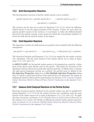

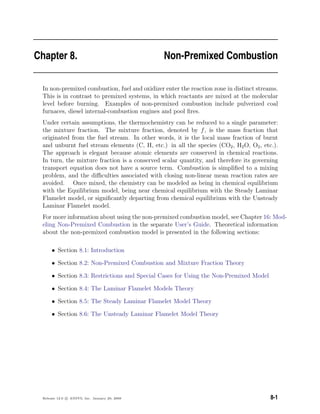
![Non-Premixed Combustion
8.1 Introduction
Non-premixed modeling involves the solution of transport equations for one or two con-
served scalars (the mixture fractions). Equations for individual species are not solved.
Instead, species concentrations are derived from the predicted mixture fraction fields. The
thermochemistry calculations are preprocessed and then tabulated for look-up in ANSYS
FLUENT. Interaction of turbulence and chemistry is accounted for with an assumed-shape
Probability Density Function (PDF).
8.2 Non-Premixed Combustion and Mixture Fraction Theory
Information about non-premixed combustion and mixture fraction theory are presented
in the following sections:
• Section 8.2.1: Mixture Fraction Theory
• Section 8.2.2: Modeling of Turbulence-Chemistry Interaction
• Section 8.2.3: Non-Adiabatic Extensions of the Non-Premixed Model
• Section 8.2.4: Chemistry Tabulation
8.2.1 Mixture Fraction Theory
Definition of the Mixture Fraction
The basis of the non-premixed modeling approach is that under a certain set of simplifying
assumptions, the instantaneous thermochemical state of the fluid is related to a conserved
scalar quantity known as the mixture fraction, f. The mixture fraction can be written
in terms of the atomic mass fraction as [319]
f =
Zi − Zi,ox
Zi,fuel − Zi,ox
(8.2-1)
where Zi is the elemental mass fraction for element, i. The subscript ox denotes the value
at the oxidizer stream inlet and the subscript fuel denotes the value at the fuel stream
inlet. If the diffusion coefficients for all species are equal, then Equation 8.2-1 is identical
for all elements, and the mixture fraction definition is unique. The mixture fraction is
thus the elemental mass fraction that originated from the fuel stream.
8-2 Release 12.0 c ANSYS, Inc. January 29, 2009](https://image.slidesharecdn.com/flth-130501182911-phpapp02/85/Flth-278-320.jpg)
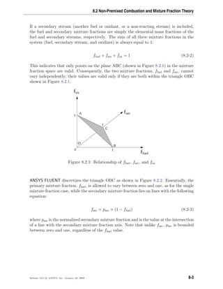
![8.2 Non-Premixed Combustion and Mixture Fraction Theory
An important characteristic of the normalized secondary mixture fraction, psec, is its
assumed statistical independence from the fuel mixture fraction, ffuel. Note that unlike
fsec, psec is not a conserved scalar. This normalized mixture fraction definition, psec,
is used everywhere in ANSYS FLUENT when prompted for Secondary Mixture Fraction
except when defining the rich limit for a secondary fuel stream, which is defined in terms
of fsec.
Transport Equations for the Mixture Fraction
Under the assumption of equal diffusivities, the species equations can be reduced to a
single equation for the mixture fraction, f. The reaction source terms in the species
equations cancel (since elements are conserved in chemical reactions), and thus f is a
conserved quantity. While the assumption of equal diffusivities is problematic for laminar
flows, it is generally acceptable for turbulent flows where turbulent convection overwhelms
molecular diffusion. The Favre mean (density-averaged) mixture fraction equation is
∂
∂t
(ρf) + · (ρvf) = ·
µt
σt
f + Sm + Suser (8.2-4)
The source term Sm is due solely to transfer of mass into the gas phase from liquid fuel
droplets or reacting particles (e.g., coal). Suser is any user-defined source term.
In addition to solving for the Favre mean mixture fraction, ANSYS FLUENT solves a
conservation equation for the mixture fraction variance, f 2 [152]:
∂
∂t
ρf 2 + · ρvf 2 = ·
µt
σt
f 2 + Cgµt f
2
− Cdρ
k
f 2 + Suser (8.2-5)
where f = f − f. The default values for the constants σt, Cg, and Cd are 0.85, 2.86, and
2.0, respectively, and Suser is any user-defined source term.
The mixture fraction variance is used in the closure model describing turbulence-chemistry
interactions (see Section 8.2.2: Modeling of Turbulence-Chemistry Interaction).
For a two-mixture-fraction problem, ffuel and f 2
fuel are obtained from Equations 8.2-4 and
8.2-5 by substituting ffuel for f and f 2
fuel for f 2. fsec is obtained from Equation 8.2-4 by
substituting fsec for f. psec is then calculated using Equation 8.2-3, and p 2
sec is obtained
by solving Equation 8.2-5 with psec substituted for f. To a first-order approximation, the
variances in psec and fsec are relatively insensitive to ffuel, and therefore the equation for
p 2
sec is essentially the same as f 2
sec.
i The equation for p 2
sec instead of f 2
sec is valid when the mass flow rate of
the secondary stream is relatively small compared with the total mass flow
rate.
Release 12.0 c ANSYS, Inc. January 29, 2009 8-5](https://image.slidesharecdn.com/flth-130501182911-phpapp02/85/Flth-281-320.jpg)
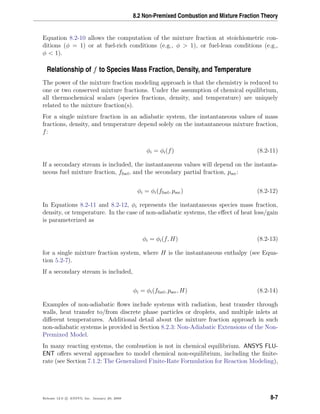
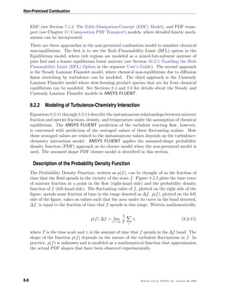
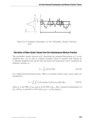
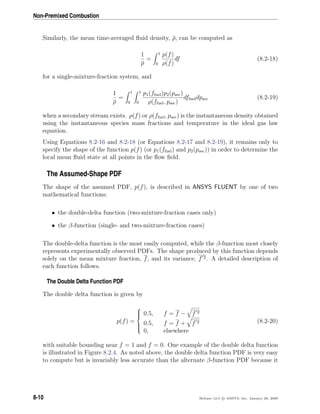
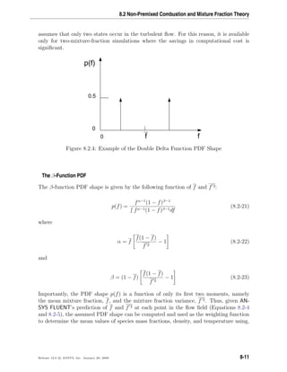
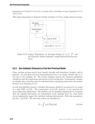
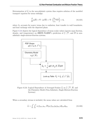
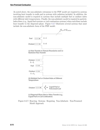
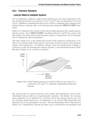
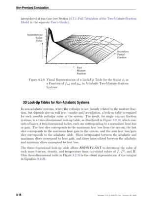
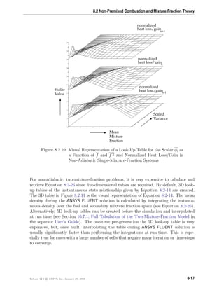
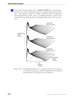
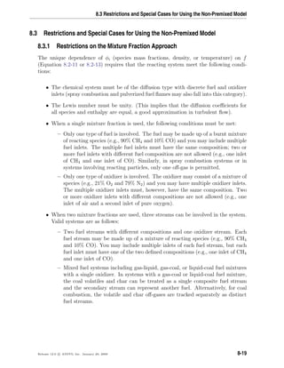
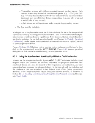
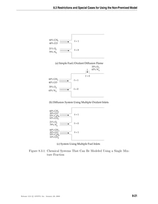
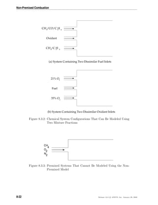
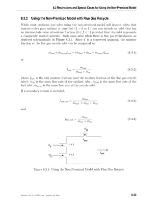
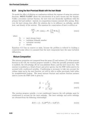
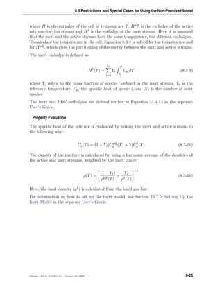
![Non-Premixed Combustion
8.4 The Laminar Flamelet Models Theory
Information about the flamelet models are presented in the following sections:
• Section 8.4.1: Restrictions and Assumptions
• Section 8.4.2: The Flamelet Concept
• Section 8.4.3: Flamelet Generation
• Section 8.4.4: Flamelet Import
8.4.1 Restrictions and Assumptions
The following restrictions apply to all flamelet models in ANSYS FLUENT:
• Only a single mixture fraction can be modeled; two-mixture-fraction flamelet mod-
els are not allowed.
• The mixture fraction is assumed to follow the β-function PDF, and scalar dissipa-
tion fluctuations are ignored.
• Empirically-based streams cannot be used with the flamelet model.
8.4.2 The Flamelet Concept
Overview
The flamelet concept views the turbulent flame as an ensemble of thin, laminar, locally
one-dimensional flamelet structures embedded within the turbulent flow field [36, 267,
268] (see Figure 8.4.1).
A common laminar flame type used to represent a flamelet in a turbulent flow is the
counterflow diffusion flame. This geometry consists of opposed, axisymmetric fuel and
oxidizer jets. As the distance between the jets is decreased and/or the velocity of the
jets increased, the flame is strained and increasingly departs from chemical equilibrium
until it is eventually extinguished. The species mass fraction and temperature fields can
be measured in laminar counterflow diffusion flame experiments, or, most commonly,
calculated. For the latter, a self-similar solution exists, and the governing equations can
be simplified to one dimension along the axis of the fuel and oxidizer jets, where complex
chemistry calculations can be affordably performed.
8-26 Release 12.0 c ANSYS, Inc. January 29, 2009](https://image.slidesharecdn.com/flth-130501182911-phpapp02/85/Flth-302-320.jpg)
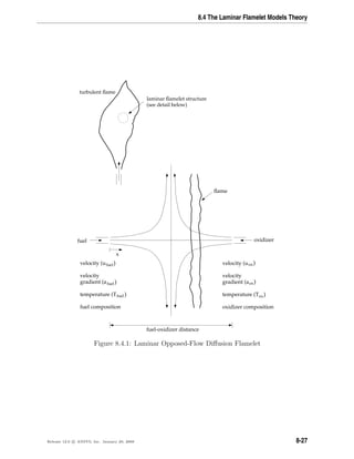
![Non-Premixed Combustion
In the laminar counterflow flame, the mixture fraction, f, (see Section 8.2.1: Definition
of the Mixture Fraction for definition) decreases monotonically from unity at the fuel
jet to zero at the oxidizer jet. If the species mass fraction and temperature along the
axis are mapped from physical space to mixture fraction space, they can be uniquely
described by two parameters: the mixture fraction and the strain rate (or, equivalently,
the scalar dissipation, χ, defined in Equation 8.4-2). Hence, the chemistry is reduced and
completely described by the two quantities, f and χ.
This reduction of the complex chemistry to two variables allows the flamelet calcula-
tions to be preprocessed, and stored in look-up tables. By preprocessing the chemistry,
computational costs are reduced considerably.
The balance equations, solution methods, and sample calculations of the counterflow
laminar diffusion flame can be found in several references. Comprehensive reviews and
analyses are presented in the works of Bray and Peters, and Dixon-Lewis [36, 72].
Strain Rate and Scalar Dissipation
A characteristic strain rate for a counterflow diffusion flamelet can be defined as as =
v/2d, where v is the relative speed of the fuel and oxidizer jets, and d is the distance
between the jet nozzles.
Instead of using the strain rate to quantify the departure from equilibrium, it is expedient
to use the scalar dissipation, denoted by χ. The scalar dissipation is defined as
χ = 2D| f|2
(8.4-1)
where D is a representative diffusion coefficient.
Note that the scalar dissipation, χ, varies along the axis of the flamelet. For the coun-
terflow geometry, the flamelet strain rate as can be related to the scalar dissipation at
the position where f is stoichiometric by [267]:
χst =
as exp −2[erfc−1
(2fst)]2
π
(8.4-2)
where
χst = scalar dissipation at f = fst
as = characteristic strain rate
fst = stoichiometric mixture fraction
erfc−1
= inverse complementary error function
8-28 Release 12.0 c ANSYS, Inc. January 29, 2009](https://image.slidesharecdn.com/flth-130501182911-phpapp02/85/Flth-304-320.jpg)
![8.4 The Laminar Flamelet Models Theory
Physically, as the flame is strained, the width of the reaction zone diminishes, and the
gradient of f at the stoichiometric position f = fst increases. The instantaneous stoi-
chiometric scalar dissipation, χst, is used as the essential non-equilibrium parameter. It
has the dimensions s−1
and may be interpreted as the inverse of a characteristic diffusion
time. In the limit χst → 0 the chemistry tends to equilibrium, and as χst increases due
to aerodynamic straining, the non-equilibrium increases. Local quenching of the flamelet
occurs when χst exceeds a critical value.
Embedding Laminar Flamelets in Turbulent Flames
A turbulent flame brush is modeled as an ensemble of discrete laminar flamelets. Since,
for adiabatic systems, the species mass fraction and temperature in the laminar flamelets
are completely parameterized by f and χst, density-weighted mean species mass fractions
and temperature in the turbulent flame can be determined from the PDF of f and χst as
φ = φ(f, χst)p(f, χst) df dχst (8.4-3)
where φ represents species mass fractions and temperature.
In ANSYS FLUENT, f and χst are assumed to be statistically independent, so the joint
PDF p(f, χst) can be simplified as pf (f)pχ(χst). A β PDF shape is assumed for pf , and
transport equations for f and f 2 are solved in ANSYS FLUENT to specify pf . Fluctu-
ations in χst are ignored so that the PDF of χ is a delta function: pχ = δ(χ − χ). The
first moment, namely the mean scalar dissipation, χst, is modeled in ANSYS FLUENT as
χst =
Cχ f 2
k
(8.4-4)
where Cχ is a constant with a default value of 2.
For LES, the mean scalar dissipation is modeled as
χst = Cχ
(µt + µ)
ρσt
| f|
2
(8.4-5)
To avoid the PDF convolutions at ANSYS FLUENT run-time, the integrations in Equa-
tion 8.4-3 are preprocessed and stored in look-up tables. For adiabatic flows, flamelet
tables have three dimensions: f, f 2 and χst.
For non-adiabatic steady laminar flamelets, the additional parameter of enthalpy is re-
quired. However, the computational cost of modeling steady flamelets over a range of
enthalpies is prohibitive, so some approximations are made. Heat gain/loss to the system
is assumed to have a negligible effect on the species mass fractions, and adiabatic mass
fractions are used [27, 240]. The temperature is then calculated from Equation 5.2-7
Release 12.0 c ANSYS, Inc. January 29, 2009 8-29](https://image.slidesharecdn.com/flth-130501182911-phpapp02/85/Flth-305-320.jpg)
![Non-Premixed Combustion
for a range of mean enthalpy gain/loss, H. Accordingly, mean temperature and density
PDF tables have an extra dimension of mean enthalpy. The approximation of constant
adiabatic species mass fractions is, however, not applied for the case corresponding to a
scalar dissipation of zero. Such a case is represented by the non-adiabatic equilibrium
solution. For χst = 0, the species mass fractions are computed as functions of f, f 2, and
H.
In ANSYS FLUENT, you can either generate your own flamelets, or import them as
flamelet files calculated with other stand-alone packages. Such stand-alone codes include
OPPDIF [210], CFX-RIF [15, 16, 272] and RUN-1DL [270]. ANSYS FLUENT can import
flamelet files in OPPDIF format or standard flamelet file format.
Instructions for generating and importing flamelets are provided in Section 8.4.3: Flamelet
Generation and Section 8.4.4: Flamelet Import.
8.4.3 Flamelet Generation
The laminar counterflow diffusion flame equations can be transformed from physical
space (with x as the independent variable) to mixture fraction space (with f as the
independent variable) [273]. In ANSYS FLUENT, a simplified set of the mixture fraction
space equations are solved [272]. Here, N equations are solved for the species mass
fractions, Yi,
ρ
∂Yi
∂t
=
1
2
ρχ
∂2
Yi
∂f2
+ Si (8.4-6)
and one equation for temperature:
ρ
∂T
∂t
=
1
2
ρχ
∂2
T
∂f2
−
1
cp i
HiSi +
1
2cp
ρχ
∂cp
∂f
+
i
cp,i
∂Yi
∂f
∂T
∂f
(8.4-7)
The notation in Equations 8.4-6 and 8.4-7 is as follows: Yi, T, ρ, and f are the ith species
mass fraction, temperature, density, and mixture fraction, respectively. cp,i and cp are
the ith species specific heat and mixture-averaged specific heat, respectively. Si is the
ith species reaction rate, and Hi is the specific enthalpy of the ith species.
The scalar dissipation, χ, must be modeled across the flamelet. An extension of Equa-
tion 8.4-2 to variable density is used [163]:
χ(f) =
as
4π
3( ρ∞/ρ + 1)
2
2 ρ∞/ρ + 1
exp −2[erfc−1
(2f)]2
(8.4-8)
where ρ∞ is the density of the oxidizer stream.
8-30 Release 12.0 c ANSYS, Inc. January 29, 2009](https://image.slidesharecdn.com/flth-130501182911-phpapp02/85/Flth-306-320.jpg)
![8.4 The Laminar Flamelet Models Theory
8.4.4 Flamelet Import
ANSYS FLUENT can import one or more flamelet files, convolute these flamelets with the
assumed-shape PDFs (see Equation 8.4-3), and construct look-up tables. The flamelet
files can be generated in ANSYS FLUENT, or with separate stand-alone computer codes.
Three types of flamelet files can be imported into ANSYS FLUENT: binary files generated
by the OPPDIF code [210], ASCII files generated by the CFX-RIF code [15, 16, 272], and
standard format files described in Section 16.7.4: Standard Flamelet Files in the separate
User’s Guide and in Peters and Rogg [270].
When flamelets are generated in physical space (such as with OPPDIF), the species and
temperature vary in one spatial dimension. The species and temperature must then be
mapped from physical space to mixture fraction space. If the diffusion coefficients of
all species are equal, a unique definition of the mixture fraction exists. However, with
differential diffusion, the mixture fraction can be defined in a number of ways.
ANSYS FLUENT provides four methods of computing the mixture fraction profile along
the laminar flamelet:
• Average of C and H: Following the work of Drake and Blint [77], the mixture
fraction is calculated as the mean value of fC and fH, where fC and fH are the
mixture fraction values based on the carbon and hydrogen elements.
• Hydrocarbon formula: Following the work of Bilger et al. [26], the mixture fraction
is calculated as
f =
b − box
bfuel − box
(8.4-9)
where
b = 2
YC
Mw,C
+ 0.5
YH
Mw,H
−
YO
Mw,O
(8.4-10)
YC, YH, and YO are the mass fractions of carbon, hydrogen, and oxygen atoms, and
Mw,C, Mw,H, and Mw,O are the molecular weights. box and bfuel are the values of b
at the oxidizer and fuel inlets.
• Nitrogen method: The mixture fraction is computed in terms of the mass fraction
of the nitrogen species:
f =
YN − YN,ox
YN,fuel − YN,ox
(8.4-11)
where YN is the elemental mass fraction of nitrogen along the flamelet, YN,ox is the
mass fraction of nitrogen at the oxidizer inlet, and YN,fuel is the mass fraction of
nitrogen at the fuel inlet.
Release 12.0 c ANSYS, Inc. January 29, 2009 8-31](https://image.slidesharecdn.com/flth-130501182911-phpapp02/85/Flth-307-320.jpg)
![Non-Premixed Combustion
• Read from a file (standard format files only): This option is for flamelets solved in
mixture fraction space. If you choose this method, ANSYS FLUENT will search for
the mixture fraction keyword Z, as specified in Peter and Roggs’s work [270], and
retrieve the data. If ANSYS FLUENT does not find mixture fraction data in the
flamelet file, it will instead use the hydrocarbon formula method described above.
The flamelet profiles in the multiple-flamelet data set should vary only in the strain rate
imposed; the species and the boundary conditions should be the same. In addition, it is
recommended that an extinguished flamelet is excluded from the multiple-flamelet data
set. The formats for multiple flamelets are as follows:
• OPPDIF format: The multiple-flamelet OPPDIF files should be produced using the
CNTN keyword in the OPPDIF script. Alternatively, you can use ANSYS FLUENT
to merge a number of single-flamelet OPPDIF files into a multiple-flamelet file.
• Standard format: If you have a set of standard format flamelet files, you can import
them all at the same time, and ANSYS FLUENT will merge them internally into a
multiple-flamelet file. When you import the set of flamelet files, ANSYS FLUENT
will search for and count the occurrences of the HEADER keyword to determine the
number of flamelets in the file.
• CFX-RIF format: A CFX-RIF flamelet file contains multiple flamelets at various
strains and the file should not be modified manually. Only one CFX-RIF flamelet
file should be imported.
For either type of file, ANSYS FLUENT will determine the number of flamelet profiles
and sort them in ascending strain-rate order. For flamelets generated in physical space,
you can select one of the four methods available for the calculation of mixture fraction.
The scalar dissipation will be calculated from the strain rate using Equation 8.4-2.
8.5 The Steady Laminar Flamelet Model Theory
The steady laminar flamelet approach models a turbulent flame brush as an ensemble of
discrete, steady laminar flames, called flamelets. The individual flamelets are assumed
to have the same structure as laminar flames in simple configurations, and are obtained
by experiments or calculations. Using detailed chemical mechanisms, ANSYS FLUENT
can calculate laminar opposed-flow diffusion flamelets for non-premixed combustion. The
laminar flamelets are then embedded in a turbulent flame using statistical PDF methods.
The advantage of the laminar flamelet approach is that realistic chemical kinetic effects
can be incorporated into turbulent flames. The chemistry can then be preprocessed
and tabulated, offering tremendous computational savings. However, the steady laminar
flamelet model is limited to modeling combustion with relatively fast chemistry. The
flame is assumed to respond instantaneously to the aerodynamic strain, and thus the
8-32 Release 12.0 c ANSYS, Inc. January 29, 2009](https://image.slidesharecdn.com/flth-130501182911-phpapp02/85/Flth-308-320.jpg)
![8.5 The Steady Laminar Flamelet Model Theory
where the slope si is defined as,
si =
vi+1 − vi
fi+1 − fi
(8.5-4)
In Equations 8.5-3 and 8.5-4, s is a user specified Maximum Change in Slope Ratio (default
of 0.5), smax (smin) are the maximum (minimum) slopes over all grid points, and fi is
the mixture fraction value of grid point i.
The refined flamelet is reconverged, and the refinement process is repeated until no further
grid points are added by Equations 8.5-2 and 8.5-3, or the user specified Maximum Number
of Grid Points in Flamelet (default of 64) is exceeded.
8.5.4 Non-Adiabatic Steady Laminar Flamelets
For non-adiabatic steady flamelets, ANSYS FLUENT follows the approach of [27, 240]
and assumes that flamelet species profiles are unaffected by heat loss/gain from the
flamelet. No special non-adiabatic flamelet profiles need to be generated, avoiding a very
cumbersome preprocessing step. In addition, the compatibility of ANSYS FLUENT with
external steady flamelet generation packages (e.g., OPPDIF, CFX-RIF, RUN-1DL) is
retained. The disadvantage to this model is that the effect of the heat losses on the
species mass fractions is not taken into account. Also, the effect of the heat loss on the
extinction limits is not taken into account.
After flamelet generation, the flamelet profiles are convoluted with the assumed-shape
PDFs as in Equation 8.4-3, and then tabulated for look-up in ANSYS FLUENT. The
non-adiabatic PDF tables have the following dimensions:
T(f, f 2, H, χ)
Yi(f, f 2, H) for χ = 0 (i.e., equilibrium solution)
Yi(f, f 2, χ) for χ = 0
ρ(f, f 2, H, χ)
During the ANSYS FLUENT solution, the equations for the mean mixture fraction, mix-
ture fraction variance, and mean enthalpy are solved. The scalar dissipation field is
calculated from the turbulence field and the mixture fraction variance (Equation 8.4-4).
The mean values of cell temperature, density, and species mass fraction are obtained
from the PDF look-up table.
Release 12.0 c ANSYS, Inc. January 29, 2009 8-35](https://image.slidesharecdn.com/flth-130501182911-phpapp02/85/Flth-311-320.jpg)
![Non-Premixed Combustion
8.6 The Unsteady Laminar Flamelet Model Theory
The steady laminar flamelet model, described in Sections 8.4 and 8.5, models local chem-
ical non-equilibrium due to the straining effect of turbulence. In many combustors the
strain is small at the outlet and the steady flamelet model predicts all species, including
slow-forming species like NOx, to be near equilibrium, which is often inaccurate. The
cause of this inaccuracy is the disparity between the flamelet time-scale, which is the
inverse of the scalar dissipation, and the slow-forming species time-scale, which is the
residence time since the species started accumulating after mixing in the combustor.
The unsteady laminar flamelet model in ANSYS FLUENT can predict slow-forming species,
such as gaseous pollutants or product yields in liquid reactors, more accurately than
the steady laminar flamelet model. Computationally expensive chemical kinetics are
reduced to one dimension and the model is significantly faster than the laminar-finite-
rate, EDC or PDF Transport models where kinetics are calculated in two or three di-
mensions. There are two variants of the unsteady laminar flamelet model, namely an
Eulerian unsteady flamelet model (described in Section 8.6.1: The Eulerian Unsteady
Laminar Flamelet Model) and a diesel unsteady flamelet model for predicting combus-
tion in compression-ignition engines (described in Section 8.6.2: The Diesel Unsteady
Laminar Flamelet Model).
Information pertaining strictly to the unsteady flamelet model is presented in the follow-
ing sections:
• Section 8.6.1: The Eulerian Unsteady Laminar Flamelet Model
• Section 8.6.2: The Diesel Unsteady Laminar Flamelet Model
8.6.1 The Eulerian Unsteady Laminar Flamelet Model
The Eulerian unsteady laminar flamelet model can be used to predict slow-forming inter-
mediate and product species which are not in chemical equilibrium. Typical examples of
slow-forming species are gas-phase pollutants like NOx, and product compounds in liq-
uid reactors. By reducing the chemistry computation to one dimension, detailed kinetics
with multiple species and stiff reactions can be economically simulated in complex 3D
geometries.
The model, following the work of Barths et al. [16], postprocesses an unsteady marker
probability equation on a steady-state, converged flow field. In ANSYS FLUENT, the
steady flow solution must be computed with the steady laminar flamelet model (see
Section 8.5: The Steady Laminar Flamelet Model Theory). Since the unsteady flamelet
equations are postprocessed on a steady-state, steady flamelet solution, the effect of the
unsteady flamelet species on the flow-field are neglected.
8-36 Release 12.0 c ANSYS, Inc. January 29, 2009](https://image.slidesharecdn.com/flth-130501182911-phpapp02/85/Flth-312-320.jpg)
![8.6 The Unsteady Laminar Flamelet Model Theory
The effect of high Sc is to decrease mixing at the smallest (micro) scales and increase
the mixture fraction variance, which is modeled with the Turbulent Mixer Model [11].
Three transport equations are solved for the inertial-convective (f 2
ic ), viscous-convective
(f 2
vc), and viscous-diffusive (f 2
vd) subranges of the turbulent scalar spectrum,
∂
∂t
ρf 2
ic + · ρvf 2
ic = ·
µt
σt
f 2
ic + C1µt f
2
− C2ρ
k
f 2
ic (8.6-7)
∂
∂t
ρf 2
vc + · ρvf 2
vc = ·
µt
σt
f 2
vc + C2ρ
k
f 2
ic − C3ρ
ν
f 2
vc (8.6-8)
∂
∂t
ρf 2
vd + · ρvf 2
vd = ·
µt
σt
f 2
vd + C3ρ
ν
f 2
vc − C4 +
C5
Sc
f 2
vd (8.6-9)
where the constants C1 through C5 have values of 2, 1.86, 0.058, 0.303, and 17050,
respectively. The total mixture fraction variance is the sum of f 2
ic , f 2
vc and f 2
vd.
In Equation 8.6-9, the cell Schmidt number, Sc, is calculated as Sc = µ/ρD where µ
is the viscosity, ρ the density, and D the mass diffusivity as defined for the pdf-mixture
material.
8.6.2 The Diesel Unsteady Laminar Flamelet Model
In diesel engines, fuel sprayed into the cylinder evaporates, mixes with the surrounding
gases, and then auto-ignites as compression raises the temperature and pressure. The
diesel unsteady laminar flamelet model, based on the work of Pitsch et al. and Barths
et al. [272, 15], models the chemistry in a single, one-dimensional laminar flamelet. By
reducing the costly chemical kinetic calculation to 1D, substantial savings in run-time
can be achieved over the laminar-finite-rate, EDC or PDF Transport models.
The flamelet species and energy equations (Equations 8.4-6 and 8.4-7) are solved simul-
taneously with the flow. The flamelet equations are advanced for a fractional step using
properties from the flow, and then the flow is advanced for the same fractional time-step
using properties from the flamelet.
The initial flamelet condition at the start of the diesel simulation is a mixed-but-unburnt
distribution. For the flamelet fractional time-step, the volume-averaged scalar dissipation
and pressure, as well as the fuel and oxidizer temperatures, are passed from the flow solver
to the flamelet solver. To account for temperature rise during compression, the flamelet
energy equation (Equation 8.4-7) has an additional term on the right-hand side as
˙q =
1
cp
∂p
∂t
(8.6-10)
Release 12.0 c ANSYS, Inc. January 29, 2009 8-39](https://image.slidesharecdn.com/flth-130501182911-phpapp02/85/Flth-315-320.jpg)

![9.2 Zimont Turbulent Flame Closure Theory
9.2 Zimont Turbulent Flame Closure Theory
The turbulent premixed combustion model, based on work by Zimont et al. [390, 391,
393], involves the solution of a transport equation for the reaction progress variable. The
closure of this equation is based on the definition of the turbulent flame speed.
Information in this section is provided in the following sections:
• Section 9.2.1: Propagation of the Flame Front
• Section 9.2.2: Turbulent Flame Speed
9.2.1 Propagation of the Flame Front
In many industrial premixed systems, combustion takes place in a thin flame sheet.
As the flame front moves, combustion of unburnt reactants occurs, converting unburnt
premixed reactants to burnt products. The premixed combustion model thus considers
the reacting flow field to be divided into regions of burnt and unburnt species, separated
by the flame sheet.
The flame front propagation is modeled by solving a transport equation for the density-
weighted mean reaction progress variable, denoted by c:
∂
∂t
(ρc) + · (ρvc) = ·
µt
Sct
c + ρSc (9.2-1)
where
c = mean reaction progress variable
Sct = turbulent Schmidt number
Sc = reaction progress source term (s−1
)
The progress variable is defined as a normalized sum of the product species,
c =
n
i=1
Yi
n
i=1
Yi,eq
(9.2-2)
where
n = number of products
Yi = mass fraction of product species i
Yi,eq = equilibrium mass fraction of product species i
Release 12.0 c ANSYS, Inc. January 29, 2009 9-3](https://image.slidesharecdn.com/flth-130501182911-phpapp02/85/Flth-319-320.jpg)
![Premixed Combustion
Based on this definition, c = 0 where the mixture is unburnt and c = 1 where the mixture
is burnt:
• c = 0: unburnt mixture
• c = 1: burnt mixture
The value of c is defined as a boundary condition at all flow inlets. It is usually specified
as either 0 (unburnt) or 1 (burnt).
The mean reaction rate in Equation 9.2-1 is modeled as [391]
ρSc = ρuUt| c| (9.2-3)
where
ρu = density of unburnt mixture
Ut = turbulent flame speed
Many other models for turbulent flame speed exist [36], and can be specified using user-
defined functions. More information about user-defined functions can be found in the
separate UDF Manual.
9.2.2 Turbulent Flame Speed
The key to the premixed combustion model is the prediction of Ut, the turbulent flame
speed normal to the mean surface of the flame. The turbulent flame speed is influenced
by the following:
• laminar flame speed, which is, in turn, determined by the fuel concentration, tem-
perature, and molecular diffusion properties, as well as the detailed chemical kinet-
ics
• flame front wrinkling and stretching by large eddies, and flame thickening by small
eddies
In ANSYS FLUENT, the Zimont turbulent flame speed closure is computed using a model
for wrinkled and thickened flame fronts [391]:
Ut = A(u )3/4
U
1/2
l α−1/4 1/4
t (9.2-4)
= Au
τt
τc
1/4
(9.2-5)
9-4 Release 12.0 c ANSYS, Inc. January 29, 2009](https://image.slidesharecdn.com/flth-130501182911-phpapp02/85/Flth-320-320.jpg)
![9.2 Zimont Turbulent Flame Closure Theory
where
A = model constant
u = RMS (root-mean-square) velocity (m/s)
Ul = laminar flame speed (m/s)
α = k/ρcp = molecular heat transfer coefficient of unburnt
mixture (thermal diffusivity) (m2
/s)
t = turbulence length scale (m)
τt = t/u = turbulence time scale (s)
τc = α/U2
l = chemical time scale (s)
The turbulence length scale, t, is computed from
t = CD
(u )3
(9.2-6)
where is the turbulence dissipation rate.
The model is based on the assumption of equilibrium small-scale turbulence inside the
laminar flame, resulting in a turbulent flame speed expression that is purely in terms
of the large-scale turbulent parameters. The default value of 0.52 for A is recom-
mended [391], and is suitable for most premixed flames. The default value of 0.37 for CD
should also be suitable for most premixed flames.
The model is strictly applicable when the smallest turbulent eddies in the flow (the
Kolmogorov scales) are smaller than the flame thickness, and penetrate into the flame
zone. This is called the thin reaction zone combustion region, and can be quantified by
Karlovitz numbers, Ka, greater than unity. Ka is defined as
Ka =
tl
tη
=
v2
η
U2
l
(9.2-7)
where
tl = characteristic flame time scale
tη = smallest (Kolmogorov) turbulence time scale
vη = (ν )1/4
= Kolmogorov velocity
ν = kinematic viscosity
Lastly, the model is valid for premixed systems where the flame brush width increases in
time, as occurs in most industrial combustors. Flames that propagate for a long period
of time equilibrate to a constant flame width, which cannot be captured in this model.
Release 12.0 c ANSYS, Inc. January 29, 2009 9-5](https://image.slidesharecdn.com/flth-130501182911-phpapp02/85/Flth-321-320.jpg)
![Premixed Combustion
Turbulent Flame Speed for LES
For simulations that use the LES turbulence model, the Reynolds-averaged quantities in
the turbulent flame speed expression (Equation 9.2-4) are replaced by their equivalent
subgrid quantities. In particular, the large eddy length scale t is modeled as
t = Cs∆ (9.2-8)
where Cs is the Smagorinsky constant and ∆ is the cell characteristic length.
The RMS velocity in Equation 9.2-4 is replaced by the subgrid velocity fluctuation,
calculated as
u = tτ−1
sgs (9.2-9)
where τ−1
sgs is the subgrid scale mixing rate (inverse of the subgrid scale time scale), given
in Equation 7.1-28.
Laminar Flame Speed
The laminar flame speed (Ul in Equation 9.2.1) can be specified as constant, or as a
user-defined function. A third option appears for non-adiabatic premixed and partially-
premixed flames and is based on the correlation proposed by Meghalchi and Keck [227],
Ul = Ul,ref
Tu
Tu,ref
γ
pu
pu,ref
β
(9.2-10)
In Equation 9.2-10, Tu and pu are the unburnt reactant temperature and pressure ahead
of the flame, Tu,ref = 298K and pu,ref = 1atm.
The reference laminar flame speed, Ul,ref , is calculated from
Ul,ref = C1 + C2(φ − C3)2
(9.2-11)
where φ is the equivalence ratio ahead of the flame front, and C1, C2 and C3 are fuel-
specific constants. The exponents γ and β are calculated from,
γ = 2.18 − 0.8(φ − 1)
β = −0.16 + 0.22(φ − 1)
(9.2-12)
The Meghalchi-Keck laminar flame speeds are available for fuel-air mixtures of methane,
methanol, propane, iso-octane and indolene fuels.
9-6 Release 12.0 c ANSYS, Inc. January 29, 2009](https://image.slidesharecdn.com/flth-130501182911-phpapp02/85/Flth-322-320.jpg)
![9.2 Zimont Turbulent Flame Closure Theory
Unburnt Density and Thermal Diffusivity
The unburnt density (ρu in Equation 9.2.1) and unburnt thermal diffusivity (α in Equa-
tion 9.2-5) are specified constants that are set in the Materials dialog box. However, for
compressible cases, such as in-cylinder combustion, these can change significantly in time
and/or space. When the ideal gas model is selected for density, the unburnt density and
thermal diffusivity are calculated as volume averages ahead of the flame front.
Flame Stretch Effect
Since industrial low-emission combustors often operate near lean blow-off, flame stretch-
ing will have a significant effect on the mean turbulent heat release intensity. To take
this flame stretching into account, the source term for the progress variable (ρSc in Equa-
tion 9.2-1) is multiplied by a stretch factor, G [393]. This stretch factor represents the
probability that the stretching will not quench the flame; if there is no stretching (G = 1),
the probability that the flame will be unquenched is 100%.
The stretch factor, G, is obtained by integrating the log-normal distribution of the tur-
bulence dissipation rate, :
G =
1
2
erfc
−
1
2σ
ln
cr
+
σ
2
(9.2-13)
where erfc is the complementary error function, and σ and cr are defined below.
σ is the standard deviation of the distribution of :
σ = µstr ln
L
η
(9.2-14)
where µstr is the stretch factor coefficient for dissipation pulsation, L is the turbulent
integral length scale, and η is the Kolmogorov micro-scale. The default value of 0.26 for
µstr (measured in turbulent non-reacting flows) is recommended by [391], and is suitable
for most premixed flames.
cr is the turbulence dissipation rate at the critical rate of strain [391]:
cr = 15νg2
cr (9.2-15)
Release 12.0 c ANSYS, Inc. January 29, 2009 9-7](https://image.slidesharecdn.com/flth-130501182911-phpapp02/85/Flth-323-320.jpg)
![Premixed Combustion
By default, gcr is set to a very high value (1 × 10⁸
) so no flame stretching occurs. To
include flame stretching effects, the critical rate of strain gcr should be adjusted based on
experimental data for the burner. Numerical models can suggest a range of physically
plausible values [391], or an appropriate value can be determined from experimental data.
A reasonable model for the critical rate of strain gcr is
gcr =
BU2
l
α
(9.2-16)
where B is a constant (typically 0.5) and α is the unburnt thermal diffusivity. Equa-
tion 9.2-16 can be implemented in ANSYS FLUENTusing a property user-defined function.
More information about user-defined functions can be found in the separate UDF Manual.
Gradient Diffusion
Volume expansion at the flame front can cause counter-gradient diffusion. This effect
becomes more pronounced when the ratio of the reactant density to the product den-
sity is large, and the turbulence intensity is small. It can be quantified by the ratio
(ρu/ρb)(Ul/I), where ρu, ρb, Ul, and I are the unburnt and burnt densities, laminar flame
speed, and turbulence intensity, respectively. Values of this ratio greater than one indi-
cate a tendency for counter-gradient diffusion, and the premixed combustion model may
be inappropriate. Recent arguments for the validity of the turbulent-flame-speed model
in such regimes can be found in Zimont et al. [392].
Wall Damping
High turbulent kinetic energy levels at the walls in some problems can cause an unphysical
acceleration of the flame along the wall. In reality, radical quenching close to walls
decreases reaction rates and thus the flame speed, but is not included in the model. To
approximate this effect, ANSYS FLUENT includes a constant multiplier for the turbulent
flame speed, αw, which modifies the flame speed in the vicinity of wall boundaries:
Ut = αwA
τt
τc
1/4
(9.2-17)
The default for this constant is 1 which does not change the flame speed. Values of αw
larger than 1 increase the flame speed, while values less than 1 decrease the flame speed
in the cells next to the wall boundary.
9-8 Release 12.0 c ANSYS, Inc. January 29, 2009](https://image.slidesharecdn.com/flth-130501182911-phpapp02/85/Flth-324-320.jpg)
![9.3 Extended Coherent Flamelet Model Theory
ANSYS FLUENT will solve the transport equation for the reaction progress variable c
(Equation 9.2-1), computing the source term, ρSc, based on the theory outlined above:
ρSc = AGρuI3/4
[Ul(λlp)]1/2
[α(λlp)]−1/4 1/4
t | c| (9.2-18)
= AGρuI
τt
τc(λlp)
1/4
| c| (9.2-19)
9.3 Extended Coherent Flamelet Model Theory
The Extended Coherent Flamelet Model (ECFM) [274] is a more refined premixed com-
bustion model than the Zimont Turbulent Flame Closure. It has theoretically greater
accuracy, but is less robust and requires greater computational effort to converge.
Information in this section is provided in the following sections:
• Section 9.3.1: Closure for ECFM Source Terms
• Section 9.3.2: Turbulent Flame Speed in ECFM
The ECFM model solves an additional equation for the flame area density, denoted Σ,
which is ultimately used to model the mean reaction rate in Equation 9.2-1. The model
assumes that the smallest turbulence length scales (Kolmogorov eddies) are larger than
the laminar flame thickness, so the effect of turbulence is to wrinkle the laminar flame
sheet, however the internal laminar flame profile is not distorted. The increased surface
area of the flame results in increased net fuel consumption and an increased flame speed.
The range of applicability of the ECFM model is illustrated on the Borghi diagram in
Figure 9.3.1, where the wrinkled flamelets regime is indicated below the Da = 1 line.
Typical Internal Combustion (IC) engines typically operate in this wrinkled flamelet
range.
An expression for the transport of the net flame area per unit volume, or flame area
density, Σ, can be derived based on these assumptions [44]:
∂Σ
∂t
+ · (vΣ) = ·
µt
Sct
Σ
ρ
+ (P1 + P2 + P3) Σ − D (9.3-1)
Release 12.0 c ANSYS, Inc. January 29, 2009 9-9](https://image.slidesharecdn.com/flth-130501182911-phpapp02/85/Flth-325-320.jpg)
![Premixed Combustion
E
T
2222222222222222222222
2222222222222222222222
d
d
d
d
d
d
d
d
d
d
d
d
d
d
d
d
IC
Engines
87
96
lt/δl
1 10 100 1000
u /Ul
1
10
Laminar
Combustion
Wrinkled
Flamelets
Thickened
Flamelets
Thickened
Flames
Da = 1
Ka = 1
Ret = 1
Ka = 100
Figure 9.3.1: Borghi diagram for turbulent combustion
where
Σ = mean flame area density
Sct = turbulent Schmidt number
µt = turbulent viscosity
ρ = density
P1 = Source due to turbulence interaction
P2 = Source due to dilatation in the flame
P3 = Source due to expansion of burned gas
D = Dissipation of flame area
Equation 9.3-1 requires closure terms for the production and destruction terms for flame
area density. Several families of closure terms have been put forth in the literature [274].
ANSYS FLUENT uses the closure described in the following section.
9-10 Release 12.0 c ANSYS, Inc. January 29, 2009](https://image.slidesharecdn.com/flth-130501182911-phpapp02/85/Flth-326-320.jpg)
![9.3 Extended Coherent Flamelet Model Theory
9.3.1 Closure for ECFM Source Terms
P1 represents the production of flame area density by turbulent flame stretching, and is
modeled as
P1 = α1Kt = α1
k
[(1 − α0) + α0ΓK] (9.3-2)
where Kt is a turbulent time scale and α1 is a constant with a default value of 1.6. The
constant α0 (default of 1) is a user-specified linear blending between the Intermediate
Turbulent Net Flame Stretch (ITNFS) term, ΓK, for low turbulence levels at α0 = 1, and
a straightforward turbulent time scale source when α0 = 0 for high turbulence levels.
The ITNFS term, ΓK, can be specified either as a constant or calculated as a function
of the two parameters u /Ul and lt/δ0
L, where u is the turbulent velocity fluctuation, Ul
is the laminar flame speed, lt is the integral turbulent length scale and δ0
L is the laminar
flame thickness.
The expression for ΓK is given by:
log10(ΓK) = −
1
(s + 0.4)
exp (−(s + 0.4)) + (1 − exp (−(s + 0.4))) σ1
u
Ul
s − 0.11
(9.3-3)
where s is defined as
s = log10
lt
δ0
l
(9.3-4)
and σ1 is
σ1
u
Ul
=
2
3
1 −
1
2
exp
−
u
Ul
1
3
(9.3-5)
The ITNFS term, ΓK, is sensitive to the laminar flame thickness. ANSYS FLUENT
provides several options for the calculation of this quantity:
• Constant (user-specified) value
• Meneveau Flame Thickness [223]
The laminar flame thickness is calculated as
δ0
l =
2α
Ul
(9.3-6)
Release 12.0 c ANSYS, Inc. January 29, 2009 9-11](https://image.slidesharecdn.com/flth-130501182911-phpapp02/85/Flth-327-320.jpg)
![Premixed Combustion
where α is the local unburnt thermal diffusivity.
• Poinsot Flame Thickness [274]
The flame thickness is evaluated as in Equation 9.3-6 but an additional term, Γp is
added to ΓK. Γp is calculated as
Γp = −
3
2
ltUl
δlu
log
1
1 − pq
(9.3-7)
where
pq = −1
2
(1 + tanh (b3
/|b|))
b = [log10 (u /Ul) − gl] /0.04s
gl = (0.7 + es
) e−s
+ (1 + e−s
) (1 + 0.36s)
s = log10 (ltUl/α)
• Blint Correction Flame Thickness [30]
This includes a correction due to rapid expansion of the gas:
δ0
l = 2
Tb
Tu
0.7
α
Ul
(9.3-8)
where Tu is the unburned temperature, and Tb denotes the burned temperature.
The term P2 in Equation 9.3-1 models the influence of dilatation on the production of
flame area density. The term is given by
P2 = α2
2
3
· (ρu) (9.3-9)
where the constant α2 has a default of 1.
The term P3 models the effect of thermal expansion of the burned gas on the flame area
density, and is given by
P3 = α3
ρu
ρb
Ul
1 − c
c
Σ (9.3-10)
where α3 is 1 by default.
The flame area destruction term D is modeled as
D = βUl
Σ2
1 − c
(9.3-11)
9-12 Release 12.0 c ANSYS, Inc. January 29, 2009](https://image.slidesharecdn.com/flth-130501182911-phpapp02/85/Flth-328-320.jpg)
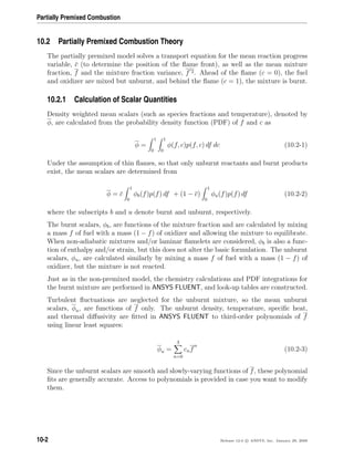
![10.2 Partially Premixed Combustion Theory
10.2.2 Laminar Flame Speed
The premixed models require the laminar flame speed (see Equation 9.2-4), which de-
pends strongly on the composition, temperature, and pressure of the unburnt mixture.
For adiabatic perfectly premixed systems as in Chapter 9: Premixed Combustion, the
reactant stream has one composition, and the laminar flame speed is constant through-
out the domain. However, in partially premixed systems, the laminar flame speed will
change as the reactant composition (equivalence ratio) changes, and this must be taken
into account.
Accurate laminar flame speeds are difficult to determine analytically, and are usually
measured from experiments or computed from 1D simulations. ANSYS FLUENT uses
fitted curves obtained from numerical simulations of the laminar flame speed [114]. These
curves were determined for hydrogen (H2), methane (CH4), acetylene (C2H2), ethylene
(C2H4), ethane (C2H6), and propane (C3H8) fuels. They are valid for inlet compositions
ranging from the lean limit through unity equivalence ratio (stoichiometric), for unburnt
temperatures from 298 K to 800 K, and for pressures from 1 bar to 40 bars.
ANSYS FLUENT fits these curves to a piecewise-linear polynomial. Mixtures leaner than
the lean limit or richer than the rich limit will not burn, and have zero flame speed. The
required inputs are values for the laminar flame speed at ten mixture fraction (f) points.
The first (minimum) and last (maximum) f inputs are the flammability limits of the
mixture and the laminar flame speed is zero outside these value.
i These flame speed fits are accurate for air mixtures with pure fuels of H2,
CH4, C2H2, C2H4, C2H6, and C3H8. If an oxidizer other than air or a
different fuel is used, or if the unburnt temperature or pressure is outside
the range of validity, then the curve fits will be incorrect. Although AN-
SYS FLUENT defaults to a methane-air mixture, the laminar flame speed
polynomial and the rich and lean limits are most likely incorrect for your
specified fuel/oxidizer and unburnt temperature/pressure conditions. The
laminar flame speed polynomial should be determined from other sources,
such as measurements from the relevant literature or detailed 1D simula-
tions, and then input into ANSYS FLUENT.
Release 12.0 c ANSYS, Inc. January 29, 2009 10-3](https://image.slidesharecdn.com/flth-130501182911-phpapp02/85/Flth-333-320.jpg)

![Composition PDF Transport
11.2 Composition PDF Transport Theory
Turbulent combustion is governed by the reacting Navier-Stokes equations. While this
equation set is accurate, its direct solution (where all turbulent scales are resolved) is far
too expensive for practical turbulent flows. In Chapter 7: Species Transport and Finite-
Rate Chemistry, the species equations are Reynolds-averaged, which leads to unknown
terms for the turbulent scalar flux and the mean reaction rate. The turbulent scalar flux
is modeled in ANSYS FLUENT by gradient diffusion, treating turbulent convection as
enhanced diffusion. The mean reaction rate can be modeled with the Laminar, Eddy-
Dissipation or EDC Finite-Rate chemistry models. Since the reaction rate is invariably
highly non-linear, modeling the mean reaction rate in a turbulent flow is difficult and
prone to error.
An alternative to Reynolds-averaging the species and energy equations is to derive a
transport equation for their single-point, joint probability density function (PDF). This
PDF, denoted by P, can be considered to represent the fraction of the time that the
fluid spends at each species, temperature and pressure state. P has N + 2 dimensions
for the N species, temperature and pressure spaces. From the PDF, any single-point
thermo-chemical moment (e.g., mean or RMS temperature, mean reaction rate) can be
calculated. The composition PDF transport equation is derived from the Navier-Stokes
equations as [276]:
∂
∂t
(ρP) +
∂
∂xi
(ρuiP) +
∂
∂ψk
(ρSkP) = −
∂
∂xi
ρ ui |ψ P +
∂
∂ψk
ρ
1
ρ
∂Ji,k
∂xi
ψ P
(11.2-1)
where
P = Favre joint PDF of composition
ρ = mean fluid density
ui = Favre mean fluid velocity vector
Sk = reaction rate for specie k
ψ = composition space vector
ui = fluid velocity fluctuation vector
Ji,k = molecular diffusion flux vector
The notation of . . . denotes expectations, and A|B is the conditional probability of
event A, given that event B occurs.
11-2 Release 12.0 c ANSYS, Inc. January 29, 2009](https://image.slidesharecdn.com/flth-130501182911-phpapp02/85/Flth-336-320.jpg)
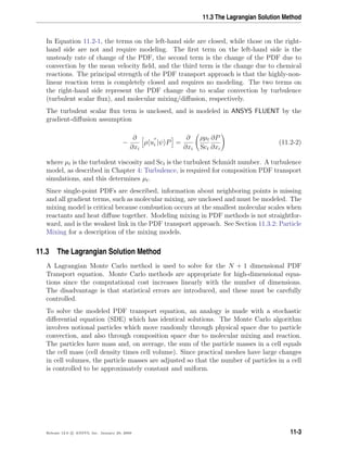
![Composition PDF Transport
The processes of convection, diffusion, and reaction are treated in fractional steps as
described in the sections that follow. For information on the fractional step method,
refer to [45].
Information about this method is described in the following sections:
• Section 11.3.1: Particle Convection
• Section 11.3.2: Particle Mixing
• Section 11.3.3: Particle Reaction
• Section 11.3.4: The ISAT Algorithm
11.3.1 Particle Convection
A spatially second-order-accurate Lagrangian method is used in ANSYS FLUENT, con-
sisting of two steps. At the first convection step, particles are advanced to a new position
x
1/2
i = x0
i +
1
2
u0
i ∆t (11.3-1)
where
xi = particle position vector
ui = Favre mean fluid-velocity vector at the particle position
∆t = particle time step
For unsteady flows, the particle time step is the physical time step. For steady-state
flows, local time steps are calculated for each cell as
∆t = min(∆tconv, ∆tdiff, ∆tmix) (11.3-2)
where
∆tconv = convection number × ∆x / (cell fluid velocity)
∆tdiff = diffusion number × (∆x)2
/ (cell turbulent diffusivity)
∆tmix = mixing number × turbulent time scale
∆x = characteristic cell length = volume1/D
where D is the problem dimension
After the first convection step, all other sub-processes, including diffusion and reaction
are treated. Finally, the second convection step is calculated as
x1
i = x
1/2
i + ∆t u
1/2
i −
1
2
u0
i +
1
ρSct
∂µt
∂xi
+ ξi
2µt
ρ∆tSct
(11.3-3)
where
11-4 Release 12.0 c ANSYS, Inc. January 29, 2009](https://image.slidesharecdn.com/flth-130501182911-phpapp02/85/Flth-338-320.jpg)
![11.3 The Lagrangian Solution Method
ρ = mean cell fluid density
ui = mean fluid-velocity vector at the particle position
µt = turbulent viscosity
Sct = turbulent Schmidt number
ξi = standardized normal random vector
11.3.2 Particle Mixing
Molecular mixing of species and heat must be modeled and is usually the source of the
largest modeling error in the PDF transport approach. ANSYS FLUENT provides three
models for molecular diffusion: the Modified Curl model [147, 250], the IEM model
(which is sometimes called the LSME model) [75] and the EMST model [340].
The Modified Curl Model
For the Modified Curl model, a few particle pairs are selected at random from all the
particles in a cell, and their individual compositions are moved toward their mean com-
position. For the special case of equal particle mass, the number of particle pairs selected
is calculated as
Npair =
1.5CφN∆t
τt
(11.3-4)
where
N = total number of particles in the cell
Cφ = mixing constant (default = 2)
τt = turbulent time scale (for the k- model this is k/ )
The algorithm in [250] is used for the general case of variable particle mass.
For each particle pair, a uniform random number ξ is selected and each particle’s com-
position φ is moved toward the pair’s mean composition by a factor proportional to ξ:
φ1
i = (1 − ξ)φ0
i + ξ
(φ0
i mi + φ0
j mj)
(mi + mj)
φ1
j = (1 − ξ)φ0
j + ξ
(φ0
i mi + φ0
j mj)
(mi + mj)
(11.3-5)
where φi and φj are the composition vectors of particles i and j, and mi and mj are the
masses of particles i and j.
Release 12.0 c ANSYS, Inc. January 29, 2009 11-5](https://image.slidesharecdn.com/flth-130501182911-phpapp02/85/Flth-339-320.jpg)
![Composition PDF Transport
The IEM Model
For the Interaction by Exchange with the Mean (IEM) model, the composition of all
particles in a cell are moved a small distance toward the mean composition:
φ1
= φ0
− 1 − e−0.5Cφ/τt
φ0
− ˜φ (11.3-6)
where φ0
is the composition before mixing, φ1
is the composition after mixing, and ˜φ is
the Favre mean-composition vector at the particle’s location.
The EMST Model
Physically, mixing occurs between fluid particles that are adjacent to each other. The
Modified Curl and IEM mixing models take no account of this localness, which can be a
source of error. The Euclidean Minimum Spanning Tree (EMST) model mixes particle
pairs that are close to each other in composition space. Since scalar fields are locally
smooth, particles that are close in composition space are likely to be close in physical
space. The particle pairing is determined by a Euclidean Minimum Spanning Tree, which
is the minimum length of the set of edges connecting one particle to at least one other
particle. The EMST mixing model is more accurate than the Modified Curl and IEM
mixing models, but incurs a slightly greater computational expense. Details on the EMST
model can be found in reference [340].
Liquid Reactions
Reactions in liquids often occur at low turbulence levels (small Re), among reactants
with low diffusivities (large Sc). For such flows, the mixing constant default of Cφ = 2
overestimates the mixing rate. The Liquid Micro-Mixing option interpolates Cφ from
model turbulence [278] and scalar [103] spectra.
11.3.3 Particle Reaction
The particle composition vector is represented as
φ = (Y1, Y2, . . . , YN , T, p) (11.3-7)
where Yk is the kth specie mass fraction, T is the temperature and p the pressure.
For the reaction fractional step, the reaction source term is integrated as
φ1
= φ0
+
∆t
0
Sdt (11.3-8)
11-6 Release 12.0 c ANSYS, Inc. January 29, 2009](https://image.slidesharecdn.com/flth-130501182911-phpapp02/85/Flth-340-320.jpg)
![11.3 The Lagrangian Solution Method
where S is the chemical source term. Most realistic chemical mechanisms consist of
tens of species and hundreds of reactions. Typically, a reaction does not occur until
an ignition temperature is reached, but then proceeds very quickly until reactants are
consumed. Hence, some reactions have very fast time scales, in the order of 10−10
s, while
others have much slower time scales, on the order of 1 s. This time-scale disparity results
in numerical stiffness, which means that extensive computational work is required to
integrate the chemical source term in Equation 11.3-8. In ANSYS FLUENT, the reaction
step (i.e., the calculation of φ1
) can be performed either by Direct Integration or by
In-Situ Adaptive Tabulation (ISAT), as described in the following paragraphs.
A typical steady-state PDF transport simulation in ANSYS FLUENT may have 50000
cells, with 20 particles per cell, and requires 1000 iterations to converge. Hence, at least
109
stiff ODE integrations are required. Since each integration typically takes tens or
hundreds of milliseconds, on average, the direct integration of the chemistry is extremely
CPU-demanding.
For a given reaction mechanism, Equation 11.3-8 may be considered as a mapping. With
an initial composition vector φ0
, the final state φ1
depends only on φ0
and the mapping
time ∆t. In theory, if a table could be built before the simulation, covering all realizable
φ0
states and time steps, the integrations could be avoided by table look-ups. In practice,
this a priori tabulation is not feasible since a full table in N + 3 dimensions (N species,
temperature, pressure and time-step) is required. To illustrate this, consider a structured
table with M points in each dimension. The required table size is MN+3
, and for a
conservative estimate of M = 10 discretization points and N = 7 species, the table
would contain 1010
entries.
On closer examination, the full storage of the entire realizable space is very wasteful
because most regions are never accessed. For example, it would be unrealistic to find a
composition of YOH = 1 and T = 300K in a real combustor. In fact, for steady-state, 3D
laminar simulations, the chemistry can be parameterized by the spatial position vector.
Thus, mappings must lie on a three dimensional manifold within the N + 3 dimensional
composition space. It is, hence, sufficient to tabulate only this accessed region of the
composition space.
The accessed region, however, depends on the particular chemical mechanism, molecular
transport properties, flow geometry, and boundary conditions. For this reason, the ac-
cessed region is not known before the simulation and the table cannot be preprocessed.
Instead, the table must be built during the simulation, and this is referred to as in-situ
tabulation. ANSYS FLUENT employs ISAT [277] to dynamically tabulate the chemistry
mappings and accelerate the time to solution. ISAT is a method to tabulate the accessed
composition space region “on the fly” (in-situ) with error control (adaptive tabulation).
When ISAT is used correctly, accelerations of two to three orders of magnitude are typical.
However, it is important to understand how ISAT works in order to use it optimally.
Release 12.0 c ANSYS, Inc. January 29, 2009 11-7](https://image.slidesharecdn.com/flth-130501182911-phpapp02/85/Flth-341-320.jpg)
![11.4 The Eulerian Solution Method
The ISAT algorithm is summarized as follows:
1. The ISAT table is queried for every composition vector during the reaction step.
2. For each query φ0
q the table is traversed to identify a leaf whose composition φ0
is
close to φ0
q.
3. If the query composition φ0
q lies within the EOA of the leaf, then the mapping φ1
q
is retrieved using interpolation by Equation 11.3-9. Otherwise, Direct Integration
(DI) is performed and the error between the DI and the linear interpolation is
measured.
4. If the error is less than the tolerance, then the ellipsoid of accuracy is grown and
the DI result is returned. Otherwise, a new table entry is added.
At the start of the simulation, most operations are adds and grows. Later, as more of
the composition space is tabulated, retrieves become frequent. Since adds and grows are
very slow whereas retrieves are relatively quick, initial ANSYS FLUENT iterations are
slow but accelerate as the table is built.
11.4 The Eulerian Solution Method
The Lagrangian solution method solves the composition PDF transport equation by
stochastically tracking Lagrangian particles through the domain. It is computationally
expensive since a large number of particles are required to represent the PDF, and a
large number of iterations are necessary to reduce statistical errors and explicitly convect
the particles through the domain. The Eulerian PDF transport model overcomes these
limitations by assuming a shape for the PDF, which allows Eulerian transport equations
to be derived. Stochastic errors are eliminated and the transport equations are solved
implicitly, which is computationally economical. The multi-dimensional PDF shape is
assumed as a product of delta functions. As with the Lagrangian PDF model, the
highly non-linear chemical source term is closed. However, the turbulent scalar flux and
molecular mixing terms must be modeled, and are closed with the gradient diffusion and
the IEM models, respectively.
The composition PDF of Ns + 1 dimension (Ns species and enthalpy) is represented as a
collection of Ne delta functions (or modes). This presumed PDF has the following form:
P(ψ; x, t) =
Ne
n=1
pn(x, t)
Ns
k=1
δ[ψk− φk n (x, t)] (11.4-1)
where pn is the probability in each mode, φk n is the conditional mean composition
of specie k in the nth mode, ψk is the composition space variable of specie k, and δ(. . .)
is the delta function.
Release 12.0 c ANSYS, Inc. January 29, 2009 11-9](https://image.slidesharecdn.com/flth-130501182911-phpapp02/85/Flth-343-320.jpg)
![Composition PDF Transport
The Eulerian PDF transport equations are derived by substituting Equation 11.4-1 into
the closed composition PDF transport equation (Equation 11.2-1 with Equations 11.2-2
and 11.3-6). The unknown terms, pn and φk n, are determined by forcing lower
moments of this transported PDF to match the RANS lower moment transport equations,
using the Direct Quadrature Method of Moments (DQMOM) approach [103, 218]. The
resulting transport equations are:
• Probability (magnitude of the nth delta function):
∂ρpn
∂t
+
∂
∂xi
(ρuipn) = (ρΓ pn) (11.4-2)
• Probability weighted conditional mean of composition k:
∂ρsk,n
∂t
+
∂
∂xi
(ρuisk,n) = (ρΓ sk,n) + ρ(Mk,n + Sk,n + Ck,n) (11.4-3)
where pn is the probability of the nth mode, and sk,n = pn φk n is the kth specie
probability weighted conditional mean composition of the nth mode. Γ = µl + µt/Sct
is the effective turbulent diffusivity. The terms Mk,n, Sk,n and Ck,n represent mixing,
reaction and correction terms respectively. Note that only Ne − 1 probability equations
are solved and the Nth probability is calculated as one minus the sum of the Ne − 1
solved probabilities.
Reaction
The reaction source term Sk,n in Equation 11.4-3 for the kth composition and the nth
mode is calculated as,
Sk,n = pnS( φk n)k (11.4-4)
where S()k is the net reaction rate for the kth component.
Mixing
The micro-mixing term Mk,n is modeled with the IEM mixing model:
Mk,n =
Cφ
τ
( φk n −ψk) (11.4-5)
where τ is the turbulence time-scale and Cφ is the mixing constant.
Hence, for the two-mode DQMOM-IEM model, the mixing terms for component k are,
11-10 Release 12.0 c ANSYS, Inc. January 29, 2009](https://image.slidesharecdn.com/flth-130501182911-phpapp02/85/Flth-344-320.jpg)
![11.4 The Eulerian Solution Method
Mk,1 =
Cφ
τ
(p1sk,2 − p2sk,1)
Mk,2 =
Cφ
τ
(p2sk,1 − p1sk,2) (11.4-6)
The default value of Cφ is 2, which is appropriate for gas-phase combustion. For reactions
in liquids, where the diffusivities are much smaller than gases, the Liquid Micro-Mixing
option interpolates Cφ from model turbulence [278] and scalar [103] spectra.
Correction
Using assumptions to ensure realizability and boundedness, the correction terms Ck,n in
Equation 11.4-3 for the kth composition are determined from the linear system,
Ne
n=1
φk mk−1
n Ck,n =
Ne
n=1
(mk − 1) φk mk−2
n pnck,n (11.4-7)
where mk are the non-negative integer lower moments (1..Ne) for each component k.
Note that the condition of the matrix decreases with increasing mk, which reduces the
stability of higher mode simulations.
The dissipation term ck,n in Equation 11.4-7 is calculated as,
ck,n = Γ ( φk n) · ( φk n) (11.4-8)
For the two-mode DQMOM-IEM model, the correction terms for the kth component are,
Ck,1 =
Γ
φk 1 − φk 2
p1( φk 1)2
+ p2( φk 2)2
Ck,2 = −Ck,1 (11.4-9)
Calculation of Composition Mean and Variance
The mean composition (specie k or energy) is calculated as,
φk =
Ne
n=1
sk,n (11.4-10)
and its variance is calculated as
φ 2
k = (
Ne
n=1
sk,n φk n) − φk
2
(11.4-11)
Release 12.0 c ANSYS, Inc. January 29, 2009 11-11](https://image.slidesharecdn.com/flth-130501182911-phpapp02/85/Flth-345-320.jpg)

![Chapter 12. Engine Ignition
This chapter discusses the theory behind the engine ignition models available in ANSYS
FLUENT. Information can be found in the following sections.
• Section 12.1: Spark Model
• Section 12.2: Autoignition Models
• Section 12.3: Crevice Model
For information about using these ignition models, see Chapter 20: Modeling Engine
Ignition in the separate User’s Guide.
12.1 Spark Model
The spark model in ANSYS FLUENT will be described in the context of the premixed tur-
bulent combustion model. For information about using this model, see Section 20.1: Spark
Model in the separate User’s Guide. Information regarding the theory behind this model
is detailed in the following sections:
• Section 12.1.1: Overview and Limitations
• Section 12.1.2: Spark Model Theory
12.1.1 Overview and Limitations
Initiation of combustion at a desired time and location in a combustion chamber can be
accomplished by sending a high voltage across two narrowly separated wires, creating
a spark. The spark event in typical engines happens very quickly relative to the main
combustion in the engine. The physical description of this simple event is very involved
and complex, making it difficult to accurately model the spark in the context of a multi-
dimensional engine simulation. Additionally, the energy from the spark event is several
orders of magnitude less than the chemical energy release from the fuel. Despite the
amount of research devoted to spark ignition physics and ignition devices, the ignition
of a mixture at a point in the domain is more dependent on the local composition than
on the spark energy (see Heywood [128]). Thus, for situations in which ANSYS FLUENT
is utilized for combustion engine modeling, including internal combustion engines, the
Release 12.0 c ANSYS, Inc. January 29, 2009 12-1](https://image.slidesharecdn.com/flth-130501182911-phpapp02/85/Flth-347-320.jpg)
![Engine Ignition
spark event does not need to be modeled in great detail, but simply as the initiation of
combustion over a duration, which you will set.
Since spark ignition is inherently transient, the spark model is only available in the
transient solver. Additionally, the spark model requires chemical reactions to be solved.
The spark model is available for all of the combustion models, however, it may be most
applicable to the premixed and partially premixed combustion models.
The Spark Model used in ANSYS FLUENT is based on a one-dimensional analysis by Li-
patnikov [203]. The model is sensitive to perturbations and can be subject to instabilities
when used in multi-dimensional simulations. The instabilities are inherent to the model
and can be dependent on the mesh, especially near the beginning of the spark event
when the model reduces diffusion to simulate the initial laminar spark kernel growth.
The instability is susceptible to numerical errors which are increased when the mesh is
not aligned with the flame propagation. As the spark kernel grows and the model allows
turbulent mixing to occur, the effect of the instability decreases.
12.1.2 Spark Model Theory
The spark model in ANSYS FLUENT is based on the work done by Lipatnikov [203] and
extended to other combustion models. The derivation of the model can be done in the
context of the Zimont premixed combustion model.
Zimont Premixed Flame Model
The transport equation for the mean reaction progress variable, c, is given by Equa-
tion 12.1-1
∂ρc
∂t
+ · (ρvc) = · (Dt c) + ρuUt| c| (12.1-1)
where Dt is the turbulent diffusivity, ρu is the density of the unburned mixture and Ut
is the turbulent flame speed. Since the spark is often very small compared to the mesh
size of the model and is often laminar in nature, the Zimont model is modified such that
∂ρc
∂t
+ · (ρvc) = · ((κ + Dtt) c) + ρuUt| c| (12.1-2)
where κ is the laminar thermal diffusivity and the effective diffusivity Dtt is given by
Dtt =
Dt 1 − exp −ttd
τ
if ttd ≥ 0
Dt if ttd 0
(12.1-3)
where is ttd = t−tig and tig denotes the time at which the spark is initiated. Additionally,
τ is an effective diffusion time, which you can set.
12-2 Release 12.0 c ANSYS, Inc. January 29, 2009](https://image.slidesharecdn.com/flth-130501182911-phpapp02/85/Flth-348-320.jpg)
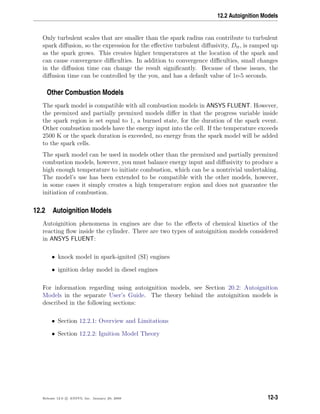
![12.2 Autoignition Models
The autoignition models in general require adjustment of parameters to reproduce engine
data and are likely to require tuning to improve accuracy. Once the model is calibrated to
a particular engine configuration, then different engine speeds and loads can be reasonably
well represented. Detailed chemical kinetics may be more applicable over a wider range of
conditions, though are more expensive to solve. The single equation autoignition models
are appropriate for the situation where geometric fidelity or resolution of particular flow
details is more important than chemical effects on the simulation.
12.2.2 Ignition Model Theory
Both the knock and the ignition delay models are treated similarly in ANSYS FLUENT,
in that they share the same infrastructure. These models belong to the family of sin-
gle equation autoignition models and use correlations to account for complex chemical
kinetics. They differ from the eight step reaction models, such as Halstead’s “Shell”
model [121], in that only a single transport equation is solved. The source term in the
transport equation is typically not stiff, thus making the equation relatively inexpensive
to solve.
This approach is appropriate for large simulations where geometric accuracy is more im-
portant than fully resolved chemical kinetics. The model can be used on less resolved
meshes to explore a range of designs quickly, and to obtain trends before utilizing more
expensive and presumably more accurate chemical mechanisms in multidimensional sim-
ulations.
Transport of Ignition Species
Autoignition is modeled using the transport equation for an Ignition Species, Yig, which
is given by
∂ρYig
∂t
+ · (ρvYig) = ·
µt
Sct
Yig + ρSig (12.2-1)
where Yig is a “mass fraction” of a passive species representing radicals which form when
the fuel in the domain breaks down. Sct is the turbulent Schmidt number. The term Sig
is the source term for the ignition species which has a form
Sig =
t
t=t0
dt
τig
where t0 corresponds to the time at which fuel is introduced into the domain. The τig
term is a correlation of ignition delay with the units of time. Ignition has occurred when
the ignition species reaches a value of 1 in the domain. It is assumed that all the radical
species represented by Yig diffuse at the same rate as the mean flow.
Release 12.0 c ANSYS, Inc. January 29, 2009 12-5](https://image.slidesharecdn.com/flth-130501182911-phpapp02/85/Flth-351-320.jpg)
![Engine Ignition
Note that the source term for these radical species is treated differently for knock and
ignition delay. Furthermore, the form of the correlation of ignition delay differs between
the two models. Details of how the source term is treated are covered in the following
sections.
Knock Modeling
When modeling knock or ignition delay, chemical energy in the fuel is released when
the ignition species reaches a value of 1 in the domain. For the knock model, two
correlations are built into ANSYS FLUENT. One is given by Douaud [76], while the other
is a generalized model which reproduces several correlations, given by Heywood [128].
Modeling of the Source Term
In order to model knock in a physically realistic manner, the source term is accumu-
lated under appropriate conditions in a cell. Consider the one dimensional flame in
Figure 12.2.1. Here, the flame is propagating from left to right, and the temperature is
relatively low in front of the flame and high behind the flame. In this figure, Tb and Tu
represent the temperatures at the burned and unburned states, respectively. The ignition
species accumulates only when there is fuel. In the premixed model, the fuel is defined
as fuel = 1 − c, where c is the progress variable. If the progress variable has a value of
zero, the mixture is considered unburned. If the progress variable is 1, then the mixture
is considered burned.
E
T
¤
¦ E
X
T
Tb
Tu
fuel = 0
Sig = 0
fuel 0
Sig 0
Figure 12.2.1: Flame Front Showing Accumulation of Source Terms for the
Knock Model
When the ignition species reaches a value of 1 in the domain, knock has occurred at that
point. The value of the ignition species can exceed unity. In fact, values well above that
can be obtained in a short time. The ignition species will continue to accumulate until
there is no more fuel present.
12-6 Release 12.0 c ANSYS, Inc. January 29, 2009](https://image.slidesharecdn.com/flth-130501182911-phpapp02/85/Flth-352-320.jpg)
![12.2 Autoignition Models
Correlations
An extensively tested correlation for knock in SI engines is given by Douaud and Eyzat [76]:
τ = 0.01768
ON
100
3.402
p−1.7
exp
3800
T
(12.2-2)
where ON is the octane number of the fuel, p is the absolute pressure in atmospheres
and T is the temperature in Kelvin.
A generalized expression for τ is also available which can reproduce many existing Ar-
rhenius correlations. The form of the correlation is
τ = A
ON
100
a
pb
Tc
RPMd
Φd
exp
−Ea
RT
(12.2-3)
where A is the pre-exponential (with units in seconds), RPM is the engine speed in cycles
per minute and Φ is the fuel/air equivalence ratio.
Energy Release
Once ignition has occurred in the domain, the knock event is modeled by releasing the
remaining fuel energy with a single-step Arrhenius reaction. An additional source term,
which burns the remaining fuel in that cell, is added to the rate term in the premixed
model. The reaction rate is given by
˙ω = A0 exp
−Ea
RT
(12.2-4)
where A0 = 8.6 × 10⁹
, and Ea = −15078. These values are chosen to reflect single-step
reaction rates appropriate for propane as described in Amsden [4]. The rate at which the
fuel is consumed is limited such that a completely unburned cell will burn during three of
the current time steps. Limiting the reaction rate is done purely for numerical stability.
Ignition Delay Modeling
When modeling ignition delay in diesel engines, chemical reactions are allowed to occur
when the ignition species reaches a value of 1 in the domain. For the ignition delay model,
two correlations are built into ANSYS FLUENT, one given by Hardenburg and Hase [125]
and the other, a generalized model which reproduces several Arrhenius correlations from
the literature.
Release 12.0 c ANSYS, Inc. January 29, 2009 12-7](https://image.slidesharecdn.com/flth-130501182911-phpapp02/85/Flth-353-320.jpg)
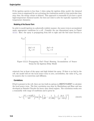
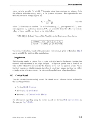
![Engine Ignition
12.3.1 Overview
The crevice model implemented in ANSYS FLUENT is a zero-dimensional ring-flow model
based on the model outlined in Namazian and Heywood [245] and Roberts and Matthews [295].
The model is geared toward in-cylinder specific flows, and more specifically, direct-
injection (DI) diesel engines, and thus is available only for time-dependent simulations.
The model takes mass, momentum, and energy from cells adjoining two boundaries and
accounts for the storage of mass in the volumes of the crevices in the piston. Detailed
geometric information regarding the ring and piston—typically a ring pack around the
bore of an engine—is necessary to use the crevice model. An example representation is
shown in Figures 12.3.1–12.3.3.
Cylinder
wall
Piston to bore
clearance
Land length
Ring spacing
p
0
p
6
1
2
3
1: Top gap
2: Middle gap
3: Bottom gap
Figure 12.3.1: Crevice Model Geometry (Piston)
Wr
Tr
Figure 12.3.2: Crevice Model Geometry (Ring)
12-10 Release 12.0 c ANSYS, Inc. January 29, 2009](https://image.slidesharecdn.com/flth-130501182911-phpapp02/85/Flth-356-320.jpg)
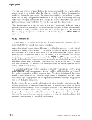

![Pollutant Formation
where YHCN, YNH3 , YN2O, and YNO are mass fractions of HCN, NH3, N2O, and NO in
the gas phase, and D is the effective diffusion coefficient. The source terms SHCN, SNH3 ,
SN2O, and SNO are to be determined next for different NOx mechanisms.
13.1.3 Thermal NOx Formation
The formation of thermal NOx is determined by a set of highly temperature-dependent
chemical reactions known as the extended Zeldovich mechanism. The principal reactions
governing the formation of thermal NOx from molecular nitrogen are as follows:
O + N2 N + NO (13.1-5)
N + O2 O + NO (13.1-6)
A third reaction has been shown to contribute to the formation of thermal NOx, partic-
ularly at near-stoichiometric conditions and in fuel-rich mixtures:
N + OH H + NO (13.1-7)
Thermal NOx Reaction Rates
The rate constants for these reactions have been measured in numerous experimental
studies [29, 102, 236], and the data obtained from these studies have been critically
evaluated by Baulch et al. [18] and Hanson and Salimian [124]. The expressions for the
rate coefficients for Equations 13.1-5–13.1-7 used in the NOx model are given below.
These were selected based on the evaluation of Hanson and Salimian [124].
kf,1 = 1.8 × 10⁸
e−38370/T
kr,1 = 3.8 × 10⁷
e−425/T
kf,2 = 1.8 × 10⁴
Te−4680/T
kr,2 = 3.81 × 10³
Te−20820/T
kf,3 = 7.1 × 10⁷
e−450/T
kr,3 = 1.7 × 10⁸
e−24560/T
In the above expressions, kf,1, kf,2, and kf,3 are the rate constants for the forward reactions
13.1-5–13.1-7, respectively, and kr,1, kr,2, and kr,3 are the corresponding reverse rate
constants. All of these rate constants have units of m3
/gmol-s.
The net rate of formation of NO via Reactions 13.1-5–13.1-7 is given by
d[NO]
dt
= kf,1[O][N2] + kf,2[N][O2] + kf,3[N][OH] − kr,1[NO][N] − kr,2[NO][O] − kr,3[NO][H]
(13.1-8)
where all concentrations have units of gmol/m3
.
To calculate the formation rates of NO and N, the concentrations of O, H, and OH are
required.
13-4 Release 12.0 c ANSYS, Inc. January 29, 2009](https://image.slidesharecdn.com/flth-130501182911-phpapp02/85/Flth-364-320.jpg)
![13.1 NOx Formation
The Quasi-Steady Assumption for [N]
The rate of formation of NOx is significant only at high temperatures (greater than
1800 K) because fixation of nitrogen requires the breaking of the strong N2 triple bond
(dissociation energy of 941 kJ/gmol). This effect is represented by the high activation
energy of reaction 13.1-5, which makes it the rate-limiting step of the extended Zeldovich
mechanism. However, the activation energy for oxidation of N atoms is small. When
there is sufficient oxygen, as in a fuel-lean flame, the rate of consumption of free nitrogen
atoms becomes equal to the rate of its formation and therefore a quasi-steady state can
be established. This assumption is valid for most combustion cases except in extremely
fuel-rich combustion conditions. Hence the NO formation rate becomes
d[NO]
dt
= 2kf,1[O][N2]
1 − kr,1kr,2[NO]2
kf,1[N2]kf,2[O2]
1 + kr,1[NO]
kf,2[O2]+kf,3[OH]
(gmol/m3
-s) (13.1-9)
Thermal NOx Temperature Sensitivity
From Equation 13.1-9 it is clear that the rate of formation of NO will increase with
increasing oxygen concentration. It also appears that thermal NO formation should be
highly dependent on temperature but independent of fuel type. In fact, based on the
limiting rate described by kf,1, the thermal NOx production rate doubles for every 90 K
temperature increase beyond 2200 K.
Decoupled Thermal NOx Calculations
To solve Equation 13.1-9, the concentration of O atoms and the free radical OH will
be required, in addition to the concentration of stable species (i.e., O2, N2). Following
the suggestion by Zeldovich, the thermal NOx formation mechanism can be decoupled
from the main combustion process, by assuming equilibrium values of temperature, sta-
ble species, O atoms, and OH radicals. However, radical concentrations, O atoms in
particular, are observed to be more abundant than their equilibrium levels. The effect of
partial equilibrium O atoms on NOx formation rate has been investigated [232] during
laminar methane-air combustion. The results of these investigations indicate that the
level of NOx emission can be underpredicted by as much as 28% in the flame zone, when
assuming equilibrium O-atom concentrations.
Release 12.0 c ANSYS, Inc. January 29, 2009 13-5](https://image.slidesharecdn.com/flth-130501182911-phpapp02/85/Flth-365-320.jpg)
![Pollutant Formation
Approaches for Determining O Radical Concentration
There has been little detailed study of radical concentration in industrial turbulent flames,
but work [79] has demonstrated the existence of this phenomenon in turbulent diffusion
flames. Presently, there is no definitive conclusion as to the effect of partial equilibrium
on NOx formation rates in turbulent flames. Peters and Donnerhack [269] suggest that
partial equilibrium radicals can account for no more than a 25% increase in thermal NOx
and that fluid dynamics has the dominant effect on NOx formation rate. Bilger et al. [25]
suggest that in turbulent diffusion flames, the effect of O atom overshoot on the NOx
formation rate is very important.
To overcome this possible inaccuracy, one approach would be to couple the extended Zel-
dovich mechanism with a detailed hydrocarbon combustion mechanism involving many
reactions, species, and steps. This approach has been used previously for research pur-
poses [229]. However, long computer processing time has made the method economically
unattractive and its extension to turbulent flows difficult.
To determine the O radical concentration, ANSYS FLUENT uses one of three approaches—
the equilibrium approach, the partial equilibrium approach, and the predicted concen-
tration approach—in recognition of the ongoing controversy discussed above.
Method 1: Equilibrium Approach
The kinetics of the thermal NOx formation rate is much slower than the main hydro-
carbon oxidation rate, and so most of the thermal NOx is formed after completion of
combustion. Therefore, the thermal NOx formation process can often be decoupled from
the main combustion reaction mechanism and the NOx formation rate can be calculated
by assuming equilibration of the combustion reactions. Using this approach, the calcu-
lation of the thermal NOx formation rate is considerably simplified. The assumption of
equilibrium can be justified by a reduction in the importance of radical overshoots at
higher flame temperature [78]. According to Westenberg [377], the equilibrium O-atom
concentration can be obtained from the expression
[O] = kp[O2]1/2
(13.1-10)
With kp included, this expression becomes
[O] = 3.97 × 10⁵
T−1/2
[O2]1/2
e−31090/T
gmol/m3
(13.1-11)
where T is in Kelvin.
13-6 Release 12.0 c ANSYS, Inc. January 29, 2009](https://image.slidesharecdn.com/flth-130501182911-phpapp02/85/Flth-366-320.jpg)
![13.1 NOx Formation
Method 2: Partial Equilibrium Approach
An improvement to method 1 can be made by accounting for third-body reactions in the
O2 dissociation-recombination process:
O2 + M O + O + M (13.1-12)
Equation 13.1-11 is then replaced by the following expression [367]:
[O] = 36.64T1/2
[O2]1/2
e−27123/T
gmol/m3
(13.1-13)
which generally leads to a higher partial O-atom concentration.
Method 3: Predicted O Approach
When the O-atom concentration is well predicted using an advanced chemistry model
(such as the flamelet submodel of the non-premixed model), [O] can be taken simply
from the local O-species mass fraction.
Approaches for Determining OH Radical Concentration
ANSYS FLUENT uses one of three approaches to determine the OH radical concentration:
the exclusion of OH from the thermal NOx calculation approach, the partial equilibrium
approach, and the use of the predicted OH concentration approach.
Method 1: Exclusion of OH Approach
In this approach, the third reaction in the extended Zeldovich mechanism (Equation 13.1-7)
is assumed to be negligible through the following observation:
k2[O2]eq k3[OH]eq
This assumption is justified for lean fuel conditions and is a reasonable assumption for
most cases.
Method 2: Partial Equilibrium Approach
In this approach, the concentration of OH in the third reaction in the extended Zeldovich
mechanism (Equation 13.1-7) is given by [19, 376]
[OH] = 2.129 × 10²
T−0.57
e−4595/T
[O]1/2
[H2O]1/2
gmol/m3
(13.1-14)
Release 12.0 c ANSYS, Inc. January 29, 2009 13-7](https://image.slidesharecdn.com/flth-130501182911-phpapp02/85/Flth-367-320.jpg)
![Pollutant Formation
Method 3: Predicted OH Approach
As in the predicted O approach, when the OH radical concentration is well predicted using
an advanced chemistry model such as the flamelet model, [OH] can be taken directly from
the local OH species mass fraction.
Summary
To summarize, thermal NOx formation rate is predicted by Equation 13.1-9. The
O-atom concentration needed in Equation 13.1-9 is computed using Equation 13.1-11
for the equilibrium assumption, using Equation 13.1-13 for a partial equilibrium assump-
tion, or using the local O-species mass fraction. You will make the choice during problem
setup. In terms of the transport equation for NO (Equation 13.1-1), the NO source term
due to thermal NOx mechanisms is
Sthermal,NO = Mw,NO
d[NO]
dt
(13.1-15)
where Mw,NO is the molecular weight of NO (kg/gmol), and d[NO]/dt is computed from
Equation 13.1-9.
13.1.4 Prompt NOx Formation
It is known that during combustion of hydrocarbon fuels, the NOx formation rate can
exceed that produced from direct oxidation of nitrogen molecules (i.e., thermal NOx).
Prompt NOx Combustion Environments
The presence of a second mechanism leading to NOx formation was first identified by
Fenimore [91] and was termed “prompt NOx”. There is good evidence that prompt NOx
can be formed in a significant quantity in some combustion environments, such as in low-
temperature, fuel-rich conditions and where residence times are short. Surface burners,
staged combustion systems, and gas turbines can create such conditions [13].
At present the prompt NOx contribution to total NOx from stationary combustors is
small. However, as NOx emissions are reduced to very low levels by employing new
strategies (burner design or furnace geometry modification), the relative importance of
the prompt NOx can be expected to increase.
13-8 Release 12.0 c ANSYS, Inc. January 29, 2009](https://image.slidesharecdn.com/flth-130501182911-phpapp02/85/Flth-368-320.jpg)
![13.1 NOx Formation
Prompt NOx Mechanism
Prompt NOx is most prevalent in rich flames. The actual formation involves a complex
series of reactions and many possible intermediate species. The route now accepted is as
follows:
CH + N2 HCN + N (13.1-16)
N + O2 NO + O (13.1-17)
HCN + OH CN + H2O (13.1-18)
CN + O2 NO + CO (13.1-19)
A number of species resulting from fuel fragmentation have been suggested as the source
of prompt NOx in hydrocarbon flames (e.g., CH, CH2, C, C2H), but the major contribu-
tion is from CH (Equation 13.1-16) and CH2, via
CH2 + N2 HCN + NH (13.1-20)
The products of these reactions could lead to formation of amines and cyano compounds
that subsequently react to form NO by reactions similar to those occurring in oxidation
of fuel nitrogen, for example:
HCN + N N2 + ... (13.1-21)
Prompt NOx Formation Factors
Prompt NOx formation is proportional to the number of carbon atoms present per unit
volume and is independent of the parent hydrocarbon identity. The quantity of HCN
formed increases with the concentration of hydrocarbon radicals, which in turn increases
with equivalence ratio. As the equivalence ratio increases, prompt NOx production in-
creases at first, then passes a peak, and finally decreases due to a deficiency in oxygen.
Primary Reaction
Reaction 13.1-16 is of primary importance. In recent studies [304], comparison of proba-
bility density distributions for the location of the peak NOx with those obtained for the
peak CH have shown close correspondence, indicating that the majority of the NOx at the
flame base is prompt NOx formed by the CH reaction. Assuming that Reaction 13.1-16
controls the prompt NOx formation rate,
d[NO]
dt
= k0[CH][N2] (13.1-22)
Release 12.0 c ANSYS, Inc. January 29, 2009 13-9](https://image.slidesharecdn.com/flth-130501182911-phpapp02/85/Flth-369-320.jpg)
![Pollutant Formation
Modeling Strategy
There are, however, uncertainties about the rate data for the above reaction. From Reac-
tions 13.1-16–13.1-20, it can be concluded that the prediction of prompt NOx formation
within the flame requires coupling of the NOx kinetics to an actual hydrocarbon com-
bustion mechanism. Hydrocarbon combustion mechanisms involve many steps and, as
mentioned previously, are extremely complex and costly to compute. In the present NOx
model, a global kinetic parameter derived by De Soete [69] is used. De Soete compared
the experimental values of total NOx formation rate with the rate of formation calculated
by numerical integration of the empirical overall reaction rates of NOx and N2 formation.
He showed that overall prompt formation rate can be predicted from the expression
d[NO]
dt
= (overall prompt NOx formation rate) − (overall prompt N2 formation rate)
(13.1-23)
In the early stages of the flame, where prompt NOx is formed under fuel-rich conditions,
the O concentration is high and the N radical almost exclusively forms NOx rather than
nitrogen. Therefore, the prompt NOx formation rate will be approximately equal to the
overall prompt NOx formation rate:
d[NO]
dt
= kpr[O2]a
[N2][FUEL]e−Ea/RT
(13.1-24)
For C2H4 (ethylene)-air flames,
kpr = 1.2 × 10⁷
(RT/p)a+1
; Ea = 251151 J/gmol
where a is the oxygen reaction order, R is the universal gas constant, and p is pressure
(all in SI units). The rate of prompt NOx formation is found to be of the first order with
respect to nitrogen and fuel concentration, but the oxygen reaction order, a, depends on
experimental conditions.
13-10 Release 12.0 c ANSYS, Inc. January 29, 2009](https://image.slidesharecdn.com/flth-130501182911-phpapp02/85/Flth-370-320.jpg)
![13.1 NOx Formation
Rate for Most Hydrocarbon Fuels
Equation 13.1-24 was tested against the experimental data obtained by Backmier et
al. [9] for different mixture strengths and fuel types. The predicted results indicated that
the model performance declined significantly under fuel-rich conditions and for higher
hydrocarbon fuels. To reduce this error and predict the prompt NOx adequately in
all conditions, the De Soete model was modified using the available experimental data.
A correction factor, f, was developed, which incorporates the effect of fuel type, i.e.,
number of carbon atoms, and air-to-fuel ratio for gaseous aliphatic hydrocarbons. Equa-
tion 13.1-24 now becomes
d[NO]
dt
= fkpr[O2]a
[N2][FUEL]e−Ea/RT
(13.1-25)
so that the source term due to prompt NOx mechanism is
Sprompt,NO = Mw,NO
d[NO]
dt
(13.1-26)
In the above equations,
f = 4.75 + 0.0819 n − 23.2φ + 32φ2
− 12.2φ3
(13.1-27)
kpr = 6.4 × 10⁶
(RT/p)a+1
; Ea = 303474.125 J/gmol
n is the number of carbon atoms per molecule for the hydrocarbon fuel, and φ is the
equivalence ratio. The correction factor is a curve fit for experimental data, valid for
aliphatic alkane hydrocarbon fuels (CnH2n+2) and for equivalence ratios between 0.6 and
1.6. For values outside the range, the appropriate limit should be used. Values of kpr and
Ea were developed at the Department of Fuel and Energy at The University of Leeds in
England.
Here the concept of equivalence ratio refers to an overall equivalence ratio for the flame,
rather than any spatially varying quantity in the flow domain. In complex geometries with
multiple burners this may lead to some uncertainty in the specification of φ. However,
since the contribution of prompt NOx to the total NOx emission is often very small,
results are not likely to be significantly biased.
Release 12.0 c ANSYS, Inc. January 29, 2009 13-11](https://image.slidesharecdn.com/flth-130501182911-phpapp02/85/Flth-371-320.jpg)
![Pollutant Formation
Oxygen Reaction Order
Oxygen reaction order depends on flame conditions. According to De Soete [69], oxygen
reaction order is uniquely related to oxygen mole fraction in the flame:
a =
1.0, XO2 ≤ 4.1 × 10⁻³
−3.95 − 0.9 ln XO2 , 4.1 × 10⁻³
≤ XO2 ≤ 1.11 × 10⁻²
−0.35 − 0.1 ln XO2 , 1.11 × 10⁻²
XO2 0.03
0, XO2 ≥ 0.03
(13.1-28)
13.1.5 Fuel NOx Formation
Fuel-Bound Nitrogen
It is well known that nitrogen-containing organic compounds present in liquid or solid
fossil fuel can contribute to the total NOx formed during the combustion process. This
fuel nitrogen is a particularly important source of nitrogen oxide emissions for residual fuel
oil and coal, which typically contain 0.3–2% nitrogen by weight. Studies have shown that
most of the nitrogen in heavy fuel oils is in the form of heterocycles and it is thought that
the nitrogen components of coal are similar [154]. It is believed that pyridine, quinoline,
and amine type heterocyclic ring structures are of importance.
Reaction Pathways
The extent of conversion of fuel nitrogen to NOx is dependent on the local combustion
characteristics and the initial concentration of nitrogen-bound compounds. Fuel-bound
compounds that contain nitrogen are released into the gas phase when the fuel droplets or
particles are heated during the devolatilization stage. From the thermal decomposition
of these compounds, (aniline, pyridine, pyrroles, etc.) in the reaction zone, radicals
such as HCN, NH3, N, CN, and NH can be formed and converted to NOx. The above
free radicals (i.e., secondary intermediate nitrogen compounds) are subject to a double
competitive reaction path. This chemical mechanism has been subject to several detailed
investigations [230]. Although the route leading to fuel NOx formation and destruction
is still not completely understood, different investigators seem to agree on a simplified
model:
NO
NO
N2
Fuel Nitrogen Nitrogen Intermediates
O 2
oxidation
reduction
13-12 Release 12.0 c ANSYS, Inc. January 29, 2009](https://image.slidesharecdn.com/flth-130501182911-phpapp02/85/Flth-372-320.jpg)
![13.1 NOx Formation
Recent investigations [133] have shown that hydrogen cyanide appears to be the principal
product if fuel nitrogen is present in aromatic or cyclic form. However, when fuel nitrogen
is present in the form of aliphatic amines, ammonia becomes the principal product of
fuel nitrogen conversion.
In the ANSYS FLUENT NOx model, sources of NOx emission for gaseous, liquid and coal
fuels are considered separately. The nitrogen-containing intermediates are grouped as
HCN, NH3, or a combination of both. Transport equations (13.1-1 and 13.1-2 or 13.1-3)
are solved, after which the source terms SHCN, SNH3 , and SNO are determined for different
fuel types. Discussions to follow refer to fuel NOx sources for SNO and intermediate HCN,
NH3 sources for SHCN and SNH3 . Contributions from thermal and prompt mechanisms
have been discussed in previous sections.
Fuel NOx from Gaseous and Liquid Fuels
The fuel NOx mechanisms for gaseous and liquid fuels are based on different physics but
the same chemical reaction pathways.
Fuel NOx from Intermediate Hydrogen Cyanide (HCN)
When HCN is used as the intermediate species:
Fuel Nitrogen
NO
2: NO
N2
1: O 2
oxidation
reduction
HCN
The source terms in the transport equations can be written as follows:
SHCN = Spl,HCN + SHCN−1 + SHCN−2 (13.1-29)
SNO = SNO−1 + SNO−2 (13.1-30)
Release 12.0 c ANSYS, Inc. January 29, 2009 13-13](https://image.slidesharecdn.com/flth-130501182911-phpapp02/85/Flth-373-320.jpg)
![Pollutant Formation
HCN Production in a Gaseous Fuel
The rate of HCN production is equivalent to the rate of combustion of the fuel:
Spl,HCN =
Rcf YN,fuel Mw,HCN
Mw,N
(13.1-31)
where Spl,HCN = source of HCN (kg/m3
-s)
Rcf = mean limiting reaction rate of fuel (kg/m3
-s)
YN,fuel = mass fraction of nitrogen in the fuel
The mean limiting reaction rate of fuel, Rcf, is calculated from the Magnussen combustion
model, so the gaseous fuel NOx option is available only when the generalized finite-rate
model is used.
HCN Production in a Liquid Fuel
The rate of HCN production is equivalent to the rate of fuel release into the gas phase
through droplet evaporation:
Spl,HCN =
Sfuel YN,fuel Mw,HCN
Mw,NV
(13.1-32)
where Spl,HCN = source of HCN (kg/m3
-s)
Sfuel = rate of fuel release from the liquid droplets to the gas (kg/s)
YN,fuel = mass fraction of nitrogen in the fuel
V = cell volume (m3
)
HCN Consumption
The HCN depletion rates from reactions (1) and (2) in the above mechanism are the
same for both gaseous and liquid fuels, and are given by De Soete [69] as
R1 = A1 XHCN Xa
O2
e−E1/RT
(13.1-33)
R2 = A2 XHCN XNO e−E2/RT
(13.1-34)
where R1, R2 = conversion rates of HCN (s−1
)
T = instantaneous temperature (K)
X = mole fractions
A1 = 1.0 ×10¹⁰
s−1
A2 = 3.0 ×10¹²
s−1
E1 = 280451.95 J/gmol
E2 = 251151 J/gmol
13-14 Release 12.0 c ANSYS, Inc. January 29, 2009](https://image.slidesharecdn.com/flth-130501182911-phpapp02/85/Flth-374-320.jpg)
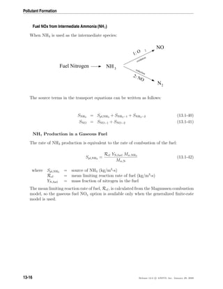
![13.1 NOx Formation
NH3 Production in a Liquid Fuel
The rate of NH3 production is equivalent to the rate of fuel release into the gas phase
through droplet evaporation:
Spl,NH3 =
Sfuel YN,fuel Mw,NH3
Mw,NV
(13.1-43)
where Spl,NH3 = source of NH3 (kg/m3
-s)
Sfuel = rate of fuel release from the liquid droplets to the gas (kg/s)
YN,fuel = mass fraction of nitrogen in the fuel
V = cell volume (m3
)
NH3 Consumption
The NH3 depletion rates from reactions (1) and (2) in the above mechanism are the same
for both gaseous and liquid fuels, and are given by De Soete [69] as
R1 = A1 XNH3 Xa
O2
e−E1/RT
(13.1-44)
R2 = A2 XNH3 XNO e−E2/RT
(13.1-45)
where R1, R2 = conversion rates of NH3 (s−1
)
T = instantaneous temperature (K)
X = mole fractions
A1 = 4.0 ×10⁶
s−1
A2 = 1.8 ×10⁸
s−1
E1 = 133947.2 J/gmol
E2 = 113017.95 J/gmol
The oxygen reaction order, a, is calculated from Equation 13.1-28.
Since mole fraction is related to mass fraction through molecular weights of the species
(Mw,i) and the mixture (Mw,m), Xi can be calculated using Equation 13.1-35.
Release 12.0 c ANSYS, Inc. January 29, 2009 13-17](https://image.slidesharecdn.com/flth-130501182911-phpapp02/85/Flth-377-320.jpg)
![13.1 NOx Formation
Coal Fuel NOx Scheme A
The first HCN mechanism assumes that all char N converts to HCN which is then con-
verted partially to NO [327]. The reaction pathway is described as follows:
HCN NO
Char N
Volatile N
2: NO
3: Char
N2
1: O 2 N2
With the first scheme, all char-bound nitrogen converts to HCN. Thus,
Schar,HCN =
ScYN,charMw,HCN
Mw,NV
(13.1-50)
Schar,NO = 0 (13.1-51)
where Sc = char burnout rate (kg/s)
YN,char = mass fraction of nitrogen in char
V = cell volume (m3
)
Coal Fuel NOx Scheme B
The second HCN mechanism assumes that all char N converts to NO directly [207]. The
reaction pathway is described as follows:
HCN NO
Char N
Volatile N
2: NO
3: Char
N2
1: O 2 N2
Release 12.0 c ANSYS, Inc. January 29, 2009 13-19](https://image.slidesharecdn.com/flth-130501182911-phpapp02/85/Flth-379-320.jpg)
![Pollutant Formation
According to Lockwood [207], the char nitrogen is released to the gas phase as NO directly,
mainly as a desorption product from oxidized char nitrogen atoms. If this approach is
followed, then
Schar,HCN = 0 (13.1-52)
Schar,NO =
ScYN,charMw,NO
Mw,NV
(13.1-53)
HCN Scheme Selection
The second HCN mechanism tends to produce more NOx emission than the first. In
general, however, it is difficult to say which one outperforms the other.
The source terms for the transport equations are
SHCN = Spvc,HCN + SHCN−1 + SHCN−2 (13.1-54)
SNO = Schar,NO + SNO−1 + SNO−2 + SNO−3 (13.1-55)
Source contributions SHCN−1, SHCN−2, SNO−1, and SNO−2 are described previously. There-
fore, only the heterogeneous reaction source, SNO−3, the char NOx source, Schar,NO, and
the HCN production source, Spvc,HCN, need to be considered.
NOx Reduction on Char Surface
The heterogeneous reaction of NO reduction on the char surface has been modeled ac-
cording to the following [190]:
R3 = A3e−E3/RT
pNO (13.1-56)
where R3 = rate of NO reduction (gmol/m2
BET-s)
pNO = mean NO partial pressure (atm)
E3 = 142737.485 J/gmol
A3 = 230 gmol/m2
BET-s-atm
T = mean temperature (K)
The partial pressure pNO is calculated using Dalton’s law:
pNO = pXNO
13-20 Release 12.0 c ANSYS, Inc. January 29, 2009](https://image.slidesharecdn.com/flth-130501182911-phpapp02/85/Flth-380-320.jpg)
![13.1 NOx Formation
The rate of NO consumption due to reaction 3 will then be
SNO−3 = csABETMw,NOR3
where ABET = BET surface area (m2
/kg)
cs = concentration of particles (kg/m3
)
SNO−3 = NO consumption (kg/m3
-s)
BET Surface Area
The heterogeneous reaction involving char is mainly an adsorption process whose rate is
directly proportional to the pore surface area. The pore surface area is also known as the
BET surface area due to the researchers who pioneered the adsorption theory (Brunauer,
Emmett and Teller [42]). For commercial adsorbents, the pore (BET) surface areas range
from 100,000 to 2 million square meters per kilogram, depending on the microscopic
structure. For coal, the BET area is typically 25,000 m2
/kg which is used as the default
in ANSYS FLUENT. The overall source of HCN (Spvc,HCN) is a combination of volatile
contribution (Svol,HCN) and char contribution (Schar,HCN):
Spvc,HCN = Svol,HCN + Schar,HCN
HCN from Volatiles
The source of HCN from the volatiles is related to the rate of volatile release:
Svol,HCN =
Svol YN,volMw,HCN
Mw,NV
where Svol = source of volatiles originating from
the coal particles into the gas phase (kg/s)
YN,vol = mass fraction of nitrogen in the volatiles
V = cell volume (m3
)
Calculation of sources related to char-bound nitrogen depends on the fuel NOx scheme
selection.
Release 12.0 c ANSYS, Inc. January 29, 2009 13-21](https://image.slidesharecdn.com/flth-130501182911-phpapp02/85/Flth-381-320.jpg)
![Pollutant Formation
Coal Fuel NOx Scheme C
The first NH3 mechanism assumes that all char N converts to NH3 which is then converted
partially to NO [327]. The reaction pathway is described as follows:
NH NO
Char N
Volatile N
2: NO
3: Char
N2
1: O 2 N2
3
In this scheme, all char-bound nitrogen converts to NH3. Thus,
Schar,NH3 =
ScYN,charMw,NH3
Mw,NV
(13.1-57)
Schar,NO = 0 (13.1-58)
where Sc = char burnout rate (kg/s)
YN,char = mass fraction of nitrogen in char
V = cell volume (m3
)
Coal Fuel NOx Scheme D
The second NH3 mechanism assumes that all char N converts to NO directly [207]. The
reaction pathway is described as follows:
NH NO
Char N
Volatile N
2: NO
3: Char
N2
1: O 2 N23
13-22 Release 12.0 c ANSYS, Inc. January 29, 2009](https://image.slidesharecdn.com/flth-130501182911-phpapp02/85/Flth-382-320.jpg)
![13.1 NOx Formation
According to Lockwood [207], the char nitrogen is released to the gas phase as NO directly,
mainly as a desorption product from oxidized char nitrogen atoms. If this approach is
followed, then
Schar,NH3 = 0 (13.1-59)
Schar,NO =
ScYN,charMw,NO
Mw,NV
(13.1-60)
NH3 Scheme Selection
The second NH3 mechanism tends to produce more NOx emission than the first. In
general, however, it is difficult to say which one outperforms the other.
The source terms for the transport equations are
SNH3 = Spvc,NH3 + SNH3−1 + SNH3−2 (13.1-61)
SNO = Schar,NO + SNO−1 + SNO−2 + SNO−3 (13.1-62)
Source contributions SNH3−1, SNH3−2, SNO−1, SNO−2, SNO−3, Schar,NO are described previ-
ously. Therefore, only the NH3 production source, Spvc,NH3 , needs to be considered.
The overall production source of NH3 is a combination of volatile contribution (Svol,NH3 ),
and char contribution (Schar,NH3 ):
Spvc,NH3 = Svol,NH3 + Schar,NH3 (13.1-63)
NH3 from Volatiles
The source of NH3 from the volatiles is related to the rate of volatile release:
Svol,NH3 =
Svol YN,volMw,NH3
Mw,NV
where Svol = source of volatiles originating from
the coal particles into the gas phase (kg/s)
YN,vol = mass fraction of nitrogen in the volatiles
V = cell volume (m3
)
Calculation of sources related to char-bound nitrogen depends on the fuel NOx scheme
selection.
Release 12.0 c ANSYS, Inc. January 29, 2009 13-23](https://image.slidesharecdn.com/flth-130501182911-phpapp02/85/Flth-383-320.jpg)
![Pollutant Formation
Fuel Nitrogen Partitioning for HCN and NH3 Intermediates
In certain cases, especially when the fuel is a solid, both HCN and NH3 can be generated
as intermediates at high enough temperatures [247]. In particular, low-ranking (lignite)
coal has been shown to produce 10 times more NH3 compared to the level of HCN,
whereas higher-ranking (bituminous) coal has been shown to produce only HCN [246].
Studies by Winter et al. [381] have shown that for bituminous coal, using an HCN/NH3
partition ratio of 9:1 gave better NOx predictions when compared to measurements than
specifying only a single intermediate species. Liu and Gibbs [206] work with woody-
biomass (pine wood chips), on the other hand, has suggested an HCN/NH3 ratio of 1:9
due to the younger age of the fuel.
In total, the above work suggests the importance of being able to specify that portions
of the fuel nitrogen will be converted to both HCN and NH3 intermediates at the same
time. In ANSYS FLUENT, fuel nitrogen partitioning can be used whenever HCN or NH3
are intermediates for NOx production, though it is mainly applicable to solid fuels such
as coal and biomass. The reaction pathways and source terms for HCN and NH3 were
discussed in previous sections.
13.1.6 NOx Formation from Intermediate N2O
Melte and Pratt [222] proposed the first intermediate mechanism for NOx formation from
molecular nitrogen (N2) via nitrous oxide (N2O). Nitrogen enters combustion systems
mainly as a component of the combustion and dilution air. Under favorable conditions,
which are elevated pressures and oxygen-rich conditions, this intermediate mechanism
can contribute as much as 90% of the NOx formed during combustion. This makes
it particularly important in equipment such as gas turbines and compression-ignition
engines. Because these devices are operated at increasingly low temperatures to prevent
NOx formation via the thermal NOx mechanism, the relative importance of the N2O-
intermediate mechanism is increasing. It has been observed that about 30% of the NOx
formed in these systems can be attributed to the N2O-intermediate mechanism.
The N2O-intermediate mechanism may also be of importance in systems operated in
flameless mode (e.g., diluted combustion, flameless combustion, flameless oxidation, and
FLOX systems). In a flameless mode, fuel and oxygen are highly diluted in inert gases so
that the combustion reactions and resulting heat release are carried out in the diffuse zone.
As a consequence, elevated peaks of temperature are avoided, which prevents thermal
NOx. Research suggests that the N2O-intermediate mechanism may contribute about
90% of the NOx formed in flameless mode, and that the remainder can be attributed
to the prompt NOx mechanism. The relevance of NOx formation from N2O has been
observed indirectly, and theoretically speculated for a number of combustion systems
and by a number of researchers [12, 61, 112, 338, 344].
13-24 Release 12.0 c ANSYS, Inc. January 29, 2009](https://image.slidesharecdn.com/flth-130501182911-phpapp02/85/Flth-384-320.jpg)
![13.1 NOx Formation
N2O-Intermediate NOx Mechanism
The simplest form of the mechanism [222] takes into account two reversible elementary
reactions:
N2 + O + M N2O + M (13.1-64)
N2O + O 2NO (13.1-65)
Here, M is a general third body. Because the first reaction involves third bodies, the
mechanism is favored at elevated pressures. Both reactions involve the oxygen radical
O, which makes the mechanism favored at oxygen-rich conditions. While not always
justified, it is often assumed that the radical O atoms originate solely from the dissociation
of molecular oxygen,
1
2
O2 O (13.1-66)
According to the kinetic rate laws, the rate of NOx formation via the N2O-intermediate
mechanism is
d[NO]
dt
= 2 kf,2[N2O][O] − kr,2[NO]2
gmol/m3
-s (13.1-67)
To solve Equation 13.1-67, you will need to have first calculated [O] and [N2O].
It is often assumed that N2O is at quasi-steady-state (i.e., d[N2O]/dt = 0), which implies
[N2O] =
kf,1[N2][O][M] + kr,2[NO]2
kr,1[M] + kf,2[O]
(13.1-68)
The system of Equations 13.1-67–13.1-68 can be solved for the rate of NOx formation
when the concentration of N2, O2, and M, the kinetic rate constants for Equations 13.1-64
and 13.1-65, and the equilibrium constant of Equation 13.1-66 are known. The appear-
ance of NO in Equation 13.1-65 entails that coupling of the N2O mechanism with the
thermal NOx mechanism (and other NOx mechanisms).
kf,1 = 4.44 × 1032
T−8.358
e−28234/T
kr,1 = 4.00 × 10⁸
e−28234/T
kf,2 = 2.90 × 10⁷
e−11651/T
kr,2 = 1.45 × 10⁻²⁹
T9.259
e−11651/T
In the above expressions, kf,1 and kf,2 are the forward rate constants of Equations 13.1-64
and 13.1-65, and kr,1 and kr,2 are the corresponding reverse rate constants. The units for
kf,2, kr,1, and kr,2 are m3
/gmol-s, while kf,1 has units of m6
/gmol2
-s.
Release 12.0 c ANSYS, Inc. January 29, 2009 13-25](https://image.slidesharecdn.com/flth-130501182911-phpapp02/85/Flth-385-320.jpg)
![Pollutant Formation
13.1.7 NOx Reduction by Reburning
The design of complex combustion systems for utility boilers, based on air- and fuel-
staging technologies, involves many parameters and their mutual interdependence. These
parameters include local stoichiometry, temperature and chemical concentration field,
residence time distribution, velocity field, and mixing pattern. A successful application
of the in-furnace reduction techniques requires control of these parameters in an optimum
manner so as to avoid impairing the boiler performance. In the mid 1990s, global models
describing the kinetics of NOx destruction in the reburn zone of a staged combustion
system became available. Two of these models are described below.
Instantaneous Approach
The instantaneous NOx reburning mechanism is a pathway whereby NO reacts with
hydrocarbons and is subsequently reduced. In general:
CHi + NO → HCN + products (13.1-69)
Three reburn reactions are modeled by ANSYS FLUENT for 1600 ≤ T ≤ 2100:
CH + NO
k1
→ HCN + O (13.1-70)
CH2 + NO
k2
→ HCN + OH (13.1-71)
CH3 + NO
k3
→ HCN + H2O (13.1-72)
i If the temperature is outside of this range, NO reburn will not be computed.
The rate constants for these reactions are taken from Bowman [32] and have units of
m3
/gmol-s:
k1 = 1 × 10⁸
; k2 = 1.4 × 10⁶
e−550/T
; k3 = 2 × 10⁵
The NO depletion rate due to reburn is expressed as
d[NO]
dt
= −k1[CH][NO] − k2[CH2][NO] − k3[CH3][NO] (13.1-73)
13-26 Release 12.0 c ANSYS, Inc. January 29, 2009](https://image.slidesharecdn.com/flth-130501182911-phpapp02/85/Flth-386-320.jpg)
![13.1 NOx Formation
and the source term for the reburning mechanism in the NO transport equation can be
calculated as
Sreburn,NO = −Mw,NO
d[NO]
dt
(13.1-74)
i To calculate the NO depletion rate due to reburning, ANSYS FLUENT will
obtain the concentrations of CH, CH2, and CH3 from the species mass
fraction results of the combustion calculation. When you use this method,
you must be sure to include the species CH, CH2, and CH3 in your problem
definition.
Partial Equilibrium Approach
The partial equilibrium approach is based on the model proposed by Kandamby et
al. [156] and [7]. The model adds a reduction path to De Soete’s global model [69]
that describes the NOx formation/destruction mechanism in a pulverized coal flame.
The additional reduction path accounts for the NOx destruction in the fuel-rich reburn
zone by CH radicals (see Figure 13.1.1).
N2
CHi
CHi
O2
HCN
NO Products
Fuel N
NO
(2)
(3)
(1)
(5)
(4)
Figure 13.1.1: De Soete’s Global NOx Mechanism with Additional Reduction
Path
This model can be used in conjunction with the eddy-dissipation combustion model and
does not require the specification of CH radical concentrations, since they are computed
based on the CH-radical partial equilibrium. The reburn fuel itself can be an equivalent of
CH4, CH3, CH2, or CH. How this equivalent fuel is determined is open for debate and an
approximate guide would be to consider the C/H ratio of the fuel itself. A multiplicative
constant of 4.0 × 10⁻⁴
has been developed for the partial equilibrium of CH radicals
to reduce the rates of HCN and NO in the reburn model. This value was obtained by
researchers, who developed the model, by way of predicting NOx values for a number of
test cases for which experimental data exists.
Release 12.0 c ANSYS, Inc. January 29, 2009 13-27](https://image.slidesharecdn.com/flth-130501182911-phpapp02/85/Flth-387-320.jpg)
![Pollutant Formation
NOx Reduction Mechanism
In the fuel-rich reburn zone, the HCN oxidation is suppressed and the amount of NO
formed in the primary combustion zone is decreased by the reduction reaction from HCN
to N2. However, the NO concentration may also decrease due to reactions with CH
radicals, which are available in significant amounts in the reburn zone. The following are
considered to be the most important reactions of NO reduction by CH radicals:
NO + CH2 −→ HCN + OH (13.1-75)
NO + CH −→ HCN + O (13.1-76)
NO + C −→ CN + O (13.1-77)
These reactions may be globally described by the addition of pathways (4) and (5) in
Figure 13.1.1, leading respectively to the formation of HCN and of minor intermediate
nitrogen radicals. Assuming that methane is the reburning gas, the global NO reduction
rates are then expressed as
R4 = (kaχ1 + kbχ2
1)[CH4][NO] (13.1-78)
R5 = kcχ3
1χ2[CH4][NO] (13.1-79)
where
χ1 =
[H]
[H2]
; χ2 =
[OH]
[H2O]
Therefore, the additional source terms of the HCN and NO transport equations due to
reburn reactions are given by
d[HCN]
dt
= 4 × 10⁻⁴
R4 (13.1-80)
d[NO]
dt
= −4 × 10⁻⁴
(R4 + R5) (13.1-81)
13-28 Release 12.0 c ANSYS, Inc. January 29, 2009](https://image.slidesharecdn.com/flth-130501182911-phpapp02/85/Flth-388-320.jpg)
![13.1 NOx Formation
Certain assumptions are required to evaluate the rate constants ka, kb, and kc and the
factors χ1 and χ2. For hydrocarbon diffusion flames, the following reaction set can be
reasonably considered to be in partial equilibrium:
CH4 + H CH3 + H2 (13.1-82)
CH3 + OH CH2 + H2O (13.1-83)
CH2 + H CH + H2 (13.1-84)
CH + H C + H2 (13.1-85)
Thus, the rate constants may be computed as
ka = k1
kf,4kf,5
kr,4kr,5
; kb = k2
kf,4kf,5kf,6
kr,4kr,5kr,6
; kc = k3
kf,4kf,5kf,6kf,7
kr,4kr,5kr,6kr,7
where k1, k2, and k3 are the rate constants for Equations 13.1-75–13.1-77. The forward
and reverse rate constants for Equations 13.1-82–13.1-85 are kf,4–kf,7 and kr,4–kr,7, re-
spectively. In addition, it is assumed that χ1 = 1, because the H-radical concentration
in the post-flame region of a hydrocarbon diffusion flame has been observed to be of the
same order as [H2]. Finally, the OH-radical concentration is estimated by considering the
reaction
OH + H2 H2O + H (13.1-86)
to be partially equilibrated, leading to the relationship
χ2 =
kr,8
kf,8
Values for the rate constants ka, kb, and kc for different equivalent fuel types are given
in Arrhenius form (ATb
e−E/RT
) in Table 13.1.1 [189]. All rate constants have units of
m3
/gmol-s, and all values of E have units of J/gmol.
Release 12.0 c ANSYS, Inc. January 29, 2009 13-29](https://image.slidesharecdn.com/flth-130501182911-phpapp02/85/Flth-389-320.jpg)
![Pollutant Formation
Table 13.1.1: Rate Constants for Different Reburn Fuels
Equivalent ka kb kc
Fuel Type A b E A b E A b E
CH4 5.30 × 10⁹
-1.54 27977 3.31 × 10¹³
-3.33 15090 3.06 × 10¹¹
-2.64 77077
CH3 0.37 × 10⁹
-1.54 27977 0.23 × 10¹³
-3.33 15090 0.21 × 10¹¹
-2.64 77077
CH2 0.23 × 10⁷
-1.54 27977 0.14 × 10¹¹
-3.33 15090 0.13 × 10⁹
-2.64 77077
CH 0.0 0.0 0.0 0.63 × 10⁸
-3.33 15090 0.58 × 10⁶
-2.64 77077
For Equation 13.1-86,
kf,8 = 1.02 × 10⁵
T1.60
e−13802/RT
; kr,8 = 4.52 × 10⁵
T1.60
e−80815/RT
13.1.8 NOx Reduction by SNCR
The selective noncatalytic reduction of NOx (SNCR), first described by Lyon [212], is a
method to reduce the emission of NOx from combustion by injecting a selective reductant
such as ammonia (NH3) or urea (CO(NH2)2) into the furnace, where it can react with NO
in the flue gas to form N2. However, the reductant can be oxidized as well to form NOx.
The selectivity for the reductive reactions decreases with increasing temperature [228]
while the rate of the initiation reaction simultaneously increases. This limits the SNCR
process to a narrow temperature interval, or window, where the lower temperature limit
for the interval is determined by the residence time.
Ammonia Injection
Several investigators have modeled the process using a large number of elementary reac-
tions. A simple empirical model has been proposed by Fenimore [92], which is based on
experimental measurements. However, the model was found to be unsuitable for practical
applications. Ostberg and Dam-Johansen [260] proposed a two-step scheme describing
the SNCR process as shown in Figure 13.1.2, which is a single initiation step followed
by two parallel reaction pathways: one leading to NO reduction, and the other to NO
formation.
13-30 Release 12.0 c ANSYS, Inc. January 29, 2009](https://image.slidesharecdn.com/flth-130501182911-phpapp02/85/Flth-390-320.jpg)
![13.1 NOx Formation
NH
3
OH
NH
2
OH
NO N2
NO
Figure 13.1.2: Simplified Reaction Mechanism for the SNCR Process
NO + NH3 +
1
4
O2 −→ N2 +
3
2
H2O (13.1-87)
NH3 +
5
4
O2 −→ NO +
3
2
H2O (13.1-88)
The reaction orders of NO and NH3 at 4% volume O2 and the empirical rate constants
kr and kox for Equations 13.1-87 and 13.1-88, respectively, have been estimated from
work done by Brouwer et al. [40]. The reaction order of NO was found to be 1 for
Equation 13.1-87 and the order of NH3 was found to be 1 for both reactions. As such,
the following reaction rates for NO and NH3, at 4% volume O2, were proposed:
RNO = −kr[NO][NH3] + kox[NH3][O2] (13.1-89)
RNH3 = −kr[NO][NH3] − kox[NH3][O2] (13.1-90)
The rate constants kr and kox have units of m3
/gmol-s, and are defined as
kr = 4.24 × 10²
T5.30
e−Er/RT
; kox = 3.50 × 10⁻¹
T7.65
e−Eox/RT
where Er = 349937.06 J/gmol and Eox = 524487.005 J/gmol.
Release 12.0 c ANSYS, Inc. January 29, 2009 13-31](https://image.slidesharecdn.com/flth-130501182911-phpapp02/85/Flth-391-320.jpg)
![Pollutant Formation
This model has been shown to give reasonable predictions of the SNCR process in pul-
verized coal and fluidized bed combustion applications. The model also captures the
influence of the most significant parameters for SNCR, which are the temperature of the
flue gas at the injection position, the residence time in the relevant temperature interval,
the NH3 to NO molar ratio, and the effect of combustible additives. This model overesti-
mates the NO reduction for temperatures above the optimum temperature by an amount
similar to that of the detailed kinetic model of Miller and Bowman [228].
i The SNCR process naturally occurs when NH3 is present in the flame as
a fuel N intermediate. For this reason, even if the SNCR model is not
activated and there is no reagent injection, the natural SNCR process may
still occur in the flame. The temperature range or “window” at which
SNCR may occur is 1073 K T 1373 K. To model your case without
using the natural SNCR process, please contact your support engineer for
information on how to deactivate it.
Urea Injection
Urea as a reagent for the SNCR process is similar to that of injecting ammonia and has
been used in the power station combustors to reduce NO emissions successfully. However,
both reagents, ammonia and urea, have major limitations as a NOx reducing agent. The
narrow temperature “window” of effectiveness and mixing limitations are difficult factors
to handle in a large combustor. The use of urea instead of ammonia as the reducing
agent is attractive because of the ease of storage and handling of the reagent.
The SNCR process using urea is a combination of Thermal DeNOx (SNCR with am-
monia) and RAPRENOx (SNCR using cyanuric acid that, under heating, sublimes and
decomposes into isocyanic acid) since urea most probably decomposes into ammonia and
isocyanic acid [228].
One problem of SNCR processes using urea is that slow decay of HNCO as well as
the reaction channels leading to N2O and CO can significantly increase the emission
of pollutants other than NO. Urea seems to involve a significant emission of carbon-
containing pollutants, such as CO and HNCO.
Also, some experimental observations [297] show that SNCR using urea is effective in a
narrow temperature window that is shifted toward higher temperatures when compared
to Thermal DeNOx processes at the same value of the ratio of nitrogen in the reducing
agent and in NO in the feed, β. The effect of increasing the β value is to increase the
efficiency of abatement, while the effect of increasing O2 concentration depends on the
temperature considered.
13-32 Release 12.0 c ANSYS, Inc. January 29, 2009](https://image.slidesharecdn.com/flth-130501182911-phpapp02/85/Flth-392-320.jpg)
![13.1 NOx Formation
The model described here is proposed by Brouwer et al. [40] and is a seven-step reduced
kinetic mechanism. Brouwer et al. [40] assumes that the breakdown of urea is instan-
taneous and 1 mole of urea is assumed to produce 1.1 moles of NH3 and 0.9 moles of
HNCO. The work of Rota et al. [297] proposed a finite rate two-step mechanism for the
breakdown of urea into ammonia and HNCO.
The seven-step reduced mechanism is given in Table 13.1.2 and the two-step urea break-
down mechanism is given in Table 13.1.3.
Table 13.1.2: Seven-Step Reduced Mechanism for SNCR with Urea
Reaction A b E
NH3 + NO → N2 + H2O + H 4.24E+02 5.30 349937.06
NH3 + O2 → NO + H2O + H 3.500E-01 7.65 524487.005
HNCO + M → H + NCO + M 2.400E+08 0.85 284637.8
NCO + NO → N2O + CO 1.000E+07 0.00 -1632.4815
NCO + OH → NO + CO + H 1.000E+07 0.00 0
N2O + OH → N2 + O2 + H 2.000E+06 0.00 41858.5
N2O + M → N2 + O + M 6.900E+17 -2.5 271075.646
Table 13.1.3: Two-Step Urea Breakdown Process
Reaction A b E
CO(NH2)2 → NH3 + HNCO 1.27E+04 0 65048.109
CO(NH2)2 + H2O → 2NH3 + CO2 6.13E+04 0 87819.133
where the units of A, in Tables 13.1.2 and 13.1.3, are m-gmol-sec and E units are J/gmol.
Transport Equations for Urea, HNCO, and NCO
When the SNCR model with urea injection is employed, in addition to the usual transport
equations, ANSYS FLUENT solves the following three additional mass transport equations
for urea, HNCO and NCO species.
∂
∂t
(ρYCO(NH2)2
) + · (ρvYCO(NH2)2
) = · (ρDYCO(NH2)2
) + SCO(NH2)2
(13.1-91)
∂
∂t
(ρYHNCO) + · (ρvYHNCO) = · (ρDYHNCO) + SHNCO (13.1-92)
Release 12.0 c ANSYS, Inc. January 29, 2009 13-33](https://image.slidesharecdn.com/flth-130501182911-phpapp02/85/Flth-393-320.jpg)
![Pollutant Formation
13.1.9 NOx Formation in Turbulent Flows
The kinetic mechanisms of NOx formation and destruction described in the preceding
sections have all been obtained from laboratory experiments using either a laminar pre-
mixed flame or shock-tube studies where molecular diffusion conditions are well defined.
In any practical combustion system, however, the flow is highly turbulent. The turbulent
mixing process results in temporal fluctuations in temperature and species concentration
that will influence the characteristics of the flame.
The relationships among NOx formation rate, temperature, and species concentration are
highly nonlinear. Hence, if time-averaged composition and temperature are employed
in any model to predict the mean NOx formation rate, significant errors will result.
Temperature and composition fluctuations must be taken into account by considering
the probability density functions which describe the time variation.
The Turbulence-Chemistry Interaction Model
In turbulent combustion calculations, ANSYS FLUENT solves the density-weighted time-
averaged Navier-Stokes equations for temperature, velocity, and species concentrations
or mean mixture fraction and variance. To calculate NO concentration, a time-averaged
NO formation rate must be computed at each point in the domain using the averaged
flow-field information.
Methods of modeling the mean turbulent reaction rate can be based on either moment
methods [380] or probability density function (PDF) techniques [148]. ANSYS FLUENT
uses the PDF approach.
i The PDF method described here applies to the NOx transport equations
only. The preceding combustion simulation can use either the general-
ized finite-rate chemistry model by Magnussen and Hjertager or the non-
premixed combustion model. For details on these models, refer to Chap-
ters 7 and 8.
The PDF Approach
The PDF method has proven very useful in the theoretical description of turbulent
flow [149]. In the ANSYS FLUENT NOx model, a single- or joint-variable PDF in terms
of a normalized temperature, species mass fraction, or the combination of both is used to
predict the NOx emission. If the non-premixed or partially premixed combustion model
is used to model combustion, then a one- or two-variable PDF in terms of mixture frac-
tion(s) is also available. The mean values of the independent variables needed for the
PDF construction are obtained from the solution of the transport equations.
13-36 Release 12.0 c ANSYS, Inc. January 29, 2009](https://image.slidesharecdn.com/flth-130501182911-phpapp02/85/Flth-396-320.jpg)
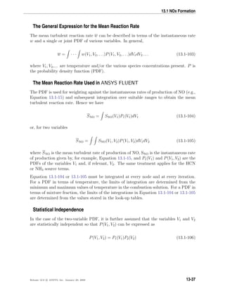
![Pollutant Formation
The Beta PDF Option
ANSYS FLUENT can assume P to be a two-moment beta function that is appropriate for
combustion calculations [123, 231]. The equation for the beta function is
P(V ) =
Γ(α + β)
Γ(α)Γ(β)
V α−1
(1 − V )β−1
=
V α−1
(1 − V )β−1
1
0
V α−1
(1 − V )β−1
dV
(13.1-107)
where Γ( ) is the Gamma function, α and β depend on m, the mean value of the quantity
in question, and its variance, σ2
:
α = m
m(1 − m)
σ2
− 1 (13.1-108)
β = (1 − m)
m(1 − m)
σ2
− 1 (13.1-109)
The beta function requires that the independent variable V assume values between 0 and
1. Thus, field variables such as temperature must be normalized. See Section 21.1.1: Set-
ting Turbulence Parameters in the separate User’s Guide for information on using the
beta PDF when using single-mixture fraction models and two-mixture fraction models.
The Gaussian PDF Option
ANSYS FLUENT can also assume P to exhibit a clipped Gaussian form with delta func-
tions at the tails.
The cumulative density function for a Gaussian PDF (GCDF) may be expressed in terms
of the error function as follows:
GCDF =
1
2
1 + erf (m − m) /
√
2σ2 (13.1-110)
where erf ( ) is the error function, m is the quantity in question, and m and σ2
are the
mean and variance values of m, respectively. The error function may be expressed in
terms of the incomplete gamma function (gammp( )):
for m 0 : erf(m) = −gammp(0.5, m2
)
for m ≥ 0 : erf(m) = gammp(0.5, m2
) (13.1-111)
13-38 Release 12.0 c ANSYS, Inc. January 29, 2009](https://image.slidesharecdn.com/flth-130501182911-phpapp02/85/Flth-398-320.jpg)
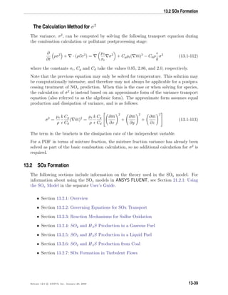
![Pollutant Formation
13.2.1 Overview
Sulfur exists in coal as organic sulfur, pyretic and sulfates [1], and exists in liquid fuels
mostly in organic form [235], with mass fractions ranging from 0.5% to 3%. All SOx
emissions are produced because of the oxidation of fuel-bound sulfur. During the com-
bustion process, fuel sulfur is oxidized to SO2 and SO3. A portion of the gaseous SOx
will condense on the particles, attaching an amount of water and thus forming sulfuric
acid, or may react further to form sulfates. While SOx emissions are the main cause of
acid rain, SO3 also contributes to particulate emissions, and is responsible for corrosion
of combustion equipment. Furthermore, there is a growing interest in the interaction
of sulfur species with the nitrogen oxide chemistry [235], as NO levels are affected by
the presence of sulfur species. The evidence to date indicates that thermal NO levels
(Section 13.1.3: Thermal NOx Formation) are reduced in the presence of SO2. However,
the effect of sulfur compounds on the fuel NOx formation is yet to be clarified.
Sulfur emissions are regulated from stationary sources and from automotive fuels. Sul-
fur pollutants can be captured during the combustion process, or with after treatment
methods, such as wet or dry scrubbing. Coal fired boilers are by far the biggest single
SOx emissions source, accounting for over 50% of total SO2 emissions [55].
For higher sulfur concentrations in the fuel, the SOx concentration field should be resolved
together with the main combustion calculation using any of the ANSYS FLUENT reaction
models. For cases where the sulfur fraction in fuel is low, the post-processing option can
be used, which solves transport equations for H2S, SO2, SO, SH, and SO3.
The Formation of SOx
The SOx model incorporates the following stages:
1. Sulfur release from the fuel
For liquid fuels, one can conveniently assume that sulfur is released as H2S [235].
However, the process is more complicated in the case of coal; here some of the
sulfur is decomposed into the gas phase during devolatilization as H2S, COS, SO2
and CS2, while part of the sulfur is retained in the char to be oxidized at a later
stage. The percentage of sulfur retained in char is rank dependent [1].
2. Sulfur reaction in the gas phase
In oxygen rich flames the predominant sulfur species are SO, SO2 and SO3. At lower
oxygen concentrations H2S, S2 and SH are also present in significant proportions,
while SO3 becomes negligible [235]. In PCGC-3 as well as in the works of Norman
et al. [251] the gas phase sulfur species are assumed to be in equilibrium.
3. Sulfur retention in sorbents
Sulfur pollutants can be absorbed by sorbent particles, injected either in situ, or in
the post flame region.
13-40 Release 12.0 c ANSYS, Inc. January 29, 2009](https://image.slidesharecdn.com/flth-130501182911-phpapp02/85/Flth-400-320.jpg)
![Pollutant Formation
13.2.3 Reaction Mechanisms for Sulfur Oxidation
A detailed reaction mechanism for sulfur oxidation has been proposed by Kramlich [172].
The mechanism consists of 20 reversible reactions and includes 12 species (S, S2, SH, SO,
SO2, H2S, H, H2, OH, H2O, O and O2). The mechanism has been reduced to 8 steps and
10 species (with S and S2 removed), and validated in Perfectly Stirred Reactor (PSR)
and Plug Flow Reactor (PFR) simulations. Table 13.2.1 lists the reduced mechanism
with the modified rate constants. For reduction calculations O and OH concentrations
have been calculated through partial equilibrium assumptions based on O2 and H2O
concentrations, respectively. N2 was used as the dilutant. Since each reaction of the
eight-step reduced mechanism is reversible, for each adjacent pair of reactions given in
Table 13.2.1, the second reaction is in fact the reverse reaction of the first.
The reduced mechanism given in Table 13.2.1 closely follows the SO2 concentration
levels but slightly overpredicts the H2S concentrations at temperatures below 1500 K.
Above 1500 K, both mechanisms are in close agreement for SO2 and H2S concentration
predictions. However, SO and SH are not well correlated by the reduced mechanism
when compared against the predictions using the original detailed mechanism.
A major concern in these mechanisms is the presence of H radical and the method in
which to calculate its concentration in the flow field. At present, the concentration of
H radical is assumed to be proportional to the O radical concentration, which can be
evaluated from one of the existing methods in ANSYS FLUENT; viz. Partial Equilib-
rium (Section 13.1.3: Method 2: Partial Equilibrium Approach) or Equilibrium (Sec-
tion 13.1.3: Method 1: Equilibrium Approach). The user is then given the option to
vary the proportionality constant. Although this assumption is open to debate, the lack
of simple relation to calculate the H radical concentration in a flame has prompted the
present choice.
Present implementation allows the user to either include or remove SO3 from the calcu-
lations. Also, depending on the form of fuel sulfur release (e.g., H2S or SO2) the species
H2S may or may not be present for the calculation. The user is also given the extended
option of partitioning the intermediate fuel sulfur species to H2S and SO2. However,
there is no literature to guide the user on how to select a correct partition fraction.
A is in m3
/gmol-s, E is J/gmol (assumed 1 cal = 4.18585 J), A units for the thirteenth
reaction is m6
/gmol2
-s, and A units for the fifteenth reaction is m6
/gmol2
-s.
In addition, the following two reactions were included in ANSYS FLUENT to complete
the SOx mechanism, with the rate constants taken from Hunter’s work [135].
SO2 + O + M ⇐⇒ SO3 + M (13.2-6)
M = argon, nitrogen, oxygen
kf1 = 3.63 x 10²
exp(+4185.85/RT) m6
/gmol2
/sec
13-42 Release 12.0 c ANSYS, Inc. January 29, 2009](https://image.slidesharecdn.com/flth-130501182911-phpapp02/85/Flth-402-320.jpg)
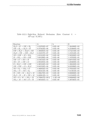
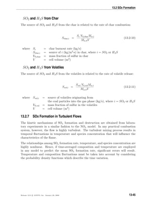
![Pollutant Formation
The Turbulence-Chemistry Interaction Model
In turbulent combustion calculations, ANSYS FLUENT solves the density-weighted time-
averaged Navier-Stokes equations for temperature, velocity, and species concentrations
or mean mixture fraction and variance. To calculate SO2 concentration, a time-averaged
SO2 formation rate must be computed at each point in the domain using the averaged
flow-field information.
The PDF Approach
The PDF method has proven very useful in the theoretical description of turbulent
flow [149]. In the ANSYS FLUENT SOx model, a single- or joint-variable PDF in terms
of a normalized temperature, species mass fraction, or the combination of both is used
to predict the SOx emission. If the non-premixed combustion model is used to model
combustion, then a one- or two-variable PDF in terms of mixture fraction(s) is also avail-
able. The mean values of the independent variables needed for the PDF construction are
obtained from the solution of the transport equations.
The Mean Reaction Rate
The mean turbulent reaction rate described in Section 13.1.9: The General Expression for
the Mean Reaction Rate for the NOx model also applies to the SOx model. The PDF is
used for weighting against the instantaneous rates of production of SO2 and subsequent
integration over suitable ranges to obtain the mean turbulent reaction rate as described
in Equations 13.1-104 and 13.1-105 for NOx.
The PDF Options
As is the case with the NOx model, P can be calculated as either a two-moment beta func-
tion or as a clipped Gaussian function, as appropriate for combustion calculations [123,
231]. Equations 13.1-107 – 13.1-111 apply to the SOx model as well, with the variance
σ2
computed by solving a transport equation during the combustion calculation stage,
using Equation 13.1-112 or Equation 13.1-113.
13-46 Release 12.0 c ANSYS, Inc. January 29, 2009](https://image.slidesharecdn.com/flth-130501182911-phpapp02/85/Flth-406-320.jpg)
![13.3 Soot Formation
13.3 Soot Formation
Information about the theory behind soot formation is presented in the following sec-
tions. For information about using soot formation models in ANSYS FLUENT, see Sec-
tion 21.3.1: Using the Soot Models in the separate User’s Guide.
• Section 13.3.1: Overview and Limitations
• Section 13.3.2: Soot Model Theory
13.3.1 Overview and Limitations
ANSYS FLUENT provides four models for the prediction of soot formation in combustion
systems. In addition, the predicted soot concentration can be coupled with radiation.
That is, you can include the effect of soot on radiation absorption when you use the
P-1, discrete ordinates, or discrete transfer radiation model with a variable absorption
coefficient.
Predicting Soot Formation
ANSYS FLUENT predicts soot concentrations in a combustion system using one of four
available models:
• the one-step Khan and Greeves model [162], in which ANSYS FLUENT predicts the
rate of soot formation based on a simple empirical rate
• the two-step Tesner model [216, 349], in which ANSYS FLUENT predicts the for-
mation of nuclei particles, with soot formation on the nuclei
• the Moss-Brookes model [39], in which ANSYS FLUENT predicts soot formation
for methane flames (and higher hydrocarbon species, if appropriately modified) by
solving transport equations for normalized radical nuclei concentration and the soot
mass fraction
• the Moss-Brookes-Hall model [120], which is an extension of the Moss-Brookes
model and is applicable for higher hydrocarbon fuels (e.g., kerosene)
The Khan and Greeves model is the default model used by ANSYS FLUENT when you
include soot formation.
Release 12.0 c ANSYS, Inc. January 29, 2009 13-47](https://image.slidesharecdn.com/flth-130501182911-phpapp02/85/Flth-407-320.jpg)
![Pollutant Formation
In the Khan and Greeves model and the Tesner model, combustion of the soot (and
particle nuclei) is assumed to be governed by the Magnussen combustion rate [216]. Note
that this limits the use of these soot formation models to turbulent flows. Both models
are empirically-based, approximate models of the soot formation process in combustion
systems. The detailed chemistry and physics of soot formation are quite complex and are
only approximated in these models. You should view the results of the Khan and Greeves
model and the Tesner model as qualitative indicators of your system performance unless
you can undertake experimental validation of the results.
The Moss-Brookes model has less impiricism and should theoretically provide superior
accuracy than the Khan and Greeves and Tesner models. The Hall extension provides
further options for modeling higher hydrocarbon fuels. Note that the Moss-Brookes-Hall
model is only available when the required species are present in the gas phase species
list.
Restrictions on Soot Modeling
The following restrictions apply to soot formation models:
• You must use the pressure-based solver. The soot models are not available with
either of the density-based solvers.
• The Khan and Greeves model and the Tesner model can model soot formation only
for turbulent flows (whereas the Moss-Brookes model and the Moss-Brookes-Hall
model can be used with both laminar and turbulent flows).
• The soot model cannot be used in conjunction with the premixed combustion model.
13.3.2 Soot Model Theory
The One-Step Soot Formation Model
In the one-step Khan and Greeves model [162], ANSYS FLUENT solves a single transport
equation for the soot mass fraction:
∂
∂t
(ρYsoot) + · (ρvYsoot) = ·
µt
σsoot
Ysoot + Rsoot (13.3-1)
where
Ysoot = soot mass fraction
σsoot = turbulent Prandtl number for soot transport
Rsoot = net rate of soot generation (kg/m3
-s)
Rsoot, the net rate of soot generation, is the balance of soot formation, Rsoot,form, and
soot combustion, Rsoot,comb:
13-48 Release 12.0 c ANSYS, Inc. January 29, 2009](https://image.slidesharecdn.com/flth-130501182911-phpapp02/85/Flth-408-320.jpg)
![13.3 Soot Formation
Rsoot = Rsoot,form − Rsoot,comb (13.3-2)
The rate of soot formation is given by a simple empirical rate expression:
Rsoot,form = Cspfuelφr
e−E/RT
(13.3-3)
where
Cs = soot formation constant (kg/N-m-s)
pfuel = fuel partial pressure (Pa)
φ = equivalence ratio
r = equivalence ratio exponent
E/R = activation temperature (K)
The rate of soot combustion is the minimum of two rate expressions [216]:
Rsoot,comb = min[R1, R2] (13.3-4)
The two rates are computed as
R1 = AρYsoot
k
(13.3-5)
and
R2 = Aρ
Yox
νsoot
Ysootνsoot
Ysootνsoot + Yfuelνfuel k
(13.3-6)
where
A = constant in the Magnussen model
Yox, Yfuel = mass fractions of oxidizer and fuel
νsoot, νfuel = mass stoichiometries for soot and fuel combustion
The default constants for the one-step model are valid for a wide range of hydrocarbon
fuels.
Release 12.0 c ANSYS, Inc. January 29, 2009 13-49](https://image.slidesharecdn.com/flth-130501182911-phpapp02/85/Flth-409-320.jpg)
![Pollutant Formation
The Two-Step Soot Formation Model
The two-step Tesner model [349] predicts the generation of radical nuclei and then com-
putes the formation of soot on these nuclei. ANSYS FLUENT thus solves transport
equations for two scalar quantities: the soot mass fraction (Equation 13.3-1) and the
normalized radical nuclei concentration:
∂
∂t
(ρb∗
nuc) + · (ρvb∗
nuc) = ·
µt
σnuc
b∗
nuc + R∗
nuc (13.3-7)
where
b∗
nuc = normalized radical nuclei concentration (particles ×10−15
/kg)
σnuc = turbulent Prandtl number for nuclei transport
R∗
nuc = normalized net rate of nuclei generation (particles ×10−15
/m3
-s)
In these transport equations, the rates of nuclei and soot generation are the net rates,
involving a balance between formation and combustion.
Soot Generation Rate
The two-step model computes the net rate of soot generation, Rsoot, in the same way as
the one-step model, as a balance of soot formation and soot combustion:
Rsoot = Rsoot,form − Rsoot,comb (13.3-8)
In the two-step model, however, the rate of soot formation, Rsoot,form, depends on the
concentration of radical nuclei, cnuc:
Rsoot,form = mp(α − βNsoot)cnuc (13.3-9)
where
mp = mean mass of soot particle (kg/particle)
Nsoot = concentration of soot particles (particles/m3
)
cnuc = radical nuclei concentration = ρbnuc (particles/m3
)
α = empirical constant (s−1
)
β = empirical constant (m3
/particle-s)
The rate of soot combustion, Rsoot,comb, is computed in the same way as for the one-step
model, using Equations 13.3-4–13.3-6.
The default constants for the two-step model are for combustion of acetylene (C2H2).
According to Ahmad et al. [2], these values should be modified for other fuels, since the
sooting characteristics of acetylene are known to be different from those of saturated
hydrocarbon fuels.
13-50 Release 12.0 c ANSYS, Inc. January 29, 2009](https://image.slidesharecdn.com/flth-130501182911-phpapp02/85/Flth-410-320.jpg)
![Pollutant Formation
The Moss-Brookes Model
The Moss-Brookes model solves transport equations for normalized radical nuclei con-
centration b∗
nuc and soot mass fraction Ysoot:
∂
∂t
(ρYsoot) + · (ρvYsoot) = ·
µt
σsoot
Ysoot +
dM
dt
(13.3-14)
∂
∂t
(ρb∗
nuc) + · (ρvb∗
nuc) = ·
µt
σnuc
b∗
nuc +
1
Nnorm
dN
dt
(13.3-15)
where
Ysoot = soot mass fraction
M = soot mass concentration (kg/m3
)
b∗
nuc = normalized radical nuclei concentration (particles ×10−15
/kg) = N
ρNnorm
N = soot particle number density (particles/m3
)
Nnorm = 1015
particles
The instantaneous production rate of soot particles, subject to nucleation from the gas
phase and coagulation in the free molecular regime, is given by
dN
dt
= CαNA
XprecP
RT
l
exp −
Tα
T
Nucleation
− Cβ
24RT
ρsootNA
1/2
d1/2
p N2
Coagulation
(13.3-16)
where Cα, Cβ and l are model constants. Here, NA (= 6.022045x1026
kmol−1
) is the
Avogadro number and Xprec is the mole fraction of soot precursor (for methane, the
precursor is assumed to be acetylene, whereas for kerosene it is a combination of acetylene
and benzene). The mass density of soot, ρsoot, is assumed to be 1800 kg/m3
and dp is
the mean diameter of a soot particle. The nucleation rate for soot particles is taken
to be proportional to the local acetylene concentration for methane. The activation
temperature Tα for the nucleation reaction is that proposed by Lindstedt [199].
13-52 Release 12.0 c ANSYS, Inc. January 29, 2009](https://image.slidesharecdn.com/flth-130501182911-phpapp02/85/Flth-412-320.jpg)
![13.3 Soot Formation
The source term for soot mass concentration is modeled by the expression
dM
dt
= MPCα
XprecP
RT
l
exp −
Tα
T
Nucleation
+ Cγ
XsgsP
RT
m
exp −
Tγ
T
(πN)1/3 6M
ρsoot
2/3
n
Surface Growth
− CoxidCωηcoll
XOHP
RT
√
T (πN)1/3 6M
ρsoot
2/3
Oxidation
(13.3-17)
where Cγ, Coxid, Cω, m, and n are additional model constants. The constant MP (= 144
kg/kgmol) is the mass of an incipient soot particle, here taken to consist of 12 carbon
atoms. Even though the model is not found to be sensitive to this assumption, a nonzero
initial mass is needed to begin the process of surface growth. Here, Xsgs is the mole
fraction of the participating surface growth species. For paraffinic fuels, soot particles
have been found to grow primarily by the addition of gaseous species at their surfaces,
particularly acetylene that has been found in abundance in the sooting regions of laminar
methane diffusion flames.
The model assumes that the hydroxyl radical is the dominant oxidizing agent in methane/air
diffusion flames and that the surface-specific oxidation rate of soot by the OH radical may
be formulated according to the model proposed by Fenimore and Jones [93]. Assuming a
collision efficiency (ηcoll) of 0.04, the oxidation rate may be written as (Equation 13.3-17.
The process of determination of the exponents l, m, and n are explained in detail by
Brookes and Moss [39]. The constants Cα and Cβ are determined through numerical
modeling of a laminar flame for which experimental data exists.
The set of constants proposed by Brookes and Moss for methane flames are given below:
Cα = 54 s−1
(model constant for soot inception rate)
Tα = 21000 K (activation temperature of soot inception)
Cβ = 1.0 (model constant for coagulation rate)
Cγ = 11700 kg.m.kmol−1
.s−1
(surface growth rate scaling factor)
Tγ = 12100 K (activation temperature of surface growth rate)
Cω = 105.8125 kg.m.kmol−1
.K−1/2
.s−1
(oxidation model constant)
ηcoll = 0.04 (collisional efficiency parameter)
Coxid = 0.015 (oxidation rate scaling parameter)
Note that the implementation of the Moss-Brookes model in ANSYS FLUENT uses the
values listed above, except for Coxid which is set to unity by default.
The closure for the mean soot source terms in the above equations was also described in
detail by Brookes and Moss [39]. The uncorrelated closure is the preferred option for a
tractable solution of the above transport equations.
Release 12.0 c ANSYS, Inc. January 29, 2009 13-53](https://image.slidesharecdn.com/flth-130501182911-phpapp02/85/Flth-413-320.jpg)
![Pollutant Formation
Moss et al. [239] have shown the above model applied to kerosene flames by modifying only
the soot precursor species (in the original model the precursor was acetylene, whereas
for kerosene flames the precursor was assumed to be a combination of both acetylene
and benzene) and by setting the value of oxidation scaling parameter Coxid to unity. A
good comparison against the experimental measurements for the lower pressure (7 bar)
conditions was observed. The predictions of soot formation within methane flames have
shown the Brooks and Moss [39] model to be superior compared with the standard Tesner
et al. [349] formulation.
The Coal-Derived Soot Extension (Beta Feature)
The present implementation provides an extension to the Moss-Brookes soot model that
accounts for coal-derived soot, based on the work of Brown [41]. This extension includes
an additional transport equation for the tar evolved during coal devolatilization. The
Moss-Brookes model assumes that the physical properties of tar is similar to those of
volatiles, such that the combined effect of volatile and tar on the gas phase flame sim-
ulation may be replaced by a single volatile stream (consisting of volatile and tar). In
reality, however, this may not be the case, and so the coal-derived soot extension allows
you to treat the tar contribution similar to that of volatiles.
The following set of paths was assumed for the coal-derived soot formation [214] (see
Figure 13.3.1).
Coal Char + Light Gases + Tar
Tar
Primary Soot
Light Gases
Soot Agglomerates
Devolatilization
Formation
Gasification
Agglomeration
Figure 13.3.1: Presumed Path for Coal-Derived Soot
13-54 Release 12.0 c ANSYS, Inc. February 9, 2009](https://image.slidesharecdn.com/flth-130501182911-phpapp02/85/Flth-414-320.jpg)
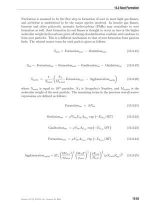
![Pollutant Formation
The soot oxidation term (Oxidationsoot) is similar to that shown in Equation 13.3-17
in the Moss-Brookes soot model theory (Fenimore-Jones or Lee oxidation model). Soot
density (ρsoot) is assumed to be 1950 kg/m3
and the collision constant Ca is set to 3.0.
Mw,C (= 12 kg/kgmol) is the molecular weight of carbon and kB (= 1.3806503e-23 J/K)
is the Boltzmann constant. An incipient soot particle is assumed to consist of 9e+04
carbon atoms, thus making Mw,soot = 108e+04 kg/kgmol. b∗
nuc is the normalized radical
nuclei concentration (i.e., the number of particles ×10−15
/kg). Since the coal-derived
soot particles are large, the turbulent Schmidt number used in the transport equations
for soot mass fraction and the normalized number density must be modified to account
for the particle size. A value of 700 for the turbulent Schmidt number is suggested for
soot mass fraction and nuclei transport.
The term SPtar is the tar release rate from coal (kg/m3
-s) and comes from the coal
particle source computations of the discrete phase model. It is assumed that the mass
fraction of tar in coal volatiles is in the range 0.3–0.5, and therefore the SPtar term is
related to the volatile source term via the tar mass fraction in volatiles. One of the main
assumptions of this implementation is that tar may be decoupled from the flow field
computations, since tar is a fraction of volatiles and volatile transport is fully coupled
with the flow field.
The values used for the pre-exponential constant A and the activation energy E in Equa-
tions 13.3-22–13.3-24 are listed in Table 13.3.1.
Table 13.3.1: Rate Constants for Coal-Derived Soot
Term A E (kJ/kgmol)
Oxidationtar 6.77e+05 (m3
/kg-s) 52,300
Gasificationtar 9.77e+10 (1/s) 286,900
Formationsoot 5.02e+08 (1/s) 198,900
The Moss-Brookes-Hall Model
Since the Moss-Brookes model was mainly developed and validated for methane flames,
a further extension for higher hydrocarbon fuels called the Moss-Brookes-Hall model was
also included in the present ANSYS FLUENT implementation. Here, the extended version
is a model reported by Wen et al. [374] based on model extensions proposed by Hall et
al. [120] and an oxidation model proposed by Lee et al. [184]. The work of Hall [120] is
based on a soot inception rate due to two-ringed and three-ringed aromatics, as opposed
to the Moss-Brookes assumption of a soot inception due to acetylene or benzene (for
higher hydrocarbons).
13-56 Release 12.0 c ANSYS, Inc. January 29, 2009](https://image.slidesharecdn.com/flth-130501182911-phpapp02/85/Flth-416-320.jpg)
![13.3 Soot Formation
Hall et al. [120] proposed a soot inception rate based on the formation rates of two-ringed
and three-ringed aromatics (C10H7 and C14H10), from acetylene (C2H2), benzene (C6H6),
and the phenyl radical (C6H5) based on the following mechanisms:
2 C2H2 + C6H5 C10H7 + H2 (13.3-26)
C2H2 + C6H6 + C6H5 C14H10 + H + H2 (13.3-27)
Based on their laminar methane flame data, the inception rate of soot particles was given
to be eight times the formation rate of species C10H7 and C14H10, as shown by
dN
dt inception
= 8Cα,1
NA
MP
ρ2 YC2H2
WC2H2
2
YC6H5 WH2
WC6H5 YH2
exp −
Tα,1
T
+8Cα,2
NA
MP
ρ2 YC2H2
WC2H2
YC6H6 YC6H5 WH2
WC6H6 WC6H5 YH2
exp −
Tα,2
T
(13.3-28)
where Cα,1 = 127x108.88
s−1
, Cα,2 = 178x109.50
s−1
, Tα,1 = 4378 K, and Tα,2 = 6390 K
as determined by Hall et al. [120]. In their model, the mass of an incipient soot particle
was assumed to be 1200 kg/kgmol (corresponding to 100 carbon atoms, as opposed to
12 carbon atoms used by Brookes and Moss [39]). The mass density of soot was assumed
to be 2000 kg/m3
, which is also slightly different from the value used by Brookes and
Moss. [39]
Both the coagulation term and the surface growth term were formulated similar to those
used by Brookes and Moss [39] with a slight modification to the constant Cγ so that the
value is 9000.6 kg.m.kmol−1
.s−1
(based on the model developed by Lindstedt [200]).
For the soot oxidation term, oxidation due to O2 (based on measurements and model
based on Lee et al. [184]) was added, in addition to the soot oxidation due to the hydroxyl
radical. By assuming that the kinetics of surface reactions is the limiting mechanism and
that the particles are small enough to neglect the diffusion effect on the soot oxidation,
they derived the specific rate of soot oxidation by molecular oxygen. Therefore the full
soot oxidation term, including that due to hydroxyl radical, is of the form
dM
dt oxidation
= −CoxidCω,1ηcoll
XOHP
RT
√
T (πN)1/3 6M
ρsoot
2/3
−CoxidCω,2
XO2 P
RT
exp −
Tω,2
T
√
T (πN)1/3 6M
ρsoot
2/3
(13.3-29)
Release 12.0 c ANSYS, Inc. January 29, 2009 13-57](https://image.slidesharecdn.com/flth-130501182911-phpapp02/85/Flth-417-320.jpg)
![Pollutant Formation
Here, the collision efficiency is assumed to be 0.13 (compared to 0.04 used by Brookes
and Moss) and the oxidation rate scaling parameter is assumed to be unity. The model
constants used are as follows:
where
Cω,1 = 105.81 kg.m.kmol−1
.K−1/2
.s−1
(same as that used by Brookes and
Moss)
Cω,2 = 8903.51 kg.m.kmol−1
.K−1/2
.s−1
Tω,2 = 19778 K
Soot Formation in Turbulent Flows
The kinetic mechanisms of soot formation and destruction for the Moss-Brookes model
and the Hall extension are obtained from laboratory experiments in a similar fashion
to the NOx model. In any practical combustion system, however, the flow is highly
turbulent. The turbulent mixing process results in temporal fluctuations in temperature
and species concentration that will influence the characteristics of the flame.
The relationships among soot formation rate, temperature, and species concentration are
highly nonlinear. Hence, if time-averaged composition and temperature are employed
in any model to predict the mean soot formation rate, significant errors will result.
Temperature and composition fluctuations must be taken into account by considering
the probability density functions which describe the time variation.
The Turbulence-Chemistry Interaction Model
In turbulent combustion calculations, ANSYS FLUENT solves the density-weighted time-
averaged Navier-Stokes equations for temperature, velocity, and species concentrations
or mean mixture fraction and variance. To calculate soot concentration for the Moss-
Brookes model and the Hall extension, a time-averaged soot formation rate must be
computed at each point in the domain using the averaged flow-field information.
The PDF Approach
The PDF method has proven very useful in the theoretical description of turbulent
flow [149]. In the ANSYS FLUENT Moss-Brookes model and the Hall extension, a single-
or joint-variable PDF in terms of a normalized temperature, species mass fraction, or the
combination of both is used to predict the soot formation. If the non-premixed combus-
tion model is used to model combustion, then a one- or two-variable PDF in terms of
mixture fraction(s) is also available. The mean values of the independent variables needed
for the PDF construction are obtained from the solution of the transport equations.
13-58 Release 12.0 c ANSYS, Inc. January 29, 2009](https://image.slidesharecdn.com/flth-130501182911-phpapp02/85/Flth-418-320.jpg)
![13.3 Soot Formation
The Mean Reaction Rate
The mean turbulent reaction rate described in Section 13.1.9: The General Expression
for the Mean Reaction Rate for the NOx model also applies to the Moss-Brookes model
and the Hall extension. The PDF is used for weighting against the instantaneous rates
of production of soot and subsequent integration over suitable ranges to obtain the mean
turbulent reaction rate as described in Equations 13.1-104 and 13.1-105 for NOx.
The PDF Options
As is the case with the NOx model, P can be calculated as either a two-moment beta func-
tion or as a clipped Gaussian function, as appropriate for combustion calculations [123,
231]. Equations 13.1-107 – 13.1-111 apply to the Moss-Brookes model and Hall exten-
sion as well, with the variance σ2
computed by solving a transport equation during the
combustion calculation stage, using Equation 13.1-112 or Equation 13.1-113.
The Effect of Soot on the Radiation Absorption Coefficient
A description of the modeling of soot-radiation interaction is provided in Section 5.3.8: The
Effect of Soot on the Absorption Coefficient.
Release 12.0 c ANSYS, Inc. January 29, 2009 13-59](https://image.slidesharecdn.com/flth-130501182911-phpapp02/85/Flth-419-320.jpg)

![Aerodynamically Generated Noise
14.1.1 Direct Method
In this method, both generation and propagation of sound waves are directly computed
by solving the appropriate fluid dynamics equations. Prediction of sound waves always
requires time-accurate solutions to the governing equations. Furthermore, in most prac-
tical applications of the direct method, one has to employ governing equations that are
capable of modeling viscous and turbulence effects, such as unsteady Navier-Stokes equa-
tions (i.e., DNS), RANS equations, and filtered equations used in DES and LES.
The direct method is thus computationally difficult and expensive inasmuch as it requires
highly accurate numerics, very fine computational meshes all the way to receivers, and
acoustically nonreflecting boundary conditions. The computational cost becomes pro-
hibitive when sound is to be predicted in the far field (e.g., hundreds of chord-lengths in
the case of an airfoil). The direct method becomes feasible when receivers are in the near
field (e.g., cabin noise). In many such situations involving near-field sound, sounds (or
pseudo-sounds for that matter) are predominantly due to local hydrodynamic pressure
which can be predicted with a reasonable cost and accuracy.
Since sound propagation is directly resolved in this method, one normally needs to solve
the compressible form of the governing equations (e.g., compressible RANS equations,
compressible form of filtered equations for LES). Only in situations where the flow is low
and subsonic, and the receivers in the near field consist primarily of local hydrodynamic
pressure fluctuations (i.e., pseudo sound), can incompressible flow formulations be used.
However, this incompressible treatment will not permit you to simulate resonance and
feedback phenomena.
14.1.2 Integral Method Based on Acoustic Analogy
For predictions of mid- to far-field noise, the methods based on Lighthill’s acoustic anal-
ogy [195] offer viable alternatives to the direct method. In this approach, the near-field
flow obtained from appropriate governing equations such as unsteady RANS equations,
DES, or LES are used to predict the sound with the aid of analytically derived integral
solutions to wave equations. The acoustic analogy essentially decouples the propagation
of sound from its generation, allowing one to separate the flow solution process from the
acoustics analysis.
ANSYS FLUENT offers a method based on the Ffowcs Williams and Hawkings (FW-H)
formulation [95]. The FW-H formulation adopts the most general form of Lighthill’s
acoustic analogy, and is capable of predicting sound generated by equivalent acoustic
sources such as monopoles, dipoles, and quadrupoles. ANSYS FLUENT adopts a time-
domain integral formulation wherein time histories of sound pressure, or acoustic signals,
at prescribed receiver locations are directly computed by evaluating a few surface inte-
grals.
14-2 Release 12.0 c ANSYS, Inc. January 29, 2009](https://image.slidesharecdn.com/flth-130501182911-phpapp02/85/Flth-422-320.jpg)
![14.2 Acoustics Model Theory
14.2.1 The Ffowcs Williams and Hawkings Model
The Ffowcs Williams and Hawkings (FW-H) equation is essentially an inhomogeneous
wave equation that can be derived by manipulating the continuity equation and the
Navier-Stokes equations. The FW-H [38, 95] equation can be written as:
1
a2
0
∂2
p
∂t2
− 2
p =
∂2
∂xi∂xj
{TijH(f)}
−
∂
∂xi
{[Pijnj + ρui (un − vn)] δ(f)}
+
∂
∂t
{[ρ0vn + ρ (un − vn)] δ(f)} (14.2-1)
where
ui = fluid velocity component in the xi direction
un = fluid velocity component normal to the surface f = 0
vi = surface velocity components in the xi direction
vn = surface velocity component normal to the surface
δ(f) = Dirac delta function
H(f) = Heaviside function
p is the sound pressure at the far field (p = p − p0). f = 0 denotes a mathematical
surface introduced to “embed” the exterior flow problem (f 0) in an unbounded space,
which facilitates the use of generalized function theory and the free-space Green function
to obtain the solution. The surface (f = 0) corresponds to the source (emission) surface,
and can be made coincident with a body (impermeable) surface or a permeable surface
off the body surface. ni is the unit normal vector pointing toward the exterior region
(f 0), a0 is the far-field sound speed, and Tij is the Lighthill stress tensor, defined as
Tij = ρuiuj + Pij − a2
0 (ρ − ρ0) δij (14.2-2)
Pij is the compressive stress tensor. For a Stokesian fluid, this is given by
Pij = pδij − µ
∂ui
∂xj
+
∂uj
∂xi
−
2
3
∂uk
∂xk
δij (14.2-3)
The free-stream quantities are denoted by the subscript 0.
Release 12.0 c ANSYS, Inc. January 29, 2009 14-5](https://image.slidesharecdn.com/flth-130501182911-phpapp02/85/Flth-425-320.jpg)
![14.2 Acoustics Model Theory
The various subscripted quantities appearing in Equations 14.2-5 and 14.2-6 are the
inner products of a vector and a unit vector implied by the subscript. For instance,
Lr = L · ˆr = Liri and Un = U · n = Uini, where r and n denote the unit vectors in
the radiation and wall-normal directions, respectively. The dot over a variable denotes
source-time differentiation of that variable.
Please note the following remarks regarding the applicability of this integral solution:
• The FW-H formulation in ANSYS FLUENT can handle rotating surfaces as well as
stationary surfaces.
• It is not required that the surface f = 0 coincide with body surfaces or walls. The
formulation permits source surfaces to be permeable, and therefore can be placed
in the interior of the flow.
• When a permeable source surface (either interior or nonconformal sliding interface)
is placed at a certain distance off the body surface, the integral solutions given by
Equations 14.2-5 and 14.2-6 include the contributions from the quadrupole sources
within the region enclosed by the source surface. When using a permeable source
surface, the mesh resolution needs to be fine enough to resolve the transient flow
structures inside the volume enclosed by the permeable surface.
14.2.2 Broadband Noise Source Models
Proudman’s Formula
Proudman [280], using Lighthill’s acoustic analogy, derived a formula for acoustic power
generated by isotropic turbulence without mean flow. More recently, Lilley [196] red-
erived the formula by accounting for the retarded time difference which was neglected in
Proudman’s original derivation. Both derivations yield acoustic power due to the unit
volume of isotropic turbulence (in W/m3
) as
PA = αρ0
u3
u5
a5
0
(14.2-10)
where u and are the turbulence velocity and length scales, respectively, and a0 is
the speed of sound. α in Equation 14.2-10 is a model constant. In terms of k and ε,
Equation 14.2-10 can be rewritten as
PA = αερ0εM5
t (14.2-11)
where
Mt =
√
2k
a0
(14.2-12)
Release 12.0 c ANSYS, Inc. January 29, 2009 14-7](https://image.slidesharecdn.com/flth-130501182911-phpapp02/85/Flth-427-320.jpg)
![Aerodynamically Generated Noise
The rescaled constant, α , is set to 0.1 in ANSYS FLUENT based on the calibration of
Sarkar and Hussaini [301] using direct numerical simulation of isotropic turbulence.
ANSYS FLUENT can also report the acoustic power in dB, which is computed from
LP = 10 log
PA
Pref
(14.2-13)
where Pref is the reference acoustic power (Pref = 10−12
W/m3
by default).
The Proudman’s formula gives an approximate measure of the local contribution to total
acoustic power per unit volume in a given turbulence field. Proper caution, however,
should be taken when interpreting the results in view of the assumptions made in the
derivation, such as high Reynolds number, small Mach number, isotropy of turbulence,
and zero mean motion.
The Jet Noise Source Model
This source model for axisymmetric jets is based on the works of Goldstein [113] who
modified the model originally proposed by Ribner [293] to better account for anisotropy
of turbulence in axisymmetric turbulent jets.
In Goldstein’s model, the total acoustic power emitted by the unit volume of a turbulent
jet is computed from
PA(y) =
2π
0
π
0
I(r, θ; y)r2
sin θdθ dψ
= 2πr2
π
0
I(r, θ; y) sin θ dθ (14.2-14)
where r and θ are the radial and angular coordinates of the receiver location, and I(r, θ; y)
is the directional acoustic intensity per unit volume of a jet defined by
I(r, θ; y) =
12 ρ0 ω4
f L1 L2
2 u2
t1
2
5 π a5
0 r2
Dself
C5
+
24 ρ0 ω4
f L1 L4
2 u2
t1
π a5
0 r2
∂U
∂r
2
Dshear
C5
(14.2-15)
C in Equation 14.2-15 is the modified convection factor defined by
C = 1 − Mc cos θ (14.2-16)
and
Dself = 1 + 2(
M
9
− N) cos2
θ sin2
θ
+
1
3
M2
7
+ M − 1.5N(3 − 3N +
1.5
∆2
−
∆2
2
) sin4
θ (14.2-17)
Dshear = cos2
θ cos2
θ +
1
2
1
∆2
− 2N sin2
θ (14.2-18)
14-8 Release 12.0 c ANSYS, Inc. January 29, 2009](https://image.slidesharecdn.com/flth-130501182911-phpapp02/85/Flth-428-320.jpg)
![14.2 Acoustics Model Theory
The remaining parameters are defined as
∆ =
L2
L1
(14.2-19)
M =
3
2
∆ −
1
∆
2
(14.2-20)
N = 1 −
u2
t2
u2
t1
(14.2-21)
L1 =
u2
t1
3/2
(14.2-22)
L2 =
u2
t2
3/2
(14.2-23)
ωf = 2π
k
(14.2-24)
where u2
t1 and u2
t2 are computed differently depending on the turbulence model chosen for
the computation. When the RSM is selected, they are computed from the corresponding
normal stresses. For all other two-equation turbulence models, they are obtained from
u2
t1 =
8
9
k (14.2-25)
u2
t2 =
4
9
k (14.2-26)
ANSYS FLUENT reports the acoustic power both in the dimensional units (W/m3
) and
in dB computed from
LP = 10 log
PA
Pref
(14.2-27)
where Pref is the reference acoustic power (Pref = 10−12
W/m3
by default).
The Boundary Layer Noise Source Model
Far-field sound generated by turbulent boundary layer flow over a solid body at low
Mach numbers is often of practical interest. The Curle’s integral [64] based on acoustic
analogy can be used to approximate the local contribution from the body surface to the
total acoustic power. To that end, one can start with the Curle’s integral
p (x, t) =
1
4πa0 S
(xi − yi) ni
r2
∂p
∂t
(y, τ) dS(y) (14.2-28)
Release 12.0 c ANSYS, Inc. January 29, 2009 14-9](https://image.slidesharecdn.com/flth-130501182911-phpapp02/85/Flth-429-320.jpg)

![14.2 Acoustics Model Theory
The right side of Equation 14.2-32 can be considered as effective source terms responsible
for sound generation. Among them, the first three terms involving turbulence are the
main contributors. The first two terms denoted by Lsh are often referred to as “shear-
noise” source terms, since they involve the mean shear. The third term denoted by Lse
is often called the “self-noise” source term, as it involves turbulent velocity components
only.
The turbulent velocity field needed to compute the LEE source terms is obtained using
the method of stochastic noise generation and radiation (SNGR) [23]. In this method,
the turbulent velocity field and its derivatives are computed from a sum of N Fourier
modes.
u (x, t) = 2
N
n=1
˜un cos kn · x + ψn σn (14.2-33)
where ˜un, ψn, σn are the amplitude, phase, and directional (unit) vector of the nth
Fourier
mode associated with the wave-number vector kn.
Note that the source terms in the LEE are vector quantities, having two or three com-
ponents depending on the dimension of the problem at hand.
Source Terms in Lilley’s Equation
Lilley’s equation is a third-order wave equation that can be derived by combining the
conservation of mass and momentum of compressible fluids. When the viscous terms are
omitted, it can be written in the following form:
D
Dt
D2
Π
Dt2
−
∂
∂xj
a2 ∂Π
∂xj
+ 2
∂uk
∂xj
∂
∂xk
a2 ∂Π
∂xj
= −2
∂uk
∂xi
∂uj
∂xk
∂ui
∂xj
(14.2-34)
where Π = (1/γ) ln p
po
.
Lilley’s equation can be linearized about the underlying steady flow as
ui(x, t) = Ui(x) + ui(x, t) (14.2-35)
where u (x, t) is the turbulent velocity component.
Substituting Equation 14.2-35 into the source term of Equation 14.2-34, we have
S ≡ −2
∂uk
∂xi
∂uj
∂xk
∂ui
∂xj
= −2
∂Uk
∂xi
∂Uj
∂xk
∂Ui
∂xj
−2
∂uk
∂xi
∂uj
∂xk
∂ui
∂xj
Self-Noise Terms
−6
∂Uk
∂xi
∂Uj
∂xk
∂ui
∂xj
− 6
∂uk
∂xi
∂uj
∂xk
∂Ui
∂xj
Shear-Noise Terms
(14.2-36)
Release 12.0 c ANSYS, Inc. January 29, 2009 14-11](https://image.slidesharecdn.com/flth-130501182911-phpapp02/85/Flth-431-320.jpg)

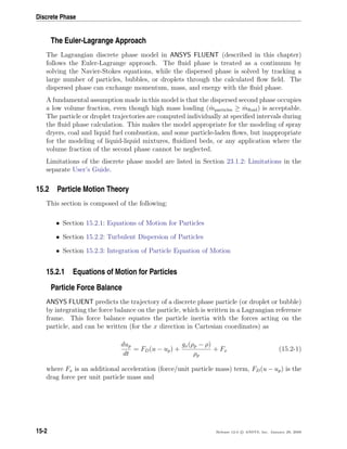
![Discrete Phase
where uy,p and uy are the particle and fluid velocities in the Cartesian y direction, and
1 −
ρ
ρp
Ω2
y − 2Ω ux,p −
ρ
ρp
ux (15.2-7)
where ux,p and ux are the particle and fluid velocities in the Cartesian x direction.
Thermophoretic Force
Small particles suspended in a gas that has a temperature gradient experience a force
in the direction opposite to that of the gradient. This phenomenon is known as ther-
mophoresis. ANSYS FLUENT can optionally include a thermophoretic effect on particles
in the additional acceleration (force/unit mass) term, Fx, in Equation 15.2-1:
Fx = −DT,p
1
mpT
∂T
∂x
(15.2-8)
where DT,p is the thermophoretic coefficient. You can define the coefficient to be constant,
polynomial, or a user-defined function, or you can use the form suggested by Talbot [345]:
Fx = −
6πdpµ2
Cs(K + CtKn)
ρ(1 + 3CmKn)(1 + 2K + 2CtKn)
1
mpT
∂T
∂x
(15.2-9)
where: Kn = Knudsen number = 2 λ/dp
λ = mean free path of the fluid
K = k/kp
k = fluid thermal conductivity based on translational
energy only = (15/4) µR
kp = particle thermal conductivity
CS = 1.17
Ct = 2.18
Cm = 1.14
mp = particle mass
T = local fluid temperature
µ = fluid viscosity
This expression assumes that the particle is a sphere and that the fluid is an ideal gas.
15-4 Release 12.0 c ANSYS, Inc. January 29, 2009](https://image.slidesharecdn.com/flth-130501182911-phpapp02/85/Flth-436-320.jpg)
![15.2 Particle Motion Theory
Brownian Force
For sub-micron particles, the effects of Brownian motion can be optionally included in the
additional force term. The components of the Brownian force are modeled as a Gaussian
white noise process with spectral intensity Sn,ij given by [191]
Sn,ij = S0δij (15.2-10)
where δij is the Kronecker delta function, and
S0 =
216νkBT
π2ρd5
p
ρp
ρ
2
Cc
(15.2-11)
T is the absolute temperature of the fluid, ν is the kinematic viscosity, and kB is the
Boltzmann constant. Amplitudes of the Brownian force components are of the form
Fbi
= ζi
πSo
∆t
(15.2-12)
where ζi are zero-mean, unit-variance-independent Gaussian random numbers. The am-
plitudes of the Brownian force components are evaluated at each time step. The energy
equation must be enabled in order for the Brownian force to take effect. Brownian force
is intended only for laminar simulations.
Saffman’s Lift Force
The Saffman’s lift force, or lift due to shear, can also be included in the additional force
term as an option. The lift force used is from Li and Ahmadi [191] and is a generalization
of the expression provided by Saffman [298]:
F =
2Kν1/2
ρdij
ρpdp(dlkdkl)1/4
(v − vp) (15.2-13)
where K = 2.594 and dij is the deformation tensor. This form of the lift force is in-
tended for small particle Reynolds numbers. Also, the particle Reynolds number based
on the particle-fluid velocity difference must be smaller than the square root of the par-
ticle Reynolds number based on the shear field. This option is recommended only for
submicron particles.
Release 12.0 c ANSYS, Inc. January 29, 2009 15-5](https://image.slidesharecdn.com/flth-130501182911-phpapp02/85/Flth-437-320.jpg)
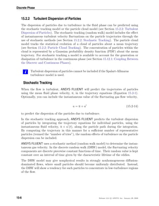
![15.2 Particle Motion Theory
The Integral Time
Prediction of particle dispersion makes use of the concept of the integral time scale, T,
which describes the time spent in turbulent motion along the particle path, ds:
T =
∞
0
up (t)up (t + s)
up
2
ds (15.2-15)
The integral time is proportional to the particle dispersion rate, as larger values indicate
more turbulent motion in the flow. It can be shown that the particle diffusivity is given
by ui uj T.
For small “tracer” particles that move with the fluid (zero drift velocity), the integral time
becomes the fluid Lagrangian integral time, TL. This time scale can be approximated as
TL = CL
k
(15.2-16)
where CL is to be determined as it is not well known. By matching the diffusivity of
tracer particles, ui uj TL, to the scalar diffusion rate predicted by the turbulence model,
νt/σ, one can obtain
TL ≈ 0.15
k
(15.2-17)
for the k- model and its variants, and
TL ≈ 0.30
k
(15.2-18)
when the Reynolds stress model (RSM) is used [67]. For the k-ω models, substitute
ω = /k into Equation 15.2-16. The LES model uses the equivalent LES time scales.
The Discrete Random Walk Model
In the discrete random walk (DRW) model, or “eddy lifetime” model, the interaction of
a particle with a succession of discrete stylized fluid phase turbulent eddies is simulated.
Each eddy is characterized by
• a Gaussian distributed random velocity fluctuation, u , v , and w
• a time scale, τe
Release 12.0 c ANSYS, Inc. January 29, 2009 15-7](https://image.slidesharecdn.com/flth-130501182911-phpapp02/85/Flth-439-320.jpg)
![Discrete Phase
The values of u , v , and w that prevail during the lifetime of the turbulent eddy are
sampled by assuming that they obey a Gaussian probability distribution, so that
u = ζ u 2 (15.2-19)
where ζ is a normally distributed random number, and the remainder of the right-hand
side is the local RMS value of the velocity fluctuations. Since the kinetic energy of
turbulence is known at each point in the flow, these values of the RMS fluctuating
components can be defined (assuming isotropy) as
u 2 = v 2 = w 2 = 2k/3 (15.2-20)
for the k- model, the k-ω model, and their variants. When the RSM is used, nonisotropy
of the stresses is included in the derivation of the velocity fluctuations:
u = ζ u 2 (15.2-21)
v = ζ v 2 (15.2-22)
w = ζ w 2 (15.2-23)
when viewed in a reference frame in which the second moment of the turbulence is diag-
onal [389]. For the LES model, the velocity fluctuations are equivalent in all directions.
See Section 4.11.4: Inlet Boundary Conditions for the LES Model for details.
The characteristic lifetime of the eddy is defined either as a constant:
τe = 2TL (15.2-24)
where TL is given by Equation 15.2-16 in general (Equation 15.2-17 by default), or as a
random variation about TL:
τe = −TL ln(r) (15.2-25)
where r is a uniform random number between 0 and 1 and TL is given by Equation 15.2-17.
The option of random calculation of τe yields a more realistic description of the correlation
function.
The particle eddy crossing time is defined as
tcross = −τ ln 1 −
Le
τ|u − up|
(15.2-26)
15-8 Release 12.0 c ANSYS, Inc. January 29, 2009](https://image.slidesharecdn.com/flth-130501182911-phpapp02/85/Flth-440-320.jpg)
![15.2 Particle Motion Theory
where τ is the particle relaxation time, Le is the eddy length scale, and |u − up| is the
magnitude of the relative velocity.
The particle is assumed to interact with the fluid phase eddy over the smaller of the
eddy lifetime and the eddy crossing time. When this time is reached, a new value of the
instantaneous velocity is obtained by applying a new value of ζ in Equation 15.2-19.
Using the DRW Model
The only inputs required for the DRW model are the value for the integral time-scale
constant, CL (see Equations 15.2-16 and 15.2-24) and the choice of the method used for
the prediction of the eddy lifetime. You can choose to use either a constant value or
a random value by selecting the appropriate option in the Set Injection Properties
dialog box for each injection, as described in Section 23.3.16: Stochastic Tracking in the
separate User’s Guide.
i Turbulent dispersion of particles cannot be included if the Spalart-Allmaras
turbulence model is used.
Particle Cloud Tracking
Particle dispersion due to turbulent fluctuations can also be modeled with the particle
cloud model [21, 22, 144, 204]. The turbulent dispersion of particles about a mean
trajectory is calculated using statistical methods. The concentration of particles about
the mean trajectory is represented by a Gaussian probability density function (PDF)
whose variance is based on the degree of particle dispersion due to turbulent fluctuations.
The mean trajectory is obtained by solving the ensemble-averaged equations of motion
for all particles represented by the cloud (see Section 15.2.2: Particle Cloud Tracking).
The cloud enters the domain either as a point source or with an initial diameter. The
cloud expands due to turbulent dispersion as it is transported through the domain until
it exits. As mentioned before, the distribution of particles in the cloud is defined by a
probability density function (PDF) based on the position in the cloud relative to the cloud
center. The value of the PDF represents the probability of finding particles represented
by that cloud with residence time t at location xi in the flow field. The average particle
number density can be obtained by weighting the total flow rate of particles represented
by that cloud, ˙m, as
n(xi) = ˙mP(xi, t) (15.2-27)
The PDFs for particle position are assumed to be multivariate Gaussian. These are
completely described by their mean, µi, and variance, σi
2
, and are of the form
Release 12.0 c ANSYS, Inc. January 29, 2009 15-9](https://image.slidesharecdn.com/flth-130501182911-phpapp02/85/Flth-441-320.jpg)
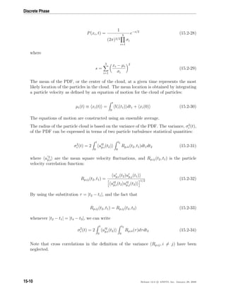
![15.2 Particle Motion Theory
The form of the particle velocity correlation function used determines the particle dis-
persion in the cloud model. ANSYS FLUENT uses a correlation function first proposed
by Wang [365], and used by Jain [144]. When the gravity vector is aligned with the
z-coordinate direction, Rij takes the form:
Rp,11 =
u 2
θ
e−(τ/τa)
StT B − 0.5mT γ
St2
T B2
+ 1
θ
+
u 2
θ
e−(τB/T)
−1 +
mT St2
T γB
θ
+ 0.5mT γ
τ
T
(15.2-35)
Rp,22 = Rp,11 (15.2-36)
Rp,33 =
u 2
StT B
θ
e−(τ/τa)
−
u 2
θ
e−(τB/T)
(15.2-37)
where B = 1 + m2
T γ2 and τa is the aerodynamic response time of the particle:
τa =
ρpd2
p
18µ
(15.2-38)
and
T =
mT TmE
m
(15.2-39)
TfE =
C3/4
µ k3/2
(2
3
k)1/2
(15.2-40)
γ =
τag
u
(15.2-41)
St =
τa
TmE
(15.2-42)
StT =
τa
T
(15.2-43)
θ = St2
T (1 + m2
T γ2
) − 1 (15.2-44)
m =
¯u
u
(15.2-45)
TmE = TfE
¯u
u
(15.2-46)
mT = m 1 −
G(m)
(1 + St)0.4(1+0.01St)
(15.2-47)
G(m) =
2
√
π
∞
0
e−y2
dy
1 + m2
π
(
√
π erf(y)y − 1 + e−y2
)
5/2
(15.2-48)
Release 12.0 c ANSYS, Inc. January 29, 2009 15-11](https://image.slidesharecdn.com/flth-130501182911-phpapp02/85/Flth-443-320.jpg)
![Discrete Phase
For the implicit and the trapezoidal schemes the new particle location is always computed
by a trapezoidal discretization of Equation 15.2-50.
xn+1
p = xn
p +
1
2
∆t un
p + un+1
p (15.2-60)
Equations 15.2-51 and 15.2-50 can also be computed using a Runge-Kutta scheme which
was published by Cash and Karp [48]. The ordinary differential equations can be con-
sidered as vectors, where the left hand side is the derivative y and the right hand side is
an arbitrary function f(t, y).
y = f(t, y) (15.2-61)
We get
yn+1
= yn
+ c1k1 + c2k2 + c3k3 + c4k4 + c5k5 + c6k6 (15.2-62)
with
k1 = ∆tf(t, yn
)
k2 = ∆tf(t + a2∆t, yn
+ b21k1)
k3 = ∆tf(t + a3∆t, yn
+ b31k1 + b32k2)
k4 = ∆tf(t + a4∆t, yn
+ b41k1 + b42k2 + b43k3)
k5 = ∆tf(t + a5∆t, yn
+ b51k1 + b52k2 + b53k3 + b54k4)
k6 = ∆tf(t + a6∆t, yn
+ b61k1 + b62k2 + b63k3 + b64k4 + b65k5)
The coefficients a2 . . . a6, b21 . . . b65, and c1 . . . c6 are taken from Cash and Karp [48]
This scheme provides an embedded error control, which is switched off, when no Accuracy
Control is enabled.
For rotating reference frames, the integration is carried out in the rotating frame with
the extra terms described in Equation 15.2-6 and Equation 15.2-7, thus accounting for
system rotation. Using the mechanisms available for accuracy control, the trajectory
integration will be done accurately in time.
The analytic scheme is very efficient. It can become inaccurate for large steps and in situ-
ations where the particles are not in hydrodynamic equilibrium with the continuous flow.
The numerical schemes implicit and trapezoidal, in combination with Automated Tracking
Scheme Selection, consider most of the changes in the forces acting on the particles and
are chosen as default schemes. The runge-kutta scheme is recommended of nondrag force
changes along a particle integration step.
15-14 Release 12.0 c ANSYS, Inc. January 29, 2009](https://image.slidesharecdn.com/flth-130501182911-phpapp02/85/Flth-446-320.jpg)
![15.3 Laws for Drag Coefficients
The integration step size of the higher-order schemes, trapezoidal and runge-kutta, is
limited to a stable range. Therefore it is recommended to use them in combination with
Automated Tracking Scheme Selection.
For the massless particle type, the particle velocity is equal to the velocity of the contin-
uous phase, hence the solution of only the trajectory Equation 15.2-50 is required where
the particle velocity up = u. The new particle location along the trajectory is always
computed by Equations 15.2-58 and 15.2-60, with up = u.
15.3 Laws for Drag Coefficients
Several laws for drag coefficients, CD, are available for the Euler-Lagrange Model.
Instructions for selecting the drag law are provided in Section 23.2.4: Drag Laws in the
separate User’s Guide.
15.3.1 Spherical Drag Law
The drag coefficient, CD, for smooth particles can be taken from
CD = a1 +
a2
Re
+
a3
Re2 (15.3-1)
where a1, a2, and a3 are constants that apply over several ranges of Re given by Morsi
and Alexander [238].
15.3.2 Non-spherical Drag Law
For non-spherical particles Haider and Levenspiel [119] developed the correlation
CD =
24
Resph
1 + b1Resph
b2
+
b3Resph
b4 + Resph
(15.3-2)
where
b1 = exp(2.3288 − 6.4581φ + 2.4486φ2
)
b2 = 0.0964 + 0.5565φ
b3 = exp(4.905 − 13.8944φ + 18.4222φ2
− 10.2599φ3
)
b4 = exp(1.4681 + 12.2584φ − 20.7322φ2
+ 15.8855φ3
) (15.3-3)
The shape factor, φ, is defined as
φ =
s
S
(15.3-4)
Release 12.0 c ANSYS, Inc. January 29, 2009 15-15](https://image.slidesharecdn.com/flth-130501182911-phpapp02/85/Flth-447-320.jpg)
![Discrete Phase
where s is the surface area of a sphere having the same volume as the particle, and S
is the actual surface area of the particle. The Reynolds number Resph is computed with
the diameter of a sphere having the same volume.
i The shape factor cannot exceed a value of 1.
15.3.3 Stokes-Cunningham Drag Law
For sub-micron particles, a form of Stokes’ drag law is available [261]. In this case, FD
is defined as
FD =
18µ
dp
2
ρpCc
(15.3-5)
The factor Cc is the Cunningham correction to Stokes’ drag law, which you can compute
from
Cc = 1 +
2λ
dp
(1.257 + 0.4e−(1.1dp/2λ)
) (15.3-6)
where λ is the molecular mean free path.
15.3.4 High-Mach-Number Drag Law
A high-Mach-number drag law is also available. This drag law is similar to the spherical
law (Equation 15.3-1) with corrections [57] to account for a particle Mach number greater
than 0.4 at a particle Reynolds number greater than 20.
15.3.5 Dynamic Drag Model Theory
Accurate determination of droplet drag coefficients is crucial for accurate spray mod-
eling. ANSYS FLUENT provides a method that determines the droplet drag coefficient
dynamically, accounting for variations in the droplet shape.
The dynamic drag model is applicable in almost any circumstance. It is compatible with
both the TAB and wave models for droplet breakup. When the collision model is turned
on, collisions reset the distortion and distortion velocities of the colliding droplets.
Many droplet drag models assume the droplet remains spherical throughout the domain.
With this assumption, the drag of a spherical object is determined by the following [205]:
Cd,sphere =
0.424 Re 1000
24
Re
1 + 1
6
Re2/3
Re ≤ 1000
(15.3-7)
15-16 Release 12.0 c ANSYS, Inc. January 29, 2009](https://image.slidesharecdn.com/flth-130501182911-phpapp02/85/Flth-448-320.jpg)
![15.3 Laws for Drag Coefficients
However, as an initially spherical droplet moves through a gas, its shape is distorted
significantly when the Weber number is large. In the extreme case, the droplet shape
will approach that of a disk. The drag of a disk, however, is significantly higher than that
of a sphere. Since the droplet drag coefficient is highly dependent upon the droplet shape,
a drag model that assumes the droplet is spherical is unsatisfactory. The dynamic drag
model accounts for the effects of droplet distortion, linearly varying the drag between
that of a sphere (Equation 15.3-7) and a value of 1.54 corresponding to a disk [205]. The
drag coefficient is given by
Cd = Cd,sphere(1 + 2.632y) (15.3-8)
where y is the droplet distortion, as determined by the solution of
d2
y
dt2
=
CF
Cb
ρg
ρl
u2
r2
−
Ckσ
ρlr3
y −
Cdµl
ρlr2
dy
dt
(15.3-9)
In the limit of no distortion (y = 0), the drag coefficient of a sphere will be obtained,
while at maximum distortion (y = 1) the drag coefficient corresponding to a disk will be
obtained.
Note that Equation 15.3-9 is obtained from the TAB model for spray breakup, described
in Section 15.10.1: Taylor Analogy Breakup (TAB) Model, but the dynamic drag model
can be used with either of the breakup models.
15.3.6 Dense Discrete Phase Model Drag Laws
The drag laws that are suitable for dense gas-solid flow are the Wen and Yu, the Gi-
daspow, and the Syamlal-O’Brien drag model. A detailed theoretical background to the
correlations, along with a recommendation of when to use each model, can be found in
Section 16.5.4: Fluid-Solid Exchange Coefficient (see also Section 24.5.2: Specifying the
Drag Function in the separate User’s Guide). All three correlations incorporate group
effects and therefore are dependent on the particle phase volume fraction. Thus, the
new drag models are only available when the DPM volume fraction is computed, i.e. in
conjunction with the Dense Discrete Phase Model.
Release 12.0 c ANSYS, Inc. January 29, 2009 15-17](https://image.slidesharecdn.com/flth-130501182911-phpapp02/85/Flth-449-320.jpg)

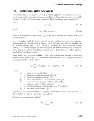
![Discrete Phase
where I is the radiation intensity and Ω is the solid angle.
Radiation heat transfer to the particle is included only if you have enabled the P-1 or
discrete ordinates radiation model and you have activated radiation heat transfer to
particles using the Particle Radiation Interaction option in the Discrete Phase Model
dialog box.
Equation 15.4-3 is integrated in time using an approximate, linearized form that assumes
that the particle temperature changes slowly from one time value to the next:
mpcp
dTp
dt
= Ap − h + pσT3
p Tp + hT∞ + pσθ4
R (15.4-5)
As the particle trajectory is computed, ANSYS FLUENT integrates Equation 15.4-5 to
obtain the particle temperature at the next time value, yielding
Tp(t + ∆t) = αp + [Tp(t) − αp]e−βp∆t
(15.4-6)
where ∆t is the integration time step and
αp =
hT∞ + pσθ4
R
h + pσT3
p (t)
(15.4-7)
and
βp =
Ap(h + pσT3
p (t))
mpcp
(15.4-8)
ANSYS FLUENT can also solve Equation 15.4-5 in conjunction with the equivalent mass
transfer equation using a stiff coupled solver. See Section 23.2.8: Including Coupled
Heat-Mass Solution Effects on the Particles in the separate User’s Guide for details.
The heat transfer coefficient, h, is evaluated using the correlation of Ranz and Mar-
shall [284, 285]:
Nu =
hdp
k∞
= 2.0 + 0.6Re
1/2
d Pr1/3
(15.4-9)
where
dp = particle diameter (m)
k∞ = thermal conductivity of the continuous phase (W/m-K)
Red = Reynolds number based on the particle diameter and
the relative velocity (Equation 15.2-3)
Pr = Prandtl number of the continuous phase (cpµ/k∞)
15-20 Release 12.0 c ANSYS, Inc. January 29, 2009](https://image.slidesharecdn.com/flth-130501182911-phpapp02/85/Flth-452-320.jpg)
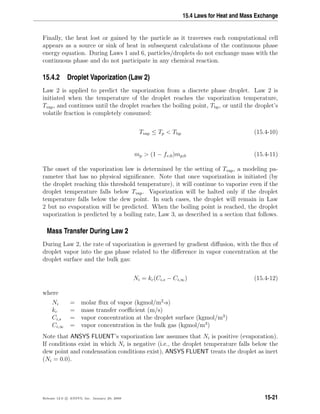
![Discrete Phase
The concentration of vapor at the droplet surface is evaluated by assuming that the
partial pressure of vapor at the interface is equal to the saturated vapor pressure, psat,
at the particle droplet temperature, Tp:
Ci,s =
psat(Tp)
RTp
(15.4-13)
where R is the universal gas constant.
The concentration of vapor in the bulk gas is known from solution of the transport
equation for species i for nonpremixed or partially premixed combustion calculations:
Ci,∞ = Xi
p
RT∞
(15.4-14)
where Xi is the local bulk mole fraction of species i, p is the local absolute pressure,
and T∞ is the local bulk temperature in the gas. The mass transfer coefficient in Equa-
tion 15.4-12 is calculated from the Sherwood number correlation [284, 285]:
ShAB =
kcdp
Di,m
= 2.0 + 0.6Re
1/2
d Sc1/3
(15.4-15)
where Di,m = diffusion coefficient of vapor in the bulk (m2
/s)
Sc = the Schmidt number, µ
ρDi,m
dp = particle (droplet) diameter (m)
The vapor flux given by Equation 15.4-12 becomes a source of species i in the gas phase
species transport equation, (see Section 23.5: Setting Material Properties for the Discrete
Phase in the separate User’s Guide) or in the mixture fraction equation for nonpremixed
combustion calculations.
The mass of the droplet is reduced according to
mp(t + ∆t) = mp(t) − NiApMw,i∆t (15.4-16)
where Mw,i = molecular weight of species i (kg/kgmol)
mp = mass of the droplet (kg)
Ap = surface area of the droplet (m2
)
ANSYS FLUENT can also solve Equation 15.4-16 in conjunction with the equivalent heat
transfer equation using a stiff coupled solver. See Section 23.2.8: Including Coupled
Heat-Mass Solution Effects on the Particles in the separate User’s Guide for details.
15-22 Release 12.0 c ANSYS, Inc. January 29, 2009](https://image.slidesharecdn.com/flth-130501182911-phpapp02/85/Flth-454-320.jpg)
![15.4 Laws for Heat and Mass Exchange
Defining the Vapor Pressure and Diffusion Coefficient
You must define the vapor pressure as a polynomial or piecewise linear function of tem-
perature (psat(T)) during the problem definition. Note that the vapor pressure definition
is critical, as psat is used to obtain the driving force for the evaporation process (Equa-
tions 15.4-12 and 15.4-13). You should provide accurate vapor pressure values for tem-
peratures over the entire range of possible droplet temperatures in your problem. Vapor
pressure data can be obtained from a physics or engineering handbook (e.g., [266]).
You must also input the diffusion coefficient, Di,m, during the setup of the discrete phase
material properties. Note that the diffusion coefficient inputs that you supply for the
continuous phase are not used in the discrete phase model.
Heat Transfer to the Droplet
Finally, the droplet temperature is updated according to a heat balance that relates the
sensible heat change in the droplet to the convective and latent heat transfer between
the droplet and the continuous phase:
mpcp
dTp
dt
= hAp(T∞ − Tp) +
dmp
dt
hfg + Ap pσ(θR
4
− Tp
4
) (15.4-17)
where cp = droplet heat capacity (J/kg-K)
Tp = droplet temperature (K)
h = convective heat transfer coefficient (W/m2
-K)
T∞ = temperature of continuous phase (K)
dmp
dt
= rate of evaporation (kg/s)
hfg = latent heat (J/kg)
p = particle emissivity (dimensionless)
σ = Stefan-Boltzmann constant (5.67 x 10⁻⁸
W/m2
-K4
)
θR = radiation temperature, ( I
4σ
)1/4
, where I is the radiation intensity
Radiation heat transfer to the particle is included only if you have enabled the P-1 or
discrete ordinates radiation model and you have activated radiation heat transfer to
particles using the Particle Radiation Interaction option in the Discrete Phase Model
dialog box.
The heat transferred to or from the gas phase becomes a source/sink of energy during
subsequent calculations of the continuous phase energy equation.
Release 12.0 c ANSYS, Inc. January 29, 2009 15-23](https://image.slidesharecdn.com/flth-130501182911-phpapp02/85/Flth-455-320.jpg)
![Discrete Phase
15.4.3 Droplet Boiling (Law 3)
Law 3 is applied to predict the convective boiling of a discrete phase droplet when the
temperature of the droplet has reached the boiling temperature, Tbp, and while the mass
of the droplet exceeds the nonvolatile fraction, (1 − fv,0):
Tp ≥ Tbp (15.4-18)
and
mp (1 − fv,0)mp,0 (15.4-19)
When the droplet temperature reaches the boiling point, a boiling rate equation is ap-
plied [173]:
d(dp)
dt
=
4k∞
ρpcp,∞dp
(1 + 0.23 Red) ln 1 +
cp,∞(T∞ − Tp)
hfg
(15.4-20)
where cp,∞ = heat capacity of the gas (J/kg-K)
ρp = droplet density (kg/m3
)
k∞ = thermal conductivity of the gas (W/m-K)
Equation 15.4-20 was derived assuming steady flow at constant pressure. Note that the
model requires T∞ Tbp in order for boiling to occur and that the droplet remains at
fixed temperature (Tbp) throughout the boiling law.
When radiation heat transfer is active, ANSYS FLUENT uses a slight modification of
Equation 15.4-20, derived by starting from Equation 15.4-17 and assuming that the
droplet temperature is constant. This yields
−
dmp
dt
hfg = hAp(T∞ − Tp) + Ap pσ(θR
4
− Tp
4
) (15.4-21)
or
−
d(dp)
dt
=
2
ρphfg
k∞Nu
dp
(T∞ − Tp) + pσ(θ4
R − T4
p ) (15.4-22)
Using Equation 15.4-9 for the Nusselt number correlation and replacing the Prandtl
number term with an empirical constant, Equation 15.4-22 becomes
−
d(dp)
dt
=
2
ρphfg
2k∞[1 + 0.23
√
Red]
dp
(T∞ − Tp) + pσ(θ4
R − T4
p ) (15.4-23)
15-24 Release 12.0 c ANSYS, Inc. January 29, 2009](https://image.slidesharecdn.com/flth-130501182911-phpapp02/85/Flth-456-320.jpg)
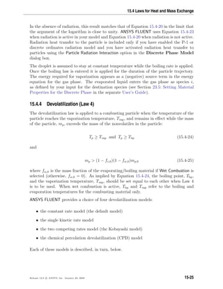
![Discrete Phase
Choosing the Devolatilization Model
You will choose the devolatilization model when you are setting physical properties for the
combusting-particle material in the Create/Edit Materials dialog box, as described in
Section 23.5.2: Description of the Properties in the separate User’s Guide. By default,
the constant rate model (Equation 15.4-26) will be used.
The Constant Rate Devolatilization Model
The constant rate devolatilization law dictates that volatiles are released at a constant
rate [20]:
−
1
fv,0(1 − fw,0)mp,0
dmp
dt
= A0 (15.4-26)
where mp = particle mass (kg)
fv,0 = fraction of volatiles initially present in the particle
mp,0 = initial particle mass (kg)
A0 = rate constant (s−1
)
The rate constant A0 is defined as part of your modeling inputs, with a default value of 12
s−1
derived from the work of Pillai [271] on coal combustion. Proper use of the constant
devolatilization rate requires that the vaporization temperature, which controls the onset
of devolatilization, be set appropriately. Values in the literature show this temperature
to be about 600 K [20].
The volatile fraction of the particle enters the gas phase as the devolatilizing species i,
defined by you (see Section 23.5: Setting Material Properties for the Discrete Phase in
the separate User’s Guide). Once in the gas phase, the volatiles may react according to
the inputs governing the gas phase chemistry.
The Single Kinetic Rate Model
The single kinetic rate devolatilization model assumes that the rate of devolatilization is
first-order dependent on the amount of volatiles remaining in the particle [10]:
−
dmp
dt
= k[mp − (1 − fv,0)(1 − fw,0)mp,0] (15.4-27)
where mp = particle mass (kg)
fv,0 = mass fraction of volatiles initially present in the particle
fw,0 = mass fraction of evaporating/boiling material (if wet combustion
is modeled)
mp,0 = initial particle mass (kg)
k = kinetic rate (s−1
)
15-26 Release 12.0 c ANSYS, Inc. January 29, 2009](https://image.slidesharecdn.com/flth-130501182911-phpapp02/85/Flth-458-320.jpg)
![15.4 Laws for Heat and Mass Exchange
Note that fv,0, the fraction of volatiles in the particle, should be defined using a value
slightly in excess of that determined by proximate analysis. The kinetic rate, k, is defined
by input of an Arrhenius type pre-exponential factor and an activation energy:
k = A1e−(E/RT)
(15.4-28)
ANSYS FLUENT uses default rate constants, A1 and E [10].
Equation 15.4-27 has the approximate analytical solution:
mp(t + ∆t) = (1 − fv,0)(1 − fw,0)mp,0 + [mp(t) − (1 − fv,0)(1 − fw,0)mp,0]e−k∆t
(15.4-29)
which is obtained by assuming that the particle temperature varies only slightly between
discrete time integration steps.
ANSYS FLUENT can also solve Equation 15.4-29 in conjunction with the equivalent heat
transfer equation using a stiff coupled solver. See Section 23.2.8: Including Coupled
Heat-Mass Solution Effects on the Particles in the separate User’s Guide for details.
The Two Competing Rates (Kobayashi) Model
ANSYS FLUENT also provides the kinetic devolatilization rate expressions of the form
proposed by Kobayashi [169]:
R1 = A1e−(E1/RTp)
(15.4-30)
R2 = A2e−(E2/RTp)
(15.4-31)
where R1 and R2 are competing rates that may control the devolatilization over different
temperature ranges. The two kinetic rates are weighted to yield an expression for the
devolatilization as
mv(t)
(1 − fw,0)mp,0 − ma
=
t
0
(α1R1 + α2R2) exp −
t
0
(R1 + R2) dt dt (15.4-32)
where mv(t) = volatile yield up to time t
mp,0 = initial particle mass at injection
α1, α2 = yield factors
ma = ash content in the particle
Release 12.0 c ANSYS, Inc. January 29, 2009 15-27](https://image.slidesharecdn.com/flth-130501182911-phpapp02/85/Flth-459-320.jpg)
![Discrete Phase
The Kobayashi model requires input of the kinetic rate parameters, A1, E1, A2, and E2,
and the yields of the two competing reactions, α1 and α2. ANSYS FLUENT uses default
values for the yield factors of 0.3 for the first (slow) reaction and 1.0 for the second
(fast) reaction. It is recommended in the literature [169] that α1 be set to the fraction
of volatiles determined by proximate analysis, since this rate represents devolatilization
at low temperature. The second yield parameter, α2, should be set close to unity, which
is the yield of volatiles at very high temperature.
By default, Equation 15.4-32 is integrated in time analytically, assuming the particle
temperature to be constant over the discrete time integration step. ANSYS FLUENT can
also solve Equation 15.4-32 in conjunction with the equivalent heat transfer equation
using a stiff coupled solver. See Section 23.2.8: Including Coupled Heat-Mass Solution
Effects on the Particles in the separate User’s Guide for details.
The CPD Model
In contrast to the coal devolatilization models presented above, which are based on em-
pirical rate relationships, the chemical percolation devolatilization (CPD) model char-
acterizes the devolatilization behavior of rapidly heated coal based on the physical and
chemical transformations of the coal structure [100, 101, 116].
General Description
During coal pyrolysis, the labile bonds between the aromatic clusters in the coal structure
lattice are cleaved, resulting in two general classes of fragments. One set of fragments
has a low molecular weight (and correspondingly high vapor pressure) and escapes from
the coal particle as a light gas. The other set of fragments consists of tar gas precursors
that have a relatively high molecular weight (and correspondingly low vapor pressure)
and tend to remain in the coal for a long period of time during typical devolatilization
conditions. During this time, reattachment with the coal lattice (which is referred to as
crosslinking) can occur. The high molecular weight compounds plus the residual lattice
are referred to as metaplast. The softening behavior of a coal particle is determined
by the quantity and nature of the metaplast generated during devolatilization. The
portion of the lattice structure that remains after devolatilization is comprised of char
and mineral-compound-based ash.
The CPD model characterizes the chemical and physical processes by considering the
coal structure as a simplified lattice or network of chemical bridges that link the aromatic
clusters. Modeling the cleavage of the bridges and the generation of light gas, char, and
tar precursors is then considered to be analogous to the chemical reaction scheme shown
in Figure 15.4.1.
15-28 Release 12.0 c ANSYS, Inc. January 29, 2009](https://image.slidesharecdn.com/flth-130501182911-phpapp02/85/Flth-460-320.jpg)
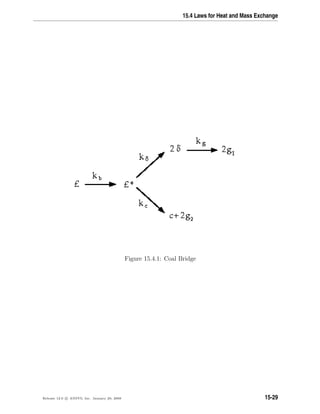
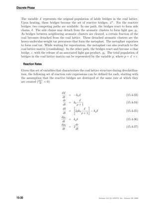
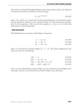
![Discrete Phase
Fractional Change in the Coal Mass
Given the set of reaction equations for the coal structure parameters, it is necessary to
relate these quantities to changes in coal mass and the related release of volatile products.
To accomplish this, the fractional change in the coal mass as a function of time is divided
into three parts: light gas (fgas), tar precursor fragments (ffrag), and char (fchar). This is
accomplished by using the following relationships, which are obtained using percolation
lattice statistics:
fgas(t) =
r(g1 + g2)(σ + 1)
4 + 2r(1 − c0)(σ + 1)
(15.4-46)
ffrag(t) =
2
2 + r(1 − c0)(σ + 1)
[ΦF(p) + rΩK(p)] (15.4-47)
fchar(t) = 1 − fgas(t) − ffrag(t) (15.4-48)
The variables Φ, Ω, F(p), and K(p) are the statistical relationships related to the cleaving
of bridges based on the percolation lattice statistics, and are given by the following
equations:
Φ = 1 + r
£
p
+
(σ − 1)δ
4(1 − p)
(15.4-49)
Ω =
δ
2(1 − p)
−
£
p
(15.4-50)
F(p) =
p
p
σ+1
σ−1
(15.4-51)
K(p) = 1 −
σ + 1
2
p
p
p
σ+1
σ−1
(15.4-52)
r is the ratio of bridge mass to site mass, mb/ma, where
mb = 2Mw,δ (15.4-53)
ma = Mw,1 − (σ + 1)Mw,δ (15.4-54)
15-32 Release 12.0 c ANSYS, Inc. January 29, 2009](https://image.slidesharecdn.com/flth-130501182911-phpapp02/85/Flth-464-320.jpg)
![15.4 Laws for Heat and Mass Exchange
where Mw,δ and Mw,1 are the side chain and cluster molecular weights respectively. σ +1
is the lattice coordination number, which is determined from solid-state nuclear magnetic
Resonance (NMR) measurements related to coal structure parameters, and p is the root
of the following equation in p (the total number of bridges in the coal lattice matrix):
p (1 − p )σ−1
= p(1 − p)σ−1
(15.4-55)
In accounting for mass in the metaplast (tar precursor fragments), the part that vaporizes
is treated in a manner similar to flash vaporization, where it is assumed that the finite
fragments undergo vapor/liquid phase equilibration on a time scale that is rapid with
respect to the bridge reactions. As an estimate of the vapor/liquid that is present at
any time, a vapor pressure correlation based on a simple form of Raoult’s Law is used.
The vapor pressure treatment is largely responsible for predicting pressure-dependent
devolatilization yields. For the part of the metaplast that reattaches to the coal lattice,
a cross-linking rate expression given by the following equation is used:
dmcross
dt
= mfragAcrosse−(Ecross/RT)
(15.4-56)
where mcross is the amount of mass reattaching to the matrix, mfrag is the amount of
mass in the tar precursor fragments (metaplast), and Across and Ecross are rate expression
constants.
CPD Inputs
Given the set of equations and corresponding rate constants introduced for the CPD
model, the number of constants that must be defined to use the model is a primary
concern. For the relationships defined previously, it can be shown that the following
parameters are coal independent [100]:
• Ab, Eb, Eσb, Ag, Eg, and Eσg for the rate constants kb and kg
• Across, Ecross, and ρ
These constants are included in the submodel formulation and are not input or modified
during problem setup.
Release 12.0 c ANSYS, Inc. January 29, 2009 15-33](https://image.slidesharecdn.com/flth-130501182911-phpapp02/85/Flth-465-320.jpg)
![Discrete Phase
There are an additional five parameters that are coal-specific and must be specified during
the problem setup:
• initial fraction of bridges in the coal lattice, p0
• initial fraction of char bridges, c0
• lattice coordination number, σ + 1
• cluster molecular weight, Mw,1
• side chain molecular weight, Mw,δ
The first four of these are coal structure quantities that are obtained from NMR exper-
imental data. The last quantity, representing the char bridges that either exist in the
parent coal or are formed very early in the devolatilization process, is estimated based
on the coal rank. These quantities are entered in the Create/Edit Materials dialog box, as
described in Section 23.5.2: Description of the Properties in the separate User’s Guide.
Values for the coal-dependent parameters for a variety of coals are listed in Table 15.4.1.
Table 15.4.1: Chemical Structure Parameters for 13
C NMR for 13 Coals
Coal Type σ + 1 p0 Mw,1 Mw,δ c0
Zap (AR) 3.9 .63 277 40 .20
Wyodak (AR) 5.6 .55 410 42 .14
Utah (AR) 5.1 .49 359 36 0
Ill6 (AR) 5.0 .63 316 27 0
Pitt8 (AR) 4.5 .62 294 24 0
Stockton (AR) 4.8 .69 275 20 0
Freeport (AR) 5.3 .67 302 17 0
Pocahontas (AR) 4.4 .74 299 14 .20
Blue (Sandia) 5.0 .42 410 47 .15
Rose (AFR) 5.8 .57 459 48 .10
1443 (lignite, ACERC) 4.8 .59 297 36 .20
1488 (subbituminous, ACERC) 4.7 .54 310 37 .15
1468 (anthracite, ACERC) 4.7 .89 656 12 .25
AR refers to eight types of coal from the Argonne premium sample bank [329, 363]. Sandia refers to
the coal examined at Sandia National Laboratories [99]. AFR refers to coal examined at Advanced Fuel
Research. ACERC refers to three types of coal examined at the Advanced Combustion Engineering
Research Center.
15-34 Release 12.0 c ANSYS, Inc. January 29, 2009](https://image.slidesharecdn.com/flth-130501182911-phpapp02/85/Flth-466-320.jpg)
![15.4 Laws for Heat and Mass Exchange
Particle Swelling During Devolatilization
The particle diameter changes during devolatilization according to the swelling coefficient,
Csw, which is defined by you and applied in the following relationship:
dp
dp,0
= 1 + (Csw − 1)
(1 − fw,0)mp,0 − mp
fv,0(1 − fw,0)mp,0
(15.4-57)
where dp,0 = particle diameter at the start of devolatilization
dp = current particle diameter
The term (1−fw,0)mp,0−mp
fv,0(1−fw,0)mp,0
is the ratio of the mass that has been devolatilized to the total
volatile mass of the particle. This quantity approaches a value of 1.0 as the devolatiliza-
tion law is applied. When the swelling coefficient is equal to 1.0, the particle diameter
stays constant. When the swelling coefficient is equal to 2.0, the final particle diam-
eter doubles when all of the volatile component has vaporized, and when the swelling
coefficient is equal to 0.5 the final particle diameter is half of its initial diameter.
Heat Transfer to the Particle During Devolatilization
Heat transfer to the particle during the devolatilization process includes contributions
from convection, radiation (if active), and the heat consumed during devolatilization:
mpcp
dTp
dt
= hAp(T∞ − Tp) +
dmp
dt
hfg + Ap pσ(θR
4
− Tp
4
) (15.4-58)
Radiation heat transfer to the particle is included only if you have enabled the P-1 or
discrete ordinates radiation model and you have activated radiation heat transfer to
particles using the Particle Radiation Interaction option in the Discrete Phase Model
dialog box.
By default, Equation 15.4-58 is solved analytically, by assuming that the temperature
and mass of the particle do not change significantly between time steps:
Tp(t + ∆t) = αp + [Tp(t) − αp]e−βp∆t
(15.4-59)
where
αp =
hApT∞ + dmp
dt
hfg + Ap pσθR
4
hAp + pApσTp
3 (15.4-60)
and
Release 12.0 c ANSYS, Inc. January 29, 2009 15-35](https://image.slidesharecdn.com/flth-130501182911-phpapp02/85/Flth-467-320.jpg)
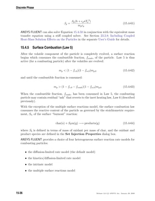
![15.4 Laws for Heat and Mass Exchange
Each of these models is described in detail below. You will choose the surface combustion
model when you are setting physical properties for the combusting-particle material, as
described in Section 23.5.2: Description of the Properties in the separate User’s Guide.
By default, the diffusion-limited rate model will be used.
The Diffusion-Limited Surface Reaction Rate Model
The diffusion-limited surface reaction rate model which is the default model in ANSYS
FLUENT, assumes that the surface reaction proceeds at a rate determined by the diffusion
of the gaseous oxidant to the surface of the particle:
dmp
dt
= −4πdpDi,m
YoxT∞ρ
Sb(Tp + T∞)
(15.4-65)
where Di,m = diffusion coefficient for oxidant in the bulk (m2
/s)
Yox = local mass fraction of oxidant in the gas
ρ = gas density (kg/m3
)
Sb = stoichiometry of Equation 15.4-64
Equation 15.4-65 is derived from the model of Baum and Street [20] with the kinetic con-
tribution to the surface reaction rate ignored. The diffusion-limited rate model assumes
that the diameter of the particles does not change. Since the mass of the particles is
decreasing, the effective density decreases, and the char particles become more porous.
The Kinetic/Diffusion Surface Reaction Rate Model
The kinetic/diffusion-limited rate model assumes that the surface reaction rate is deter-
mined either by kinetics or by a diffusion rate. ANSYS FLUENT uses the model of Baum
and Street [20] and Field [96], in which a diffusion rate coefficient
D0 = C1
[(Tp + T∞)/2]0.75
dp
(15.4-66)
and a kinetic rate
R = C2e−(E/RTp)
(15.4-67)
are weighted to yield a char combustion rate of
dmp
dt
= −Appox
D0R
D0 + R
(15.4-68)
Release 12.0 c ANSYS, Inc. January 29, 2009 15-37](https://image.slidesharecdn.com/flth-130501182911-phpapp02/85/Flth-469-320.jpg)
![Discrete Phase
where Ap is the surface area of the droplet (πd2
p), pox is the partial pressure of oxidant
species in the gas surrounding the combusting particle, and the kinetic rate, R, incorpo-
rates the effects of chemical reaction on the internal surface of the char particle (intrinsic
reaction) and pore diffusion. In ANSYS FLUENT, Equation 15.4-68 is recast in terms of
the oxidant mass fraction, Yox, as
dmp
dt
= −Ap
ρRT∞Yox
Mw,ox
D0R
D0 + R
(15.4-69)
The particle size is assumed to remain constant in this model while the density is allowed
to decrease.
When this model is enabled, the rate constants used in Equations 15.4-66 and 15.4-67 are
entered in the Create/Edit Materials dialog box, as described in Section 23.5: Setting
Material Properties for the Discrete Phase in the separate User’s Guide.
The Intrinsic Model
The intrinsic model in ANSYS FLUENT is based on Smith’s model [324], assuming the
order of reaction is equal to unity. Like the kinetic/diffusion model, the intrinsic model
assumes that the surface reaction rate includes the effects of both bulk diffusion and
chemical reaction (see Equation 15.4-69). The intrinsic model uses Equation 15.4-66 to
compute the diffusion rate coefficient, D0, but the chemical rate, R, is explicitly expressed
in terms of the intrinsic chemical and pore diffusion rates:
R = η
dp
6
ρpAgki (15.4-70)
η is the effectiveness factor, or the ratio of the actual combustion rate to the rate attain-
able if no pore diffusion resistance existed [182]:
η =
3
φ2
(φ coth φ − 1) (15.4-71)
where φ is the Thiele modulus:
φ =
dp
2
SbρpAgkipox
Deρox
1/2
(15.4-72)
15-38 Release 12.0 c ANSYS, Inc. January 29, 2009](https://image.slidesharecdn.com/flth-130501182911-phpapp02/85/Flth-470-320.jpg)
![15.4 Laws for Heat and Mass Exchange
ρox is the density of oxidant in the bulk gas (kg/m3
) and De is the effective diffusion
coefficient in the particle pores. Assuming that the pore size distribution is unimodal
and the bulk and Knudsen diffusion proceed in parallel, De is given by
De =
θ
τ2
1
DKn
+
1
D0
−1
(15.4-73)
where D0 is the bulk molecular diffusion coefficient and θ is the porosity of the char
particle:
θ = 1 −
ρp
ρt
(15.4-74)
ρp and ρt are, respectively, the apparent and true densities of the pyrolysis char.
τ (in Equation 15.4-73) is the tortuosity of the pores. The default value for τ in ANSYS
FLUENT is
√
2, which corresponds to an average intersecting angle between the pores
and the external surface of 45◦
[182].
DKn is the Knudsen diffusion coefficient:
DKn = 97.0rp
Tp
Mw,ox
(15.4-75)
where Tp is the particle temperature and rp is the mean pore radius of the char parti-
cle, which can be measured by mercury porosimetry. Note that macropores (rp 150
˚A) dominate in low-rank chars while micropores (rp 10 ˚A) dominate in high-rank
chars [182].
Ag (in Equations 15.4-70 and 15.4-72) is the specific internal surface area of the char
particle, which is assumed in this model to remain constant during char combustion.
Internal surface area data for various pyrolysis chars can be found in [323]. The mean
value of the internal surface area during char combustion is higher than that of the
pyrolysis char [182]. For example, an estimated mean value for bituminous chars is 300
m2
/g [50].
ki (in Equations 15.4-70 and 15.4-72) is the intrinsic reactivity, which is of Arrhenius
form:
ki = Aie−(Ei/RTp)
(15.4-76)
where the pre-exponential factor Ai and the activation energy Ei can be measured for
each char. In the absence of such measurements, the default values provided by ANSYS
FLUENT (which are taken from a least squares fit of data of a wide range of porous
carbons, including chars [323]) can be used.
Release 12.0 c ANSYS, Inc. January 29, 2009 15-39](https://image.slidesharecdn.com/flth-130501182911-phpapp02/85/Flth-471-320.jpg)
![Discrete Phase
To allow a more adequate description of the char particle size (and hence density) vari-
ation during combustion, you can specify the burning mode α, relating the char particle
diameter to the fractional degree of burnout U (where U = 1 − mp/mp,0) by [322]
dp
dp,0
= (1 − U)α
(15.4-77)
where mp is the char particle mass and the subscript zero refers to initial conditions (i.e.,
at the start of char combustion). Note that 0 ≤ α ≤ 1/3 where the limiting values 0 and
1/3 correspond, respectively, to a constant size with decreasing density (zone 1) and a
decreasing size with constant density (zone 3) during burnout. In zone 2, an intermediate
value of α = 0.25, corresponding to a decrease of both size and density, has been found
to work well for a variety of chars [322].
When this model is enabled, the rate constants used in Equations 15.4-66, 15.4-70,
15.4-72, 15.4-73, 15.4-75, 15.4-76, and 15.4-77 are entered in the Create/Edit Materi-
als dialog box, as described in Section 23.5: Setting Material Properties for the Discrete
Phase in the separate User’s Guide.
The Multiple Surface Reactions Model
Modeling multiple particle surface reactions follows a pattern similar to the wall surface
reaction models, where the surface species is now a “particle surface species”. For the
mixture material defined in the Species Model dialog box, the particle surface species can
be depleted or produced by the stoichiometry of the particle surface reaction (defined in
the Reactions dialog box). The particle surface species constitutes the reactive char mass
of the particle, hence, if a particle surface species is depleted, the reactive “char” content
of the particle is consumed, and in turn, when a surface species is produced, it is added
to the particle “char” mass. Any number of particle surface species and any number of
particle surface reactions can be defined for any given combusting particle.
Multiple injections can be accommodated, and combusting particles reacting according
to the multiple surface reactions model can coexist in the calculation, with combusting
particles following other char combustion laws. The model is based on oxidation studies
of char particles, but it is also applicable to gas-solid reactions in general, not only to
char oxidation reactions.
See Section 7.3: Particle Surface Reactions for information about particle surface reac-
tions.
15-40 Release 12.0 c ANSYS, Inc. January 29, 2009](https://image.slidesharecdn.com/flth-130501182911-phpapp02/85/Flth-472-320.jpg)
![15.4 Laws for Heat and Mass Exchange
Limitations
Note the following limitations of the multiple surface reactions model:
• The model is not available together with the unsteady tracking option.
• The model is available only with the species transport model for volumetric reac-
tions, and not with the nonpremixed, premixed, or partially premixed combustion
models.
Heat and Mass Transfer During Char Combustion
The surface reaction consumes the oxidant species in the gas phase; i.e., it supplies a
(negative) source term during the computation of the transport equation for this species.
Similarly, the surface reaction is a source of species in the gas phase: the product of
the heterogeneous surface reaction appears in the gas phase as a user-selected chemical
species. The surface reaction also consumes or produces energy, in an amount determined
by the heat of reaction defined by you.
The particle heat balance during surface reaction is
mpcp
dTp
dt
= hAp(T∞ − Tp) − fh
dmp
dt
Hreac + Ap pσ(θR
4
− Tp
4
) (15.4-78)
where Hreac is the heat released by the surface reaction. Note that only a portion (1−fh)
of the energy produced by the surface reaction appears as a heat source in the gas-
phase energy equation: the particle absorbs a fraction fh of this heat directly. For coal
combustion, it is recommended that fh be set to 1.0 if the char burnout product is CO
and 0.3 if the char burnout product is CO2 [33].
Radiation heat transfer to the particle is included only if you have enabled the P-1 or
discrete ordinates radiation model and you have activated radiation heat transfer to
particles using the Particle Radiation Interaction option in the Discrete Phase Model
dialog box.
By default, Equation 15.4-78 is solved analytically, by assuming that the temperature
and mass of the particle do not change significantly between time steps. ANSYS FLUENT
can also solve Equation 15.4-78 in conjunction with the equivalent mass transfer equation
using a stiff coupled solver. See Section 23.2.8: Including Coupled Heat-Mass Solution
Effects on the Particles in the separate User’s Guide for details.
Release 12.0 c ANSYS, Inc. January 29, 2009 15-41](https://image.slidesharecdn.com/flth-130501182911-phpapp02/85/Flth-473-320.jpg)
![15.5 Vapor Liquid Equilibrium Theory
Peng-Robinson Real Gas Model
For the calculation of the vapor concentration of a species Ci,S over the surface depends
on whether the compressability of the vapor phase ZV
is taken into account:
Ci,S = xi
V p
ZV RT
(15.4-84)
The data for the vapor pressure are no longer available, when a droplet material is chosen
as the component of a mixture, because it is not necessary for the calculation.
Besides using Raoult’s Law and the Peng-Robinson equation of state, you can define your
own user-defined function for delivering the vapor concentration at the particle surface .
For more information, see Section 2.5.15: DEFINE DPM VP EQUILIB in the separate UDF
Manual.
15.5 Vapor Liquid Equilibrium Theory
A number of industrially important processes, such as distillation, absorption and ex-
traction, bring into contact two phases which are not at equilibrium. The rate at which
a species is transferred from one phase to the other depends on the departure of the
system from equilibrium. The quantitative treatment of these rate processes requires
knowledge of the equilibrium states of the system. Apart from these cases, vapor-liquid
equilibrium (VLE) relationships in multicomponent systems are needed for the solution
of many other classes of engineering problems, such as the computation of evaporation
rates in spray combustion applications.
In ANSYS FLUENT the rate of vaporization of a single component droplet is computed
from Equation 15.4-12, where Ci,s is the equilibrium concentration of the droplet species
in the gas phase, and is computed in Equation 15.4-13 as:
Ci,s = psat/RTp (15.5-1)
where Tp is the droplet temperature, and psat is the saturation pressure of the droplet
species at Tp.
For the general case where N components are evaporating from a droplet (distillation),
the evaporation rate of each species is again given by Equation 15.4-12; however, psat in
Equation 15.5-1 must be replaced by pi, the partial pressure of species i, to calculate the
concentration of i at the droplet surface.
The partial pressure of species i can be obtained from the general expression for two phase
equilibrium, equating the fugacity of the liquid and vapor mixture components [275]:
fi
V
= xi
V
φi
V
p = xi
L
φi
L
p = fi
L
(15.5-2)
Release 12.0 c ANSYS, Inc. January 29, 2009 15-43](https://image.slidesharecdn.com/flth-130501182911-phpapp02/85/Flth-475-320.jpg)
![Discrete Phase
where xi is the mole fraction, φi is the fugacity coefficient for the species i in the mixture,
and p is the absolute pressure. The superscripts V and L are the vapor and the liquid
phase variables, respectively. The fugacity coefficients account for the nonideality in the
gas and liquid mixture. The fugacity of the liquid phase can be calculated from the pure
component’s saturation pressure psat,i [325]:
fi
L
= xi
L
φi
L
p = γixL
i φsat,i
L
psat,iexp
Vi
L
(p − psat,i)
RT
(15.5-3)
Here, φsat,i
L
is the fugacity coefficient for pure i at the saturation pressure; γi is the activ-
ity coefficient for species i in the mixture, and accounts for the nonideality in the liquid
phase; T is the particle surface temperature. We assume perfect thermal conductivity
inside the particle, so the particle temperature is used instead; R is the universal gas
constant; Vi
L
is the molar volume of the liquid. The exponential term is the Poynting
correction factor and accounts for the compressibility effects within the liquid. Except at
high pressures, the Poynting factor is usually negligible. Under low pressure conditions
where the gas phase may be assumed to be ideal, φi
V
≈ 1 and φsat,i ≈ 1 . Furthermore,
if the liquid is also assumed to be ideal, γ ≈ 1, then Equation 15.5-2 reduces to Raoult’s
law,
xi
V
p = xi
L
psat,i (15.5-4)
Raoult’s law is the default vapor-liquid equilibrium expression used in the ANSYS FLU-
ENT multicomponent droplet model. However, there is a UDF hook available for user-
defined vapor-liquid equilibrium models.
While Raoult’s law represents the simplest form of the VLE equation, keep in mind that
it is of limited use, as the assumptions made for its derivation are usually unrealistic.
The most critical assumption is that the liquid phase is an ideal solution. This is not
likely to be valid, unless the system is made up of species of similar molecular sizes and
chemical nature, such as in the case of benzene and toluene, or n-heptane and n-hexane.
When Raoult’s law is applicable, the vaporization rate of each species from a multicompo-
nent droplet can be computed from Equation 15.4-12, with the equilibrium concentration
of species i in the gas phase Ci,s computed as:
Ci,s = xipsat,i/RTp (15.5-5)
where Tp is the droplet temperature, xi is the mole fraction of species i in the droplet,
and psat,i is the saturation pressure of species i at Tp.
For higher pressures, especially near or above the critical point of the components, real
gas effects must be considered. Most models describing the fugacity coefficients use a
cubic equation of state with the general form:
15-44 Release 12.0 c ANSYS, Inc. January 29, 2009](https://image.slidesharecdn.com/flth-130501182911-phpapp02/85/Flth-476-320.jpg)
![15.5 Vapor Liquid Equilibrium Theory
p =
RT
V − b
−
a(V − η)
(V − b)(V 2 + δV − )
(15.5-6)
where V is the molar volume. For in-cylinder applications, the Peng-Robinson equation
of state is often used [265], where δ = 2b, = −b2
, and η = b:
p =
RT
V − b
−
a
V 2 + 2bV − b2
(15.5-7)
This equation defines the compressibility
Z =
pV
RT
=
RT
V − b
−
aV/RT
V 2 + 2bV − b2
(15.5-8)
The implementation of the Peng-Robinson equation of state in ANSYS FLUENT uses this
expression for both phases, the particle liquid and the vapor phase. The parameters a
and b are determined by the composition using a simple mixing law:
a =
N
i=1
N
j=1
xixj
√
aiaj
b =
N
i=1
xibi (15.5-9)
where N is the number of components in the mixture. The pure component parameters
can be obtained using the relationship with the Peng-Robinson constants:
ai = 4.57235
R2
T2
c,i
pc,i
1 + (0.480 + 1.574ωi − 0.176ωi
2
) 1 −
T
Tc,i
1/2
2
bi = 0.077796
RTc,i
Pc,i
(15.5-10)
where Tc,i is the critical temperature, pc,i is the critical pressure and ωi is the accentric
factor of the component i.
The fugacities of the components depend on the compressibility of the liquid and vapor
phase:
lnφi =
∂(Aγ
/RT)
∂Ni T,V,Nj=i
− lnZ (15.5-11)
Release 12.0 c ANSYS, Inc. January 29, 2009 15-45](https://image.slidesharecdn.com/flth-130501182911-phpapp02/85/Flth-477-320.jpg)
![Discrete Phase
where Aγ
is the residual Helmholtz energy, which is a function of the compressibility:
Aγ
RT
=
∞
V
[1 − Z]
dV
V
+ lnZ (15.5-12)
In summary, the vapor mole fraction xi
V
, the pressure p, and the compressibilities of the
vapor (ZV
) and the liquid (ZL
) phase at the surface of the particle are determined from
the liquid particle mole fraction of the components xi
L
and the particle temperature Tp.
The surface vapor concentrations are calculated using the following equation:
Ci,S = xi
V p
ZV RT
(15.5-13)
15.6 Wall-Jet Model Theory
The direction and velocity of the droplet particles are given by the resulting momen-
tum flux, which is a function of the impingement angle, φ, and Weber number. See
Figure 15.6.1.
x
z
φ
H(Ψ)
y
x
Ψ
side view top view
Figure 15.6.1: “Wall Jet” Boundary Condition for the Discrete Phase
The wall-jet type boundary condition assumes an analogy with an inviscid jet impacting
a solid wall. Equation 15.6-1 shows the analytical solution for an axisymmetric impinge-
ment assuming an empirical function for the sheet height (H) as a function of the angle
that the drop leaves the impingement (Ψ).
H(Ψ) = Hπeβ(1− Ψ
π
)
(15.6-1)
where Hπ is the sheet height at Ψ = π and β is a constant determined from conservation
of mass and momentum. The probability that a drop leaves the impingement point at
an angle between Ψ and Ψ + δΨ is given by integrating the expression for H(Ψ)
15-46 Release 12.0 c ANSYS, Inc. January 29, 2009](https://image.slidesharecdn.com/flth-130501182911-phpapp02/85/Flth-478-320.jpg)
![15.7 Wall-Film Model Theory
Ψ = −
π
β
ln[1 − P(1 − e−β
)] (15.6-2)
where P is a random number between 0 and 1. The expression for β is given in Naber
and Reitz [244] as
sin(φ) =
eβ
+ 1
(eβ − 1)(1 + (π
β
)2)
(15.6-3)
15.7 Wall-Film Model Theory
This section is composed of the following:
• Section 15.7.1: Introduction
• Section 15.7.2: Interaction During Impact with a Boundary
• Section 15.7.3: Splashing
• Section 15.7.4: Separation Criteria
• Section 15.7.5: Conservation Equations for Wall-Film Particles
15.7.1 Introduction
ANSYS FLUENT has a specific boundary condition for simulation of internal combustion
engines, called the wall-film model.
Spray-wall interaction is an important part of the mixture formation process in port fuel
injected (PFI) engines. A fuel spray impinges on a surface, usually at the intake port near
the intake valve, as well as at the intake valve itself, where it splashes and subsequently
evaporates. The evaporated mixture is entrained into the cylinder of the engine, where
it is mixed with the fresh charge and any residual gas in the cylinder. The mixture that
is compressed and burned, finally exits through the exhaust port. The process repeats
itself between 200 and 8000 times per minute, depending on the engine.
Several cycles worth of fuel remain in the intake tract due to film formation on the
walls. This in turn makes the film important in hydrocarbon emissions for PFI engines.
Additionally, film can form inside combustion chambers of direct injection (DI) types
of engines. In a direct injection engine, fuel is injected directly into the combustion
chamber, where the spray can impinge upon the piston if the injection event is early or
late in the cycle. The modeling of the wall-film inside a DI engine, especially in diesel
engines, is compounded by the presence of carbon deposits on the surfaces of the engine.
This carbon deposit absorbs the liquid film as it impinges upon it. It is believed that
Release 12.0 c ANSYS, Inc. January 29, 2009 15-47](https://image.slidesharecdn.com/flth-130501182911-phpapp02/85/Flth-479-320.jpg)
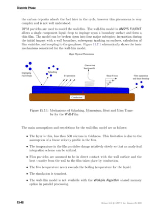
![15.7 Wall-Film Model Theory
If you wish to model a spray impacting a very hot wall, the wall-jet model may be
more appropriate as the assumption in the wall-jet impingement model is that there is
a vapor layer underneath the drops which keeps them from making direct contact with
the boundary surface. This may be a more accurate assumption for in-cylinder diesel
computations at typical operating conditions.
15.7.2 Interaction During Impact with a Boundary
The wall interaction is based on the work of Stanton [336] and O’Rourke [258], where
the regimes are calculated for a drop-wall interaction based on local information. The
four regimes, stick, rebound, spread, and splash are based on the impact energy and wall
temperature. The following chart is helpful in showing the cutoffs.
E
T
Tb Tw
E
Stick
Spread
Rebound
Splash
Figure 15.7.2: Simplified Decision Chart for Wall Interaction Criterion.
Below the boiling temperature of the liquid, the impinging droplet can either stick, spread
or splash, while above the boiling temperature, the particle can either rebound or splash.
The criteria by which the regimes are partitioned are based on the impact energy and
the boiling temperature of the liquid. The impact energy is defined by
E2
=
ρV 2
r D
σ
1
min (h0/D, 1) + δbl/D
(15.7-1)
where ρ is the liquid density, Vr is the relative velocity of the particle in the frame of the
wall (i.e. V 2
r = (Vp −Vw)2
), D is the diameter of the droplet, and σ is the surface tension
of the liquid. Here, δbl is a boundary layer thickness, defined by
δbl =
D
√
Re
(15.7-2)
where the Reynolds number is defined as Re = ρVrD/µ. By defining the energy as in
Equation 15.7-1, the presence of the film on the wall suppresses the splash, but does not
give unphysical results when the film height approaches zero.
Release 12.0 c ANSYS, Inc. January 29, 2009 15-49](https://image.slidesharecdn.com/flth-130501182911-phpapp02/85/Flth-481-320.jpg)
![Discrete Phase
The sticking regime is applied when the dimensionless energy E is less than 16, and the
particle velocity is set equal to the wall velocity. In the spreading regime, the initial di-
rection and velocity of the particle are set using the wall-jet model, where the probability
of the drop having a particular direction along the surface is given by an analogy of an
inviscid liquid jet with an empirically defined radial dependence for the momentum flux.
If the wall temperature is above the boiling temperature of the liquid, impingement events
below a critical impact energy (Ecr) results in the particles rebounding from the wall. For
the rebound regime, the particle rebounds with the following coefficient of restitution:
e = 0.993 − 1.76ΘI + 1.56Θ2
I − 0.49Θ3
I (15.7-3)
where ΘI is the impingement angle as measured from the wall surface.
Splashing occurs when the impingement energy is above a critical energy threshold,
defined as Ecr = 57.7. The number of splashed droplet parcels is set in the Wall boundary
condition dialog box with a default number of 4, however, you can select numbers between
zero and ten. The splashing algorithm follows that described by Stanton [336] and is
detailed in Section 15.7.3: Splashing.
15.7.3 Splashing
If the particle impinging on the surface has a sufficiently high energy, the particle splashes
and several new particles are created. You can explicitly set the number of particles cre-
ated by each impact in the DPM tab of the Wall boundary condition dialog box. The
number of splashed parcels may be set to an integer value between zero and ten. The
properties (diameter, magnitude, and direction) of the splashed parcels are randomly
sampled from the experimentally obtained distribution functions described in the fol-
lowing sections. Setting the number of splashed parcels to zero turns off the splashing
calculation. Bear in mind that each splashed parcel can be considered a discrete sample
of the distribution curves and that selecting the number of splashed drops in the Wall
boundary condition dialog box does not limit the number of splashed drops, only the
number of parcels representing those drops.
Therefore, for each splashed parcel, a different diameter is obtained by sampling a cu-
mulative probability distribution function (CPDF), which is obtained from a Weibull
distribution function and fitted to the data from Mundo, et al. [241]. The equation is
pdf
d
D
= 2
d
D2
exp
−
d
D
2
(15.7-4)
and it represents the probability of finding drops of diameter di in a sample of splashed
drops. This distribution is similar to the Nakamura-Tanasawa distribution function used
by O’Rourke [258], but with the peak of the distribution function being D = dmax/
√
2.
To ensure that the distribution functions produce physical results with an increasing
15-50 Release 12.0 c ANSYS, Inc. January 29, 2009](https://image.slidesharecdn.com/flth-130501182911-phpapp02/85/Flth-482-320.jpg)
![15.7 Wall-Film Model Theory
Weber number, the following expression for dmax from O’Rourke [258] is used. The peak
of the splashed diameter distribution is
dmax/d0 = MAX
E2
crit
E2
,
6.4
We
, 0.06 (15.7-5)
where the expression for energy is given by Equation 15.7-1. Low Weber number impacts
are described by the second term in Equation 15.7-5 and the peak of the minimum
splashed diameter distribution is never less than 0.06 for very high energy impacts in any
of the experiments analyzed by O’Rourke [258]. The Weber number in Equation 15.7-5
is defined using the relative velocity and drop diameter:
We =
ρV 2
r D
σ
(15.7-6)
The cumulative probability distribution function (CPDF) is needed so that a diameter
can be sampled from the experimental data. The CPDF is obtained from integrating
Equation 15.7-4 to obtain
cpdf
d
D
= 1 − exp
−
d
D
2
(15.7-7)
which is bounded by zero and one. An expression for the diameter (which is a function
of D, the impingement Weber number We, and the impingement energy) is obtained by
inverting Equation 15.7-7 and sampling the CPDF between zero and one. The expression
for the diameter of the ith
splashed parcel is therefore given by,
di = D − ln (1 − ci)
where ci is the ith
random sample. Once the diameter of the splashed drop has been
determined, the probability of finding that drop in a given sample is determined by
evaluating Equation 15.7-4 at the given diameter. The number of drops per parcel can
be expressed as a function of the total number of splashed drops:
Ni = Ntotpdfi (15.7-8)
where the pdfi is for the ith
sample. The values of pdfi are then normalized so that their
sum is one. Both the number per parcel (Ni) and the total number of splashed drops
(Ntot) is unknown, but an expression for Ntot can be obtained from the conservation of
mass if the total splashed mass is known.
The amount of mass splashed from the surface is a quadratic function of the splashing
energy, obtained from the experimental data from Mundo [241]. The splashed mass
fraction ys is given by
ys =
1.8x10⁻⁴
(E2
− E2
crit) , E2
crit E2
7500
0.70 , E2
7500
Release 12.0 c ANSYS, Inc. January 29, 2009 15-51](https://image.slidesharecdn.com/flth-130501182911-phpapp02/85/Flth-483-320.jpg)
![Discrete Phase
The authors (O’Rourke et al. [258]) noted that nearly all of the impacts for typical diesel
sprays are well above the upper bound and so the splashing event nearly always ejects
70% of the mass of the impinging drop. To obtain an expression for the total number of
drops, we note that overall conservation of mass requires that the sum of the total mass
of the splashed parcel(s) must equal the splashed mass fraction, or
ρπ
6
Ntot
Nparcels
n=1
pdfnd3
n = ysm0 (15.7-9)
where m0 is the total mass of the impinging parcel. The expression for the total number
of splashed drops is
Ntot =
ysm0
ρπ
6
Nparcels
n=1 (pdfnd3
n)
The number of splashed drops per parcel is then determined by Equation 15.7-8 with the
values of pdfi given by Equation 15.7-4.
To calculate the velocity with which the splashed drops leave the surface, additional
correlations are sampled for the normal component of the velocity. A Weibull function,
fit to the data from Mundo [241], is used as the PDF for the normal component. The
probability density is given by
pdf
Vni
Vnd
=
bv
Θv
Vni/Vnd
Θv
bv−1
exp
−
Vni/Vnd
Θv
bv
(15.7-10)
where
bv =
2.1, ΘI ≤ 50◦
1.10 + 0.02ΘI, ΘI 50◦ (15.7-11)
and
Θv = 0.158e0.017ΘI
(15.7-12)
where ΘI is the angle at which the parcel impacts the surface, or the impingement angle.
The tangential component of the velocity is obtained from the expression for the reflection
angle Θs:
Θs = 65.4 + 0.226Θl (15.7-13)
combined with
Vti =
Vni
tan(Θs)
(15.7-14)
Finally, an energy balance is performed for the new parcels so that the sum of the kinetic
and surface energies of the new drops does not exceed that of the old drops. The energy
balance is given by
1
2
Nparcel
i=1
miV 2
i + πσ
Nparcel
i=1
Nid2
i =
1
2
mdV 2
d miV 2
i + πσ mdd2
i − Ecrit
15-52 Release 12.0 c ANSYS, Inc. January 29, 2009](https://image.slidesharecdn.com/flth-130501182911-phpapp02/85/Flth-484-320.jpg)
![15.7 Wall-Film Model Theory
where Ecrit is the threshold energy for splashing to occur. To ensure conservation of
energy, the following correction factor is computed:
K =
1
2
mdV 2
d (miV 2
i ) + πσ (mdd2
i ) − Ecrit − πσ
Nparcel
i=1 (Nid2
i )
1
2
Nparcel
i=1 (miV 2
i )
. (15.7-15)
This correction factor is needed due to the relatively small number of sampled points for
the velocity of the splashed drops (see Stanton [337] for more detail). The components
of the splashed parcel are multiplied by the square root of K in Equation 15.7-15 so that
energy will be conserved. The normal and tangential velocity components of the splashed
parcels are therefore given by
Vni =
√
KVni and Vti =
√
KVti
ANSYS FLUENT will limit the velocity of the splashed parcels so that they do not exceed
the impact velocity of the original parcel. It is important to note that splashing events are
inherently transient, so the splashing submodel is only available with unsteady tracking
in ANSYS FLUENT. Splashing can also cause large increases in source terms in the cells
in which it occurs, which can cause difficulty in convergence between time steps. Thus,
it may be necessary to use a smaller time step during the simulation when splashing is
enabled.
15.7.4 Separation Criteria
The film can separate from the wall when the stress at an edge of the film exceeds
the adhesion forces holding the film to the wall. These forces are complex and highly
dependent on local surface conditions. An order of magnitude analysis of a film rounding
a sharp corner shows that the stresses at the edge of a film are proportional to the angle
which the film negotiates. In ANSYS FLUENT, you can specify the maximum angle that
the film can negotiate using a special text command. For more information, contact your
ANSYS FLUENT support engineer.
Release 12.0 c ANSYS, Inc. January 29, 2009 15-53](https://image.slidesharecdn.com/flth-130501182911-phpapp02/85/Flth-485-320.jpg)
![Discrete Phase
15.7.5 Conservation Equations for Wall-Film Particles
Conservation equations for momentum, mass, and energy for individual parcels in the
wall-film are described below. The particle-based approach for thin films was first for-
mulated by O’Rourke [257] and most of the following derivation is based closely on that
work.
Momentum
The equation for the momentum of a parcel on the film is
ρh
dup
dt
+ h( spf )α = τgtg + τwtw +
˙
Pimp,α − ˙Mimp,αup +
˙
Fn,α + ρh(g − aw) (15.7-16)
where α denotes the current face on which the particle resides, h denotes the current film
height at the particle location, s is the gradient operator restricted to the surface, and
pf is the pressure on the surface of the film. On the right-hand side of Equation 15.7-16,
τg denotes the magnitude of the shear stress of the gas flow on the surface of the film, tg
is the unit vector in the direction of the relative motion of the gas and the film surface,
µl is the liquid viscosity, and τw is the magnitude of the stress that the wall exerts on
the film. Similarly to the expression for tg, tw is the unit vector in the direction of the
relative motion of the film and the wall. The remaining expressions on the right-hand
side of Equation 15.7-16 are
˙
Pimp,α which denotes the impingement pressure on the film
surface,
˙
Mimp,α is the impingement momentum source, and
˙
Fn,α is the force necessary
to keep the film on the surface, as determined by
up · ˆnα = 0. (15.7-17)
Here, ρh(g − aw) is the body force term. Note that the body force term can be very
significant, despite the small values of film thickness due to the very high acceleration
rates seen in simulations with moving boundaries. The requirement represented by Equa-
tion 15.7-17 is explicitly enforced at each time step in ANSYS FLUENT for all particles
representing the wall-film.
The term h( spf )α is the surface gradient of the pressure on the face, pf . This pressure,
pf , is the sum of the fluid pressure and the impingement pressure from the drops on the
face, given by
pf = Pcell −
˙
Pimp,α · ˆn + ˙Mimp,αup · ˆn
where the impingement mass ˙Mimp,α is given by
˙Mimp,α = ρlVpv · ˆnf(xs, v, r, Td, t)drdvdTd (15.7-18)
and the impingement pressure is given by
˙
Pimp,α = ρlVpvv · ˆnf(xs, v, r, Td, t)drdvdTd (15.7-19)
15-54 Release 12.0 c ANSYS, Inc. January 29, 2009](https://image.slidesharecdn.com/flth-130501182911-phpapp02/85/Flth-486-320.jpg)
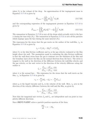
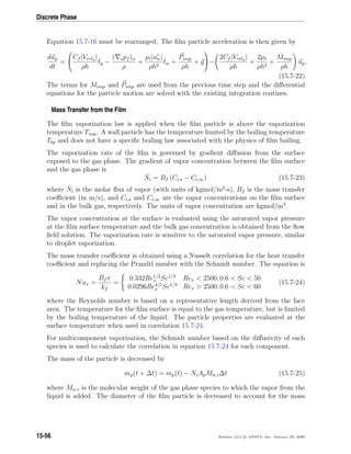
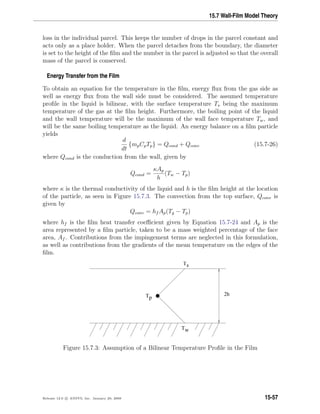
![Discrete Phase
Assuming that the temperature changes slowly for each particle in the film, the equation
for the change in temperature of a non vaporizing particle can be written as
mpCp
dTp
dt
= Ap − hf +
κ
h
Tp + hTg +
κ
h
Tw (15.7-27)
As the particle trajectory is computed, ANSYS FLUENT integrates Equation 15.7-27 to
obtain the particle temperature at the next time value, yielding
Tp(t + ∆t) = αp + [Tp(t) − αp]e−βp∆t
(15.7-28)
where ∆t is the integration time step and αp and βp are given by
αp =
hf Tg + κ
h
Tw
hf + κ
h
(15.7-29)
and
βp =
Ap(hf + κ
h
)
mpCp
(15.7-30)
When the particle changes its mass during vaporization, an additional term is added to
Equation 15.7-27 to account for the enthalpy of vaporization, which is given by
mpCp
dTp
dt
= Ap − hf +
κ
h
Tp + hTg +
κ
h
Tw + ˙mphfg (15.7-31)
where hfg is the latent heat of vaporization (with units of J/kg) and the expression ˙mp
is the rate of evaporation in kg/s. This alters the expression for αp in Equation 15.7-29
so that
αp =
hf Tg + κ
h
Tw + ˙mphfg/Ap
hf + κ
h
(15.7-32)
When the wall-film model is active, the heat flux from the wall to the liquid film is
subtracted from the heat flux from the wall to the gas phase. Additionally, enthalpy
from vaporization of the liquid from the wall is subtracted from the cell to which the
vapor mass goes. Since film boiling is modeled by limiting the liquid phase temperature
to the boiling point of the material, energy in excess of that absorbed by the liquid will
be put into the gas phase. When the thermal boundary conditions on the wall are set
to a constant heat flux, the local temperature of the wall face is used as the thermal
boundary condition for the wall-film particles.
i The wall-film model has been specifically implemented for in-cylinder flows
and should be used with caution for other applications.
15-58 Release 12.0 c ANSYS, Inc. January 29, 2009](https://image.slidesharecdn.com/flth-130501182911-phpapp02/85/Flth-490-320.jpg)
![15.8 Particle Erosion and Accretion Theory
15.8 Particle Erosion and Accretion Theory
Particle erosion and accretion rates can be monitored at wall boundaries. The erosion
rate is defined as
Rerosion =
Nparticles
p=1
˙mpC(dp)f(α)vb(v)
Aface
(15.8-1)
where C(dp) is a function of particle diameter, α is the impact angle of the particle path
with the wall face, f(α) is a function of impact angle, v is the relative particle velocity,
b(v) is a function of relative particle velocity, and Aface is the area of the cell face at the
wall. Default values are C = 1.8 × 10⁻⁹
, f = 1, and b = 0.
Since C, f, and b are defined as boundary conditions at a wall, rather than properties
of a material, the default values are not updated to reflect the material being used. You
will need to specify appropriate values at all walls. Values of these functions for sand
eroding both carbon steel and aluminum are given by Edwards et al. [86].
The erosion rate as calculated above is displayed in units of removed material/(area-
time), i.e., mass flux, and can therefore be changed accordingly to the defined units in
ANSYS FLUENT. The functions C and f have to be specified in consistent units to build
a dimensionless group with the relative particle velocity and its exponent. To compute
an erosion rate in terms of length/time (mm/year, for example) you can either define a
custom field function to divide the erosion rate by the density of the wall material or
include this division in the units for C and/or f. Note that the units given by ANSYS
FLUENT when displaying the erosion rate are no longer valid in the latter case.
A variety of erosion models [97, 221, 85, 249, 126, 299] containing model constants [126,
85] and angle functions can be easily implemented into ANSYS FLUENT. The equations
describing some of the erosion models can be modified to appear in the form of the
general equation describing the erosion rate, Equation 15.8-1. For example, the Tulsa
Angle Dependent Model [85] described by Equation 15.8-2
ER = 1559B−0.59
Fsv1.73
f(α) (15.8-2)
can be rewritten in the form of Equation 15.8-1 with the following substitutions:
v1.73
= vb(v)
1559B−0.59
Fs = C(dp)
where ER is the erosion rate, B is the Brinell hardness, and Fs is a particle shape
coefficient.
Release 12.0 c ANSYS, Inc. January 29, 2009 15-59](https://image.slidesharecdn.com/flth-130501182911-phpapp02/85/Flth-491-320.jpg)
![15.9 Atomizer Model Theory
Five atomizer models are available in ANSYS FLUENT to predict the spray characteristics
from knowledge of global parameters such as nozzle type and liquid flow rate. You can
choose them as injection types and define the associated parameters in the Set Injection
Properties dialog box, as described in Section 23.3.1: Injection Types in the separate
User’s Guide. Details about the atomizer models are provided below.
Information is organized into the following subsections:
• Section 15.9.1: The Plain-Orifice Atomizer Model
• Section 15.9.2: The Pressure-Swirl Atomizer Model
• Section 15.9.3: The Air-Blast/Air-Assist Atomizer Model
• Section 15.9.4: The Flat-Fan Atomizer Model
• Section 15.9.5: The Effervescent Atomizer Model
15.9.1 The Plain-Orifice Atomizer Model
The plain-orifice is the most common type of atomizer and the most simply made. How-
ever there is nothing simple about the physics of the internal nozzle flow and the external
atomization. In the plain-orifice atomizer model in ANSYS FLUENT, the liquid is accel-
erated through a nozzle, forms a liquid jet and then breaks up to form droplets. This
apparently simple process is dauntingly complex. The plain orifice may operate in three
different regimes: single-phase, cavitating and flipped [330]. The transition between
regimes is abrupt, producing dramatically different sprays. The internal regime deter-
mines the velocity at the orifice exit, as well as the initial droplet size and the angle of
droplet dispersion. Diagrams of each case are shown in Figures 15.9.1, 15.9.2, and 15.9.3.
Release 12.0 c ANSYS, Inc. January 29, 2009 15-61](https://image.slidesharecdn.com/flth-130501182911-phpapp02/85/Flth-493-320.jpg)
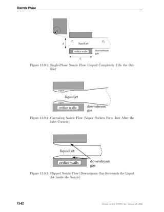
![15.9 Atomizer Model Theory
Internal Nozzle State
To accurately predict the spray characteristics, the plain-orifice model in ANSYS FLUENT
must identify the correct state of the internal nozzle flow because the nozzle state has
a tremendous effect on the external spray. Unfortunately, there is no established theory
for determining the nozzle state. One must rely on empirical models obtained from
experimental data. ANSYS FLUENT uses several dimensionless parameters to determine
the internal flow regime for the plain-orifice atomizer model. These parameters and the
decision-making process are summarized below.
A list of the parameters that control internal nozzle flow is given in Table 15.9.1. These
parameters may be combined to form nondimensional characteristic lengths such as r/d
and L/d, as well as nondimensional groups like the Reynolds number based on hydraulic
“head” (Reh) and the cavitation parameter (K).
Table 15.9.1: List of Governing Parameters for Internal Nozzle Flow
nozzle diameter d
nozzle length L
radius of curvature of the inlet corner r
upstream pressure p1
downstream pressure p2
viscosity µ
liquid density ρl
vapor pressure pv
Reh =
dρl
µ
2(p1 − p2)
ρl
(15.9-1)
K =
p1 − pv
p1 − p2
(15.9-2)
The liquid flow often contracts in the nozzle, as can be seen in Figures 15.9.2 and 15.9.3.
Nurick [252] found it helpful to use a coefficient of contraction (Cc) to represent the
reduction in the cross-sectional area of the liquid jet. The coefficient of contraction is
defined as the area of the stream of contracting liquid over the total cross-sectional area
of the nozzle. ANSYS FLUENT uses Nurick’s fit for the coefficient of contraction:
Cc =
1
1
C2
ct
− 11.4r
d
(15.9-3)
Release 12.0 c ANSYS, Inc. January 29, 2009 15-63](https://image.slidesharecdn.com/flth-130501182911-phpapp02/85/Flth-495-320.jpg)
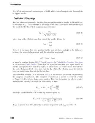
![15.9 Atomizer Model Theory
The cavitation number, K, is compared to the values of Kincep and Kcrit to identify the
nozzle state. The decision tree is shown in Figure 15.9.4. Depending on the state of the
nozzle, a unique closure is chosen for the above equations.
For a single-phase nozzle (K Kincep, K ≥ Kcrit) [193], the coefficient of discharge is
given by
Cd =
1
1
Cdu
+ 20(1+2.25L/d)
Reh
(15.9-9)
where Cdu is the ultimate discharge coefficient, and is defined as
Cdu = 0.827 − 0.0085
L
d
(15.9-10)
For a cavitating nozzle (Kcrit ≤ K ≤ Kincep) [252] the coefficient of discharge is deter-
mined from
Cd = Cc
√
K (15.9-11)
For a flipped nozzle (K Kcrit) [252],
Cd = Cct = 0.611 (15.9-12)
incep
crit
incep
crit crit crit
K KK ≤ K
K K K ≥ K K K K ≥ K
flipped cavitating flipped single phase
Figure 15.9.4: Decision Tree for the State of the Cavitating Nozzle
All of the nozzle flow equations are solved iteratively, along with the appropriate relation-
ship for coefficient of discharge as given by the nozzle state. The nozzle state may change
as the upstream or downstream pressures change. Once the nozzle state is determined,
the exit velocity is calculated, and appropriate correlations for spray angle and initial
droplet size distribution are determined.
Release 12.0 c ANSYS, Inc. January 29, 2009 15-65](https://image.slidesharecdn.com/flth-130501182911-phpapp02/85/Flth-497-320.jpg)
![Discrete Phase
Exit Velocity
For a single-phase nozzle, the estimate of exit velocity (u) comes from the conservation
of mass and the assumption of a uniform exit velocity:
u =
˙meff
ρlA
(15.9-13)
For the cavitating nozzle, Schmidt and Corradini [306] have shown that the uniform exit
velocity is not accurate. Instead, they derived an expression for a higher velocity over a
reduced area:
u =
2Ccp1 − p2 + (1 − 2Cc)pv
Cc 2ρl(p1 − pv)
(15.9-14)
This analytical relation is used for cavitating nozzles in ANSYS FLUENT. For the case of
flipped nozzles, the exit velocity is found from the conservation of mass and the value of
the reduced flow area:
u =
˙meff
ρlCctA
(15.9-15)
Spray Angle
The correlation for the spray angle (θ) comes from the work of Ranz [283]:
θ
2
=
tan−1 4π
CA
ρg
ρl
√
3
6
single phase, cavitating
0.01 flipped
(15.9-16)
The spray angle for both single-phase and cavitating nozzles depends on the ratio of the
gas and liquid densities and also the parameter CA. For flipped nozzles, the spray angle
has a constant value.
The parameter CA, which you must specify, is thought to be a constant for a given nozzle
geometry. The larger the value, the narrower the spray. Reitz [288] suggests the following
correlation for CA:
CA = 3 +
L
3.6d
(15.9-17)
15-66 Release 12.0 c ANSYS, Inc. January 29, 2009](https://image.slidesharecdn.com/flth-130501182911-phpapp02/85/Flth-498-320.jpg)
![15.9 Atomizer Model Theory
The spray angle is sensitive to the internal flow regime of the nozzle. Hence, you may
wish to choose smaller values of CA for cavitating nozzles than for single-phase nozzles.
Typical values range from 4.0 to 6.0. The spray angle for flipped nozzles is a small,
arbitrary value that represents the lack of any turbulence or initial disturbance from the
nozzle.
Droplet Diameter Distribution
One of the basic characteristics of an injection is the distribution of drop size. For an
atomizer, the droplet diameter distribution is closely related to the nozzle state. ANSYS
FLUENT’s spray models use a two-parameter Rosin-Rammler distribution, characterized
by the most probable droplet size and a spread parameter. The most probable droplet
size, d0 is obtained in ANSYS FLUENT from the Sauter mean diameter, d32 [186]. For
more information about the Rosin-Rammler size distribution, see Section 23.3.13: Using
the Rosin-Rammler Diameter Distribution Method in the separate User’s Guide.
For single-phase nozzle flows, the correlation of Wu et al. [383] is used to calculate d32
and relate the initial drop size to the estimated turbulence quantities of the liquid jet:
d32 = 133.0λWe−0.74
, (15.9-18)
where λ = d/8, λ is the radial integral length scale at the jet exit based upon fully-
developed turbulent pipe flow, and We is the Weber number, defined as
We ≡
ρlu2
λ
σ
. (15.9-19)
Here, σ is the droplet surface tension. For a more detailed discussion of droplet surface
tension and the Weber number, see Section 15.10: Secondary Breakup Model Theory. For
more information about mean particle diameters, see Section 23.7.8: Summary Reporting
of Current Particles in the separate User’s Guide.
For cavitating nozzles, ANSYS FLUENT uses a slight modification of Equation 15.9-18.
The initial jet diameter used in Wu’s correlation, d, is calculated from the effective area of
the cavitating orifice exit, and thus represents the effective diameter of the exiting liquid
jet, deff. For an explanation of effective area of cavitating nozzles, please see Schmidt
and Corradini [306].
The length scale for a cavitating nozzle is λ = deff/8, where
deff =
4 ˙meff
πρlu
. (15.9-20)
Release 12.0 c ANSYS, Inc. January 29, 2009 15-67](https://image.slidesharecdn.com/flth-130501182911-phpapp02/85/Flth-499-320.jpg)
![Discrete Phase
For the case of the flipped nozzle, the initial droplet diameter is set to the diameter of
the liquid jet:
d0 = d Cct (15.9-21)
where d0 is defined as the most probable diameter.
The second parameter required to specify the droplet size distribution is the spread
parameter, s. The values for the spread parameter are chosen from past modeling expe-
rience and from a review of experimental observations. Table 15.9.2 lists the values of s
for the three nozzle states. The larger the value of the spread parameter, the narrower
the droplet size distribution.
Table 15.9.2: Values of Spread Parameter for Different Nozzle States
State Spread Parameter
single phase 3.5
cavitating 1.5
flipped ∞
Since the correlations of Wu et al. provide the Sauter mean diameter, d32, these are
converted to the most probable diameter, d0. Lefebvre [186] gives the most general
relationship between the Sauter mean diameter and most probable diameter for a Rosin-
Rammler distribution. The simplified version for s=3.5 is as follows:
d0 = 1.2726d32 1 −
1
s
1/s
(15.9-22)
At this point, the droplet size, velocity, and spray angle have been determined and the
initialization of the injections is complete.
15-68 Release 12.0 c ANSYS, Inc. January 29, 2009](https://image.slidesharecdn.com/flth-130501182911-phpapp02/85/Flth-500-320.jpg)
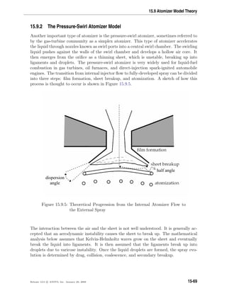
![Discrete Phase
The pressure-swirl atomizer model used in ANSYS FLUENT is called the Linearized In-
stability Sheet Atomization (LISA) model of Schmidt et al. [308]. The LISA model is
divided into two stages:
1. film formation
2. sheet breakup and atomization
Both parts of the model are described below.
Film Formation
The centrifugal motion of the liquid within the injector creates an air core surrounded
by a liquid film. The thickness of this film, t, is related to the mass flow rate by
˙meff = πρut(dinj − t) (15.9-23)
where dinj is the injector exit diameter, and ˙meff is the effective mass flow rate, which
is defined by Equation 15.9-5 . The other unknown in Equation 15.9-23 is u, the axial
component of velocity at the injector exit. This quantity depends on internal details
of the injector and is difficult to calculate from first principles. Instead, the approach
of Han et al. [122] is used. The total velocity is assumed to be related to the injector
pressure by
U = kv
2∆p
ρl
(15.9-24)
where kv is the velocity coefficient. Lefebvre [186] has noted that kv is a function of the
injector design and injection pressure. If the swirl ports are treated as nozzles and if it is
assumed that the dominant portion of the pressure drop occurs at those ports, kv is the
expression for the discharge coefficient (Cd). For single-phase nozzles with sharp inlet
corners and L/d ratios of 4, a typical Cd value is 0.78 or less [193]. If the nozzles are
cavitating, the value of Cd may be as low as 0.61. Hence, 0.78 should be a practical upper
bound for kv. Reducing kv by 10% to 0.7 approximates the effect of other momentum
losses on the discharge coefficient.
Physical limits on kv require that it be less than unity from conservation of energy, yet
be large enough to permit sufficient mass flow. To guarantee that the size of the air core
is non-negative, the following expression is used for kv:
kv = max 0.7,
4 ˙meff
d2
0ρl cos θ
ρl
2∆p
(15.9-25)
15-70 Release 12.0 c ANSYS, Inc. January 29, 2009](https://image.slidesharecdn.com/flth-130501182911-phpapp02/85/Flth-502-320.jpg)
![15.9 Atomizer Model Theory
Assuming that ∆p is known, Equation 15.9-24 can be used to find U. Once U is deter-
mined, u is found from
u = U cos θ (15.9-26)
where θ is the spray angle, which is assumed to be known. At this point, the thickness
and axial component of the liquid film are known at the injector exit. The tangential
component of velocity (w = U sin θ) is assumed to be equal to the radial velocity compo-
nent of the liquid sheet downstream of the nozzle exit. The axial component of velocity
is assumed to remain constant.
Sheet Breakup and Atomization
The pressure-swirl atomizer model includes the effects of the surrounding gas, liquid
viscosity, and surface tension on the breakup of the liquid sheet. Details of the theoretical
development of the model are given in Senecal et al. [310] and are only briefly presented
here. For a more robust implementation, the gas-phase velocity is neglected in calculating
the relative liquid-gas velocity and is instead set by you. This avoids having the injector
parameters depend too heavily on the usually under-resolved gas-phase velocity field very
near the injection location.
The model assumes that a two-dimensional, viscous, incompressible liquid sheet of thick-
ness 2h moves with velocity U through a quiescent, inviscid, incompressible gas medium.
The liquid and gas have densities of ρl and ρg, respectively, and the viscosity of the
liquid is µl. A coordinate system is used that moves with the sheet, and a spectrum of
infinitesimal wavy disturbances of the form
η = η0eikx+ωt
(15.9-27)
is imposed on the initially steady motion. The spectrum of disturbances results in fluc-
tuating velocities and pressures for both the liquid and the gas. In Equation 15.9-27, η0
is the initial wave amplitude, k = 2π/λ is the wave number, and ω = ωr + iωi is the
complex growth rate. The most unstable disturbance has the largest value of ωr, denoted
here by Ω, and is assumed to be responsible for sheet breakup. Thus, it is desired to
obtain a dispersion relation ω = ω(k) from which the most unstable disturbance can be
calculated as a function of wave number.
Squire [335], Li and Tankin [192], and Hagerty and Shea [118] have shown that two
solutions, or modes, exist that satisfy the governing equations subject to the boundary
conditions at the upper and lower interfaces. The first solution, called the sinuous mode,
has waves at the upper and lower interfaces in phase. The second solution is called the
varicose mode which has the waves at the upper and lower interfaces π radians out of
phase. It has been shown by numerous authors (e.g., Senecal et. al. [310]) that the
Release 12.0 c ANSYS, Inc. January 29, 2009 15-71](https://image.slidesharecdn.com/flth-130501182911-phpapp02/85/Flth-503-320.jpg)
![Discrete Phase
sinuous mode dominates the growth of varicose waves for low velocities and low gas-to-
liquid density ratios. In addition, it can be shown that the sinuous and varicose modes
become indistinguishable for high-velocity flows. As a result, the atomization model in
ANSYS FLUENT is based upon the growth of sinuous waves on the liquid sheet.
As derived in Senecal et al. [310], the dispersion relation for the sinuous mode is given
by
ω2
[tanh(kh) + Q] + [4νlk2
tanh(kh) + 2iQkU] +
4νlk4
tanh(kh) − 4ν2
l k3
tanh( h) − QU2
k2
+
σk3
ρl
= 0 (15.9-28)
where Q = ρg/ρl and 2
= k2
+ ω/νl.
Above a critical Weber number of Weg = 27/16 (based on the liquid velocity, gas density,
and sheet half-thickness), the fastest-growing waves are short. For Weg 27/16, the
wavelengths are long compared to the sheet thickness. The speed of modern high pressure
fuel injection systems is high enough to ensure that the film Weber number is well above
this critical limit.
An order-of-magnitude analysis using typical values shows that the terms of second order
in viscosity can be neglected in comparison to the other terms in Equation 15.9-28. Using
this assumption, Equation 15.9-28 reduces to
ωr =
1
tanh(kh) + Q
−2νlk2
tanh(kh) +
4ν2
l k4 tanh2
(kh) − Q2U2k2 − [tanh(kh) + Q] −QU2k2 +
σk3
ρl
(15.9-29)
For waves that are long compared with the sheet thickness, a mechanism of sheet disin-
tegration proposed by Dombrowski and Johns [74] is adopted. For long waves, ligaments
are assumed to form from the sheet breakup process once the unstable waves reach a
critical amplitude. If the surface disturbance has reached a value of ηb at breakup, a
breakup time, τ, can be evaluated:
ηb = η0eΩτ
⇒
1
Ω
ln
ηb
η0
(15.9-30)
where Ω, the maximum growth rate, is found by numerically maximizing Equation 15.9-29
as a function of k. The maximum is found using a binary search that checks the sign of
the derivative. The sheet breaks up and ligaments will be formed at a length given by
15-72 Release 12.0 c ANSYS, Inc. January 29, 2009](https://image.slidesharecdn.com/flth-130501182911-phpapp02/85/Flth-504-320.jpg)
![15.9 Atomizer Model Theory
Lb = Uτ =
U
Ω
ln
ηb
η0
(15.9-31)
where the quantity ln(ηb
η0
) is an empirical sheet constant that you must specify. The
default value of 12 was obtained theoretically by Weber [369] for liquid jets. Dombrowski
and Hooper [73] showed that a value of 12 for the sheet constant agreed favorably with
experimental sheet breakup lengths over a range of Weber numbers from 2 to 200.
The diameter of the ligaments formed at the point of breakup can be obtained from a
mass balance. If it is assumed that the ligaments are formed from tears in the sheet twice
per wavelength, the resulting diameter is given by
dL =
8h
Ks
(15.9-32)
where Ks is the wave number corresponding to the maximum growth rate, Ω. The
ligament diameter depends on the sheet thickness, which is a function of the breakup
length. The film thickness is calculated from the breakup length and the radial distance
from the center line to the mid-line of the sheet at the atomizer exit, r0:
hend =
r0h0
r0 + Lb sin θ
2
(15.9-33)
This mechanism is not used for waves that are short compared to the sheet thickness.
For short waves, the ligament diameter is assumed to be linearly proportional to the
wavelength that breaks up the sheet,
dL =
2πCL
Ks
(15.9-34)
where CL, or the ligament constant, is equal to 0.5 by default.
In either the long-wave or the short-wave case, the breakup from ligaments to droplets
is assumed to behave according to Weber’s [369] analysis for capillary instability.
d0 = 1.88dL(1 + 3Oh)1/6
(15.9-35)
Here, Oh is the Ohnesorge number which is a combination of the Reynolds number
and the Weber number (see Section 15.10.2: Jet Stability Analysis for more details about
Oh). Once d0 has been determined from Equation 15.9-35, it is assumed that this droplet
diameter is the most probable droplet size of a Rosin-Rammler distribution with a spread
parameter of 3.5 and a default dispersion angle of 6◦
(which can be modified in the
GUI). The choice of spread parameter and dispersion angle is based on past modeling
Release 12.0 c ANSYS, Inc. January 29, 2009 15-73](https://image.slidesharecdn.com/flth-130501182911-phpapp02/85/Flth-505-320.jpg)
![Discrete Phase
experience [307]. It is important to note that the spray cone angle must be specified by
you when using this model.
15.9.3 The Air-Blast/Air-Assist Atomizer Model
In order to accelerate the breakup of liquid sheets from an atomizer, an additional air
stream is often directed through the atomizer. The liquid is formed into a sheet by a noz-
zle, and air is then directed against the sheet to promote atomization. This technique is
called air-assisted atomization or air-blast atomization, depending on the quantity of air
and its velocity. The addition of the external air stream past the sheet produces smaller
droplets than without the air. Though the exact mechanism for this enhanced perfor-
mance is not completely understood, it is thought that the assisting air may accelerate
the sheet instability. The air may also help disperse the droplets, preventing collisions
between them. Air-assisted atomization is used in many of the same applications as
pressure-swirl atomization, where especially fine atomization is required.
ANSYS FLUENT’s air-blast atomization model is a variation of the pressure-swirl model.
One important difference between them is that the sheet thickness is set directly in
the air-blast atomizer model. This input is necessary because of the variety of sheet
formation mechanisms used in air-blast atomizers. Hence the air-blast atomizer model
does not contain the sheet formation equations that were included in the pressure-swirl
atomizer model (Equations 15.9-23–15.9-26). You will also specify the maximum relative
velocity that is produced by the sheet and air. Though this quantity could be calculated,
specifying a value relieves you from the necessity of finely resolving the atomizer internal
flow. This feature is convenient for simulations in large domains, where the atomizer is
very small by comparison.
An additional difference is that the air-blast atomizer model assumes that the sheet
breakup is always due to short waves. This assumption is a consequence of the greater
sheet thickness commonly found in air-blast atomizers. Hence the ligament diameter is
assumed to be linearly proportional to the wavelength of the fastest-growing wave on the
sheet, and is calculated from Equation 15.9-34.
Other inputs are similar to the pressure-swirl model – you must provide the mass flow rate
and spray angle. The angle in the case of the air-blast atomizer is the initial trajectory of
the film as it leaves the end of the orifice. The value of the angle is negative if the initial
film trajectory is inward, towards the centerline. Specification of the inner and outer
diameters of the film at the atomizer exit are also required, in addition to the dispersion
angle whose default value is 6◦
(which can be modified in the GUI).
Since the air-blast atomizer model does not include internal gas flows, you must create the
air streams surrounding the injector as boundary conditions within the ANSYS FLUENT
simulation. These streams are ordinary continuous-phase flows and require no special
treatment.
15-74 Release 12.0 c ANSYS, Inc. January 29, 2009](https://image.slidesharecdn.com/flth-130501182911-phpapp02/85/Flth-506-320.jpg)
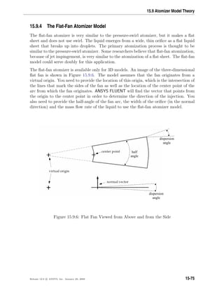
![Discrete Phase
The breakup of the flat fan is calculated very much like the breakup of the sheet in the
pressure-swirl atomizer. The sheet breaks up into ligaments which then form individual
droplets. The only difference is that for short waves, the flat fan sheet is assumed to form
ligaments at half-wavelength intervals. Hence the ligament diameter for short waves is
given by
dL =
16h
Ks
(15.9-36)
In this case, dL in Equation 15.9-36 is taken to be the most probable diameter, with a
Rosin-Rammler spread parameter of 3.5 and a default dispersion angle of 6◦
. This angle
can be set in the Set Injection Properties dialog box. In all other respects, the flat-fan
atomizer model is like the sheet breakup portion of the pressure-swirl atomizer.
15.9.5 The Effervescent Atomizer Model
Effervescent atomization is the injection of liquid infused with a super-heated (with
respect to downstream conditions) liquid or propellant. As the volatile liquid exits the
nozzle, it rapidly changes phase. This phase change quickly breaks up the stream into
small droplets with a wide dispersion angle. The model also applies to cases where a
very hot liquid is discharged.
Since the physics of effervescence is not well understood, the model must rely on rough
empirical fits. The photographs of Reitz and Bracco [288] provide some insights. These
photographs show a dense liquid core to the spray, surrounded by a wide shroud of smaller
droplets.
The initial velocity of the droplets is computed from conservation of mass, assuming the
exiting jet has a cross-sectional area that is Cct times the nozzle area, where Cct is a fixed
constant, equal to 0.611 as specified in Equations 15.9-3 and 15.9-12.
u =
˙meff
ρlCctA
(15.9-37)
The maximum droplet diameter is set to the effective diameter of the exiting jet:
dmax = d Cct (15.9-38)
15-76 Release 12.0 c ANSYS, Inc. January 29, 2009](https://image.slidesharecdn.com/flth-130501182911-phpapp02/85/Flth-508-320.jpg)

![Discrete Phase
15.10.1 Taylor Analogy Breakup (TAB) Model
Introduction
The Taylor analogy breakup (TAB) model is a classic method for calculating droplet
breakup, which is applicable to many engineering sprays. This method is based upon
Taylor’s analogy [347] between an oscillating and distorting droplet and a spring mass
system. Table 15.10.1 illustrates the analogous components.
Table 15.10.1: Comparison of a Spring-Mass System to a Distorting Droplet
Spring-Mass System Distorting and Oscillating Droplet
restoring force of spring surface tension forces
external force droplet drag force
damping force droplet viscosity forces
The resulting TAB model equation set, which governs the oscillating and distorting
droplet, can be solved to determine the droplet oscillation and distortion at any given
time. As described in detail below, when the droplet oscillations grow to a critical value
the “parent” droplet will break up into a number of smaller “child” droplets. As a
droplet is distorted from a spherical shape, the drag coefficient changes. A drag model
that incorporates the distorting droplet effects is available in ANSYS FLUENT. See Sec-
tion 15.3.5: Dynamic Drag Model Theory for details.
Use and Limitations
The TAB model is best for low-Weber-number sprays. Extremely high-Weber-number
sprays result in shattering of droplets, which is not described well by the spring-mass
analogy.
Droplet Distortion
The equation governing a damped, forced oscillator is [256]
F − kx − d
dx
dt
= m
d2
x
dt2
(15.10-1)
where x is the displacement of the droplet equator from its spherical (undisturbed) po-
sition. The coefficients of this equation are taken from Taylor’s analogy:
F
m
= CF
ρgu2
ρlr
(15.10-2)
15-78 Release 12.0 c ANSYS, Inc. January 29, 2009](https://image.slidesharecdn.com/flth-130501182911-phpapp02/85/Flth-510-320.jpg)
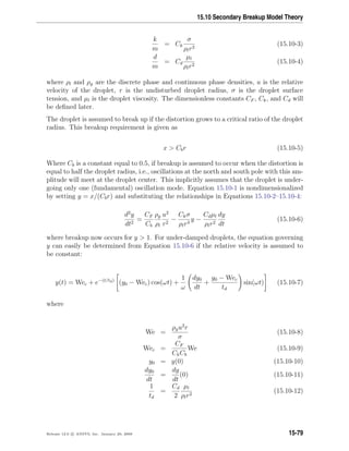
![Discrete Phase
ω2
= Ck
σ
ρlr3
−
1
t2
d
(15.10-13)
In Equation 15.10-7, u is the relative velocity between the droplet and the gas phase
and We is the droplet Weber number, a dimensionless parameter defined as the ratio
of aerodynamic forces to surface tension forces. The droplet oscillation frequency is
represented by ω. The default value of y0 is 0, based upon the work of Liu et al. [205].
The constants have been chosen to match experiments and theory [174]:
Ck = 8
Cd = 5
CF =
1
3
If Equation 15.10-7 is solved for all droplets, those with y 1 are assumed to break up.
The size and velocity of the new child droplets must be determined.
Size of Child Droplets
The size of the child droplets is determined by equating the energy of the parent droplet
to the combined energy of the child droplets. The energy of the parent droplet is [256]
Eparent = 4πr2
σ + K
π
5
ρlr5
dy
dt
2
+ ω2
y2
(15.10-14)
where K is the ratio of the total energy in distortion and oscillation to the energy in the
fundamental mode, of the order (10
3
). The child droplets are assumed to be nondistorted
and nonoscillating. Thus, the energy of the child droplets can be shown to be
Echild = 4πr2
σ
r
r32
+
π
6
ρlr5 dy
dt
2
(15.10-15)
where r32 is the Sauter mean radius of the droplet size distribution. r32 can be found
by equating the energy of the parent and child droplets (i.e., Equations 15.10-14 and
15.10-15), setting y = 1, and ω2
= 8σ/ρlr3
:
r32 =
r
1 + 8Ky2
20
+ ρlr3(dy/dt)2
σ
6K−5
120
(15.10-16)
Once the size of the child droplets is determined, the number of child droplets can easily
be determined by mass conservation.
15-80 Release 12.0 c ANSYS, Inc. January 29, 2009](https://image.slidesharecdn.com/flth-130501182911-phpapp02/85/Flth-512-320.jpg)
![15.10 Secondary Breakup Model Theory
Velocity of Child Droplets
The TAB model allows for a velocity component normal to the parent droplet velocity
to be imposed upon the child droplets. When breakup occurs, the equator of the parent
droplet is traveling at a velocity of dx/dt = Cbr(dy/dt). Therefore, the child droplets
will have a velocity normal to the parent droplet velocity given by
vnormal = CvCbr
dy
dt
(15.10-17)
where Cv is a constant of order (1).
Droplet Breakup
To model droplet breakup, the TAB model first determines the amplitude for an un-
damped oscillation (td ≈ ∞) for each droplet at time step n using the following:
A = (yn − Wec)2 +
(dy/dt)n
ω
2
(15.10-18)
According to Equation 15.10-18, breakup is possible only if the following condition is
satisfied:
Wec + A 1 (15.10-19)
This is the limiting case, as damping will only reduce the chance of breakup. If a
droplet fails the above criterion, breakup does not occur. The only additional calculations
required then, are to update y using a discretized form of Equation 15.10-7 and its
derivative, which are both based on work done by O’Rourke and Amsden [256]:
yn+1
= Wec + e−(∆t/td)
(yn
− Wec) cos(ωt) +
1
ω
dy
dt
n
+
yn
− Wec
td
sin(ωt)
(15.10-20)
dy
dt
n+1
=
Wec − yn+1
td
+
ωe−(∆t/td) 1
ω
dy
dt
n
+
yn
− Wec
td
cos(ω∆t) − (yn
− Wec) sin(ω∆t) (15.10-21)
Release 12.0 c ANSYS, Inc. January 29, 2009 15-81](https://image.slidesharecdn.com/flth-130501182911-phpapp02/85/Flth-513-320.jpg)
![Discrete Phase
All of the constants in these expressions are assumed to be constant throughout the time
step.
If the criterion of Equation 15.10-19 is met, then breakup is possible. The breakup
time, tbu, must be determined to see if breakup occurs within the time step ∆t. The
value of tbu is set to the time required for oscillations to grow sufficiently large that the
magnitude of the droplet distortion, y, is equal to unity. The breakup time is determined
under the assumption that the droplet oscillation is undamped for its first period. The
breakup time is therefore the smallest root greater than tn
of an undamped version of
Equation 15.10-7:
Wec + A cos[ω(t − tn
) + φ] = 1 (15.10-22)
where
cos φ =
yn
− Wec
A
(15.10-23)
and
sin φ = −
(dy/dt)n
Aω
(15.10-24)
If tbu tn+1
, then breakup will not occur during the current time step, and y and
(dy/dt) are updated by Equations 15.10-20 and 15.10-21. The breakup calculation then
continues with the next droplet. Conversely, if tn
tbu tn+1
, then breakup will occur
and the child droplet radii are determined by Equation 15.10-16. The number of child
droplets, N, is determined by mass conservation:
Nn+1
= Nn rn
rn+1
3
(15.10-25)
It is assumed that the child droplets are neither distorted nor oscillating; i.e., y =
(dy/dt) = 0. The child droplets are represented by a number of child parcels which
are created from the original parcel. These child parcels are distributed equally along
the equator of the parent droplet in a plane normal to the parent relative velocity vector.
The diameter of each of the child parcels is sampled from a Rosin Rammler distribution
based on the Sauter mean radius (Equation 15.10-16) and a spread parameter of 3.5.
15-82 Release 12.0 c ANSYS, Inc. January 29, 2009](https://image.slidesharecdn.com/flth-130501182911-phpapp02/85/Flth-514-320.jpg)
![15.10 Secondary Breakup Model Theory
A velocity component normal to the relative velocity vector, with magnitude computed
by Equation 15.10-17, is imposed upon the child droplets. It is decomposed at the equator
into components pointing radially outward.
i A large number of child parcels ensures a smooth distribution of particle
diameters and source terms which is needed when simulating, for example,
evaporating sprays.
15.10.2 Wave Breakup Model
Introduction
An alternative to the TAB model that is appropriate for high-Weber-number flows is the
wave breakup model of Reitz [287], which considers the breakup of the droplets to be
induced by the relative velocity between the gas and liquid phases. The model assumes
that the time of breakup and the resulting droplet size are related to the fastest-growing
Kelvin-Helmholtz instability, derived from the jet stability analysis described below. The
wavelength and growth rate of this instability are used to predict details of the newly-
formed droplets.
Use and Limitations
The wave model is appropriate for high-speed injections, where the Kelvin-Helmholtz
instability is believed to dominate droplet breakup (We 100). Because this breakup
model can increase the number of computational parcels, you may wish to inject a modest
number of droplets initially.
Jet Stability Analysis
The jet stability analysis described in detail by Reitz and Bracco [289] is presented briefly
here. The analysis considers the stability of a cylindrical, viscous, liquid jet of radius
a issuing from a circular orifice at a velocity v into a stagnant, incompressible, inviscid
gas of density ρ2. The liquid has a density, ρ1, and viscosity, µ1, and a cylindrical
polar coordinate system is used which moves with the jet. An arbitrary infinitesimal
axisymmetric surface displacement of the form
η = η0eikz+ωt
(15.10-26)
is imposed on the initially steady motion and it is thus desired to find the dispersion
relation ω = ω(k) which relates the real part of the growth rate, ω, to its wave number,
k = 2π/λ.
Release 12.0 c ANSYS, Inc. January 29, 2009 15-83](https://image.slidesharecdn.com/flth-130501182911-phpapp02/85/Flth-515-320.jpg)
![Discrete Phase
In order to determine the dispersion relation, the linearized equations for the hydrody-
namics of the liquid are solved assuming wave solutions of the form
φ1 = C1I0(kr)eikz+ωt
(15.10-27)
ψ1 = C2I1(Lr)eikz+ωt
(15.10-28)
where φ1 and ψ1 are the velocity potential and stream function, respectively, C1 and
C2 are integration constants, I0 and I1 are modified Bessel functions of the first kind,
L2
= k2
+ ω/ν1, and ν1 is the liquid kinematic viscosity [287]. The liquid pressure is
obtained from the inviscid part of the liquid equations. In addition, the inviscid gas
equations can be solved to obtain the fluctuating gas pressure at r = a:
− p21 = −ρ2(U − iωk)2
kη
K0(ka)
K1(ka)
(15.10-29)
where K0 and K1 are modified Bessel functions of the second kind and u is the relative
velocity between the liquid and the gas. The linearized boundary conditions are
v1 =
∂η
∂t
(15.10-30)
∂u1
∂r
= −
∂v1
∂z
(15.10-31)
and
− p1 + 2µ1 −
σ
a2
η + a2 ∂2
η
∂z2
+ p2 = 0 (15.10-32)
which are mathematical statements of the liquid kinematic free surface condition, conti-
nuity of shear stress, and continuity of normal stress, respectively. Note that u1 is the
axial perturbation liquid velocity, v1 is the radial perturbation liquid velocity, and σ is
the surface tension. Also note that Equation 15.10-31 was obtained under the assumption
that v2 = 0.
15-84 Release 12.0 c ANSYS, Inc. January 29, 2009](https://image.slidesharecdn.com/flth-130501182911-phpapp02/85/Flth-516-320.jpg)
![15.10 Secondary Breakup Model Theory
As described by Reitz [287], Equations 15.10-30 and 15.10-31 can be used to eliminate
the integration constants C1 and C2 in Equations 15.10-27 and 15.10-28. Thus, when
the pressure and velocity solutions are substituted into Equation 15.10-32, the desired
dispersion relation is obtained:
ω2
+ 2ν1k2
ω
I1(ka)
I0(ka)
−
2kL
k2 + L2
I1(ka)
I0(ka)
I1(La)
I1(La)
=
σk
ρ1a2
(1−k2
a2
)
L2
− a2
L2 + a2
I1(ka)
I0(ka)
+
ρ2
ρ1
U − i
ω
k
2 L2
− a2
L2 + a2
I1(ka)
I0(ka)
K0(ka)
K1(ka)
(15.10-33)
As shown by Reitz [287], Equation 15.10-33 predicts that a maximum growth rate (or
most unstable wave) exists for a given set of flow conditions. Curve fits of numerical
solutions to Equation 15.10-33 were generated for the maximum growth rate, Ω, and the
corresponding wavelength, Λ, and are given by Reitz [287]:
Λ
a
= 9.02
(1 + 0.45Oh0.5
)(1 + 0.4Ta0.7
)
(1 + 0.87We1.67
2 )0.6
(15.10-34)
Ω
ρ1a3
σ
=
(0.34 + 0.38We1.5
2 )
(1 + Oh)(1 + 1.4Ta0.6
)
(15.10-35)
where Oh =
√
We1/Re1 is the Ohnesorge number and Ta = Oh
√
We2 is the Taylor
number. Furthermore, We1 = ρ1U2
a/σ and We2 = ρ2U2
a/σ are the liquid and gas
Weber numbers, respectively, and Re1 = Ua/ν1 is the Reynolds number.
Droplet Breakup
In the wave model, breakup of droplet parcels is calculated by assuming that the radius
of the newly-formed droplets is proportional to the wavelength of the fastest-growing
unstable surface wave on the parent droplet. In other words,
r = B0Λ (15.10-36)
where B0 is a model constant set equal to 0.61 based on the work of Reitz [287]. Fur-
thermore, the rate of change of droplet radius in the parent parcel is given by
da
dt
= −
(a − r)
τ
, r ≤ a (15.10-37)
Release 12.0 c ANSYS, Inc. January 29, 2009 15-85](https://image.slidesharecdn.com/flth-130501182911-phpapp02/85/Flth-517-320.jpg)
![Discrete Phase
where the breakup time, τ, is given by
τ =
3.726B1a
ΛΩ
(15.10-38)
and Λ and Ω are obtained from Equations 15.10-34 and 15.10-35, respectively. The
breakup time constant, B1, is set to a value of 1.73 as recommended by Liu et al. [205].
Values of B1 can range between 1 and 60, depending on the injector characterization.
In the wave model, mass is accumulated from the parent drop at a rate given by Equa-
tion 15.10-38 until the shed mass is equal to 5% of the initial parcel mass. At this time, a
new parcel is created with a radius given by Equation 15.10-36. The new parcel is given
the same properties as the parent parcel (i.e., temperature, material, position, etc.) with
the exception of radius and velocity. The new parcel is given a component of velocity
randomly selected in the plane orthogonal to the direction vector of the parent parcel,
and the momentum of the parent parcel is adjusted so that momentum is conserved. The
velocity magnitude of the new parcel is the same as the parent parcel.
You must also specify the model constants which determine how the gas phase interacts
with the liquid droplets. For example, the breakup time constant B1 is the constant
multiplying the time scale which determines how quickly the parcel will loose mass.
Therefore, a larger number means that it takes longer for the particle to loose a given
amount. A larger number for B1 in the context of interaction with the gas phase would
mean that the interaction with the subgrid is less intense. B0 is the constant for the drop
size and is generally taken to be 0.61.
15.11 Droplet Collision and Coalescence Model Theory
15.11.1 Introduction
When your simulation includes tracking of droplets, ANSYS FLUENT provides an option
for estimating the number of droplet collisions and their outcomes in a computationally
efficient manner. The difficulty in any collision calculation is that for N droplets, each
droplet has N −1 possible collision partners. Thus, the number of possible collision pairs
is approximately 1
2
N2
. (The factor of 1
2
appears because droplet A colliding with droplet
B is identical to droplet B colliding with droplet A. This symmetry reduces the number
of possible collision events by half.)
An important consideration is that the collision algorithm must calculate 1
2
N2
possible
collision events at every time step. Since a spray can consist of several million droplets,
the computational cost of a collision calculation from first principles is prohibitive. This
motivates the concept of parcels. Parcels are statistical representations of a number of
individual droplets. For example, if ANSYS FLUENT tracks a set of parcels, each of which
represents 1000 droplets, the cost of the collision calculation is reduced by a factor of
106
. Because the cost of the collision calculation still scales with the square of N, the
15-86 Release 12.0 c ANSYS, Inc. January 29, 2009](https://image.slidesharecdn.com/flth-130501182911-phpapp02/85/Flth-518-320.jpg)
![15.11 Droplet Collision and Coalescence Model Theory
reduction of cost is significant; however, the effort to calculate the possible intersection
of so many parcel trajectories would still be prohibitively expensive.
The algorithm of O’Rourke [255] efficiently reduces the computational cost of the spray
calculation. Rather than using geometry to see if parcel paths intersect, O’Rourke’s
method is a stochastic estimate of collisions. O’Rourke also makes the assumption that
two parcels may collide only if they are located in the same continuous-phase cell. These
two assumptions are valid only when the continuous-phase cell size is small compared
to the size of the spray. For these conditions, the method of O’Rourke is second-order
accurate at estimating the chance of collisions. The concept of parcels together with
the algorithm of O’Rourke makes the calculation of collision possible for practical spray
problems.
Once it is decided that two parcels of droplets collide, the algorithm further determines
the type of collision. Only coalescence and bouncing outcomes are considered. The
probability of each outcome is calculated from the collisional Weber number (Wec) and
a fit to experimental observations. Here,
Wec =
ρU2
relD
σ
(15.11-1)
where Urel is the relative velocity between two parcels and D is the arithmetic mean
diameter of the two parcels. The state of the two colliding parcels is modified based on
the outcome of the collision.
15.11.2 Use and Limitations
The collision model assumes that the frequency of collisions is much less than the par-
ticle time step. If the particle time step is too large, then the results may be time-
step-dependent. You should adjust the particle length scale accordingly. Additionally,
the model is most applicable for low-Weber-number collisions where collisions result in
bouncing and coalescence. Above a Weber number of about 100, the outcome of collision
could be shattering.
Sometimes the collision model can cause mesh-dependent artifacts to appear in the spray.
This is a result of the assumption that droplets can collide only within the same cell.
These tend to be visible when the source of injection is at a mesh vertex. The coalescence
of droplets tends to cause the spray to pull away from cell boundaries. In two dimensions,
a finer mesh and more computational droplets can be used to reduce these effects. In
three dimensions, best results are achieved when the spray is modeled using a polar mesh
with the spray at the center.
If the collision model is used in a transient simulation, multiple DPM iterations per time
step cannot be specified in the Number of Continuous Phase Iterations per DPM Iteration
field in the Discrete Phase Model dialog box. In such cases, only one DPM iteration
per time step will be calculated.
Release 12.0 c ANSYS, Inc. January 29, 2009 15-87](https://image.slidesharecdn.com/flth-130501182911-phpapp02/85/Flth-519-320.jpg)
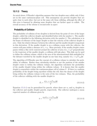
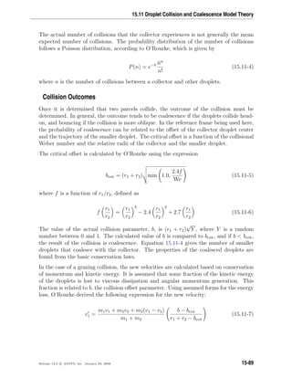
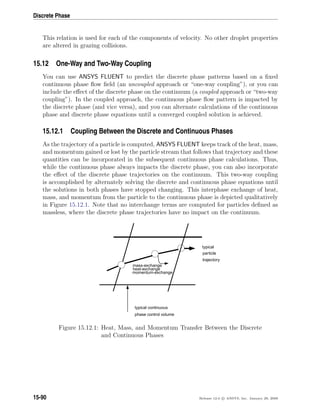
![15.12 One-Way and Two-Way Coupling
15.12.2 Momentum Exchange
The momentum transfer from the continuous phase to the discrete phase is computed in
ANSYS FLUENT by examining the change in momentum of a particle as it passes through
each control volume in the ANSYS FLUENT model. This momentum change is computed
as
F =
18µCDRe
ρpd2
p24
(up − u) + Fother ˙mp∆t (15.12-1)
where
µ = viscosity of the fluid
ρp = density of the particle
dp = diameter of the particle
Re = relative Reynolds number
up = velocity of the particle
u = velocity of the fluid
CD = drag coefficient
˙mp = mass flow rate of the particles
∆t = time step
Fother = other interaction forces
This momentum exchange appears as a momentum source in the continuous phase mo-
mentum balance in any subsequent calculations of the continuous phase flow field and
can be reported by ANSYS FLUENT as described in Section 23.7: Postprocessing for the
Discrete Phase in the separate User’s Guide.
15.12.3 Heat Exchange
The heat transfer from the continuous phase to the discrete phase is computed in ANSYS
FLUENT by examining the change in thermal energy of a particle as it passes through
each control volume in the ANSYS FLUENT model. In the absence of a chemical reaction
(i.e., for all particle laws except Law 5) the heat exchange is computed as
Q =
˙mp,0
mp,0
(mpin − mpout)[−Hlatref + Hpyrol] − mpout
Tpout
Tref
cppdT + mpin
Tpin
Tref
cppdT
(15.12-2)
Release 12.0 c ANSYS, Inc. January 29, 2009 15-91](https://image.slidesharecdn.com/flth-130501182911-phpapp02/85/Flth-523-320.jpg)
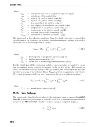
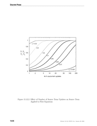

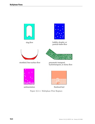
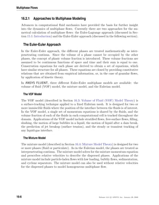
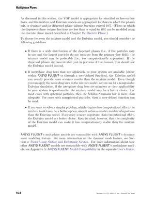
![16.2 Choosing a General Multiphase Model
Detailed Guidelines
For stratified and slug flows, the choice of the VOF model, as indicated in Section 16.2.2: Model
Comparisons, is straightforward. Choosing a model for the other types of flows is less
straightforward. As a general guide, there are some parameters that help to identify the
appropriate multiphase model for these other flows: the particulate loading, β, and the
Stokes number, St. (Note that the word “particle” is used in this discussion to refer to
a particle, droplet, or bubble.)
The Effect of Particulate Loading
Particulate loading has a major impact on phase interactions. The particulate loading is
defined as the mass density ratio of the dispersed phase (d) to that of the carrier phase
(c):
β =
αdρd
αcρc
(16.2-1)
The material density ratio
γ =
ρd
ρc
(16.2-2)
is greater than 1000 for gas-solid flows, about 1 for liquid-solid flows, and less than 0.001
for gas-liquid flows.
Using these parameters it is possible to estimate the average distance between the indi-
vidual particles of the particulate phase. An estimate of this distance has been given by
Crowe et al. [62]:
L
dd
=
π
6
1 + κ
κ
1/3
(16.2-3)
where κ = β
γ
. Information about these parameters is important for determining how the
dispersed phase should be treated. For example, for a gas-particle flow with a particulate
loading of 1, the interparticle space L
dd
is about 8; the particle can therefore be treated
as isolated (i.e., very low particulate loading).
Release 12.0 c ANSYS, Inc. January 29, 2009 16-9](https://image.slidesharecdn.com/flth-130501182911-phpapp02/85/Flth-537-320.jpg)
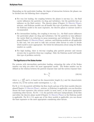
![Multiphase Flows
As a fully implicit scheme, this second-order time-accurate scheme achieves its accuracy
by using an Euler backward approximation in time (see Equation 18.3-17). The general
transport equation, Equation 16.2-5 is discretized as
3(αpρpφpV ol)n+1
− 4(αpρpφpV ol)n
+ (αpρpφp)n−1
2∆t
= (16.2-6)
[Anb(φnb − φp)]n+1
+ SU
n+1
− Sp
n+1
φp
n+1
Equation 16.2-6 can be written in simpler form:
Apφp = Anbφnb + Sφ (16.2-7)
where
Ap = Anb
n+1
+ Sp
n+1
+ 1.5(αpρpV ol)n+1
∆t
Sφ = SU
n+1
+ 2(αpρpφpV ol)n−0.5(αpρpφpV ol)n−1
∆t
This scheme is easily implemented based on ANSYS FLUENT’s existing first-order Euler
scheme. It is unconditionally stable, however, the negative coefficient at the time level
tn−1, of the three-time level method, may produce oscillatory solutions if the time steps
are large.
This problem can be eliminated if a bounded second-order scheme is introduced. How-
ever, oscillating solutions are most likely seen in compressible liquid flows. Therefore, in
this version of ANSYS FLUENT, a bounded second-order time scheme has been imple-
mented for compressible liquid flows only. For single phase and multiphase compressible
liquid flows, the second-order time scheme is, by default, the bounded scheme.
16.2.4 Stability and Convergence
The process of solving a multiphase system is inherently difficult and you may encounter
some stability or convergence problems.
When solving a time-dependent problem, a proper initial field is required to avoid in-
stabilities, which usually arise from poor initial fields. If the CPU time is a concern for
transient problems, then the best option is to use PC SIMPLE. When body forces are
significant, or if the solution requires higher order numerical schemes, it is recommended
that you start with a small time step, which can be increased after performing a few time
steps to get a better approximation of the pressure field.
For a steady solution, it is recommended that you use the Multiphase Coupled solver, de-
scribed in detail in Section 24.7.1: Coupled Solution for Multiphase Flows in the separate
User’s Guide. The iterative nature of this solver requires a good starting patched field.
16-12 Release 12.0 c ANSYS, Inc. January 29, 2009](https://image.slidesharecdn.com/flth-130501182911-phpapp02/85/Flth-540-320.jpg)
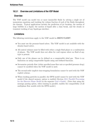
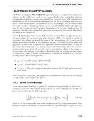
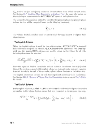
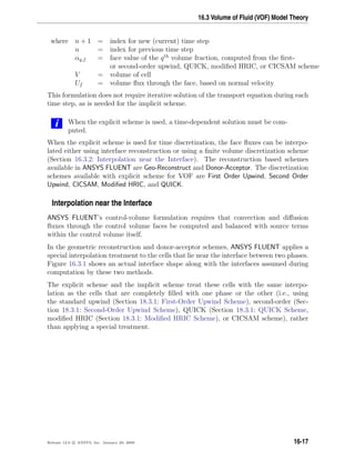
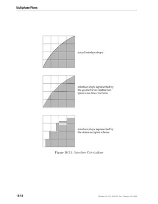
![16.3 Volume of Fluid (VOF) Model Theory
The Geometric Reconstruction Scheme
In the geometric reconstruction approach, the standard interpolation schemes that are
used in ANSYS FLUENT are used to obtain the face fluxes whenever a cell is completely
filled with one phase or another. When the cell is near the interface between two phases,
the geometric reconstruction scheme is used.
The geometric reconstruction scheme represents the interface between fluids using a
piecewise-linear approach. In ANSYS FLUENT this scheme is the most accurate and
is applicable for general unstructured meshes. The geometric reconstruction scheme is
generalized for unstructured meshes from the work of Youngs [388]. It assumes that the
interface between two fluids has a linear slope within each cell, and uses this linear shape
for calculation of the advection of fluid through the cell faces. (See Figure 16.3.1.)
The first step in this reconstruction scheme is calculating the position of the linear in-
terface relative to the center of each partially-filled cell, based on information about
the volume fraction and its derivatives in the cell. The second step is calculating the
advecting amount of fluid through each face using the computed linear interface repre-
sentation and information about the normal and tangential velocity distribution on the
face. The third step is calculating the volume fraction in each cell using the balance of
fluxes calculated during the previous step.
i When the geometric reconstruction scheme is used, a time-dependent solu-
tion must be computed. Also, if you are using a conformal mesh (i.e., if the
mesh node locations are identical at the boundaries where two subdomains
meet), you must ensure that there are no two-sided (zero-thickness) walls
within the domain. If there are, you will need to slit them, as described in
Section 6.8.6: Slitting Face Zones in the separate User’s Guide.
The Donor-Acceptor Scheme
In the donor-acceptor approach, the standard interpolation schemes that are used in
ANSYS FLUENT are used to obtain the face fluxes whenever a cell is completely filled
with one phase or another. When the cell is near the interface between two phases, a
“donor-acceptor” scheme is used to determine the amount of fluid advected through the
face [131]. This scheme identifies one cell as a donor of an amount of fluid from one phase
and another (neighbor) cell as the acceptor of that same amount of fluid, and is used to
prevent numerical diffusion at the interface. The amount of fluid from one phase that
can be convected across a cell boundary is limited by the minimum of two values: the
filled volume in the donor cell or the free volume in the acceptor cell.
Release 12.0 c ANSYS, Inc. January 29, 2009 16-19](https://image.slidesharecdn.com/flth-130501182911-phpapp02/85/Flth-547-320.jpg)
![Multiphase Flows
The orientation of the interface is also used in determining the face fluxes. The interface
orientation is either horizontal or vertical, depending on the direction of the volume
fraction gradient of the qth
phase within the cell, and that of the neighbor cell that shares
the face in question. Depending on the interface’s orientation as well as its motion, flux
values are obtained by pure upwinding, pure downwinding, or some combination of the
two.
i When the donor-acceptor scheme is used, a time-dependent solution must
be computed. Also, the donor-acceptor scheme can be used only with
quadrilateral or hexahedral meshes. In addition, if you are using a confor-
mal mesh (i.e., if the mesh node locations are identical at the boundaries
where two subdomains meet), you must ensure that there are no two-sided
(zero-thickness) walls within the domain. If there are, you will need to
slit them, as described in Section 6.8.6: Slitting Face Zones in the separate
User’s Guide.
The Compressive Interface Capturing Scheme for Arbitrary Meshes (CICSAM)
The compressive interface capturing scheme for arbitrary meshes (CICSAM), based on
Ubbink’s work [351], is a high resolution differencing scheme. The CICSAM scheme is
particularly suitable for flows with high ratios of viscosities between the phases. CICSAM
is implemented in ANSYS FLUENT as an explicit scheme and offers the advantage of
producing an interface that is almost as sharp as the geometric reconstruction scheme.
16.3.3 Material Properties
The properties appearing in the transport equations are determined by the presence of
the component phases in each control volume. In a two-phase system, for example, if
the phases are represented by the subscripts 1 and 2, and if the volume fraction of the
second of these is being tracked, the density in each cell is given by
ρ = α2ρ2 + (1 − α2)ρ1 (16.3-5)
In general, for an n-phase system, the volume-fraction-averaged density takes on the
following form:
ρ = αqρq (16.3-6)
All other properties (e.g., viscosity) are computed in this manner.
16-20 Release 12.0 c ANSYS, Inc. January 29, 2009](https://image.slidesharecdn.com/flth-130501182911-phpapp02/85/Flth-548-320.jpg)
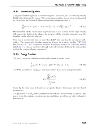
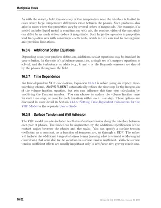
![16.3 Volume of Fluid (VOF) Model Theory
Surface Tension
Surface tension arises as a result of attractive forces between molecules in a fluid. Con-
sider an air bubble in water, for example. Within the bubble, the net force on a molecule
due to its neighbors is zero. At the surface, however, the net force is radially inward, and
the combined effect of the radial components of force across the entire spherical surface
is to make the surface contract, thereby increasing the pressure on the concave side of
the surface. The surface tension is a force, acting only at the surface, that is required
to maintain equilibrium in such instances. It acts to balance the radially inward inter-
molecular attractive force with the radially outward pressure gradient force across the
surface. In regions where two fluids are separated, but one of them is not in the form
of spherical bubbles, the surface tension acts to minimize free energy by decreasing the
area of the interface.
The surface tension model in ANSYS FLUENT is the continuum surface force (CSF) model
proposed by Brackbill et al. [34]. With this model, the addition of surface tension to the
VOF calculation results in a source term in the momentum equation. To understand the
origin of the source term, consider the special case where the surface tension is constant
along the surface, and where only the forces normal to the interface are considered. It
can be shown that the pressure drop across the surface depends upon the surface tension
coefficient, σ, and the surface curvature as measured by two radii in orthogonal directions,
R1 and R2:
p2 − p1 = σ
1
R1
+
1
R2
(16.3-10)
where p1 and p2 are the pressures in the two fluids on either side of the interface.
In ANSYS FLUENT, a formulation of the CSF model is used, where the surface curvature
is computed from local gradients in the surface normal at the interface. Let n be the
surface normal, defined as the gradient of αq, the volume fraction of the qth
phase.
n = αq (16.3-11)
The curvature, κ, is defined in terms of the divergence of the unit normal, ˆn [34]:
κ = · ˆn (16.3-12)
where
ˆn =
n
|n|
(16.3-13)
Release 12.0 c ANSYS, Inc. January 29, 2009 16-23](https://image.slidesharecdn.com/flth-130501182911-phpapp02/85/Flth-551-320.jpg)
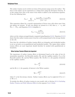
![16.3 Volume of Fluid (VOF) Model Theory
Wall Adhesion
An option to specify a wall adhesion angle in conjunction with the surface tension model
is also available in the VOF model. The model is taken from work done by Brackbill et
al. [34]. Rather than impose this boundary condition at the wall itself, the contact angle
that the fluid is assumed to make with the wall is used to adjust the surface normal in
cells near the wall. This so-called dynamic boundary condition results in the adjustment
of the curvature of the surface near the wall.
If θw is the contact angle at the wall, then the surface normal at the live cell next to the
wall is
ˆn = ˆnw cos θw + ˆtw sin θw (16.3-18)
where ˆnw and ˆtw are the unit vectors normal and tangential to the wall, respectively.
The combination of this contact angle with the normally calculated surface normal one
cell away from the wall determine the local curvature of the surface, and this curvature
is used to adjust the body force term in the surface tension calculation.
To include wall adhesion in your model, refer to Section 24.3.4: Including Surface Tension
and Wall Adhesion Effects in the separate User’s Guide.
16.3.9 Open Channel Flow
ANSYS FLUENT can model the effects of open channel flow (e.g., rivers, dams, and
surface-piercing structures in unbounded stream) using the VOF formulation and the
open channel boundary condition. These flows involve the existence of a free surface
between the flowing fluid and fluid above it (generally the atmosphere). In such cases,
the wave propagation and free surface behavior becomes important. Flow is generally
governed by the forces of gravity and inertia. This feature is mostly applicable to marine
applications and the analysis of flows through drainage systems.
Open channel flows are characterized by the dimensionless Froude Number, which is
defined as the ratio of inertia force and hydrostatic force.
Fr =
V
√
gy
(16.3-19)
where V is the velocity magnitude, g is gravity, and y is a length scale, in this case,
the distance from the bottom of the channel to the free surface. The denominator in
Equation 16.3-19 is the propagation speed of the wave. The wave speed as seen by the
fixed observer is defined as
Vw = V ±
√
gy (16.3-20)
Release 12.0 c ANSYS, Inc. January 29, 2009 16-25](https://image.slidesharecdn.com/flth-130501182911-phpapp02/85/Flth-553-320.jpg)
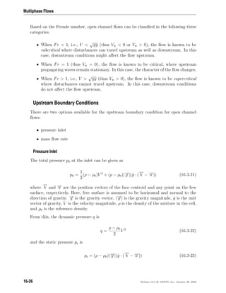
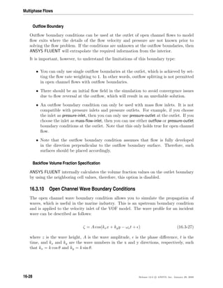
![16.3 Volume of Fluid (VOF) Model Theory
The wave number k is defined as
k =
2π
λ
(16.3-28)
where λ is the wave length and the effective wave frequency ωe is
ωe = ω + kU (16.3-29)
U is the uniform incident wave velocity and ω, the wave frequency, is defined as
ω = gk tanh(kh) (16.3-30)
where h is the liquid height and g is the gravity magnitude.
The velocity components for the incident wave boundary condition can be described in
terms of shallow waves and short gravity waves.
Shallow waves are defined as
u
v
=
gkA
ω
cosh[k(z + h)]
cosh(kh)
cos θ
sin θ
cos(kxx + kyy − ωet + ) (16.3-31)
w =
gkA
ω
sinh[k(z + h)]
cosh(kh)
sin(kxx + kyy − ωet + ) (16.3-32)
Short gravity waves are defined as
u
v
=
gkA
ω
ekz cos θ
sin θ
cos(kxx + kyy − ωet + ) (16.3-33)
w =
gkA
ω
ekz
sin(kxx + kyy − ωet + ) (16.3-34)
where u, v, and w are the velocity components. Note that direction specifications for
the velocity components are such that u is based on the flow direction specified in the
wave velocity specification method, w is based on the gravity direction, and v is in the
cross direction of the flow and gravity direction. For more information on how to use
and set up this model, refer to Section 24.3.2: Modeling Open Channel Wave Boundary
Conditions in the separate User’s Guide.
Release 12.0 c ANSYS, Inc. January 29, 2009 16-29](https://image.slidesharecdn.com/flth-130501182911-phpapp02/85/Flth-557-320.jpg)
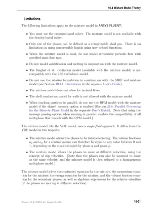
![16.4 Mixture Model Theory
16.4.4 Energy Equation
The energy equation for the mixture takes the following form:
∂
∂t
n
k=1
(αkρkEk) + ·
n
k=1
(αkvk(ρkEk + p)) = · (keff T) + SE (16.4-7)
where keff is the effective conductivity ( αk(kk + kt)), where kt is the turbulent thermal
conductivity, defined according to the turbulence model being used). The first term on
the right-hand side of Equation 16.4-7 represents energy transfer due to conduction. SE
includes any other volumetric heat sources.
In Equation 16.4-7,
Ek = hk −
p
ρk
+
v2
k
2
(16.4-8)
for a compressible phase, and Ek = hk for an incompressible phase, where hk is the
sensible enthalpy for phase k.
16.4.5 Relative (Slip) Velocity and the Drift Velocity
The relative velocity (also referred to as the slip velocity) is defined as the velocity of a
secondary phase (p) relative to the velocity of the primary phase (q):
vpq = vp − vq (16.4-9)
The mass fraction for any phase (k) is defined as
ck =
αkρk
ρm
(16.4-10)
The drift velocity and the relative velocity (vqp) are connected by the following expression:
vdr,p = vpq −
n
k=1
ckvqk (16.4-11)
ANSYS FLUENT’s mixture model makes use of an algebraic slip formulation. The basic
assumption of the algebraic slip mixture model is that to prescribe an algebraic relation
for the relative velocity, a local equilibrium between the phases should be reached over
a short spatial length scale. Following Manninen et al. [217], the form of the relative
velocity is given by:
Release 12.0 c ANSYS, Inc. January 29, 2009 16-33](https://image.slidesharecdn.com/flth-130501182911-phpapp02/85/Flth-561-320.jpg)
![Multiphase Flows
vpq =
τp
fdrag
(ρp − ρm)
ρp
a (16.4-12)
where τp is the particle relaxation time
τp =
ρpd2
p
18µq
(16.4-13)
d is the diameter of the particles (or droplets or bubbles) of secondary phase p, a is the
secondary-phase particle’s acceleration. The default drag function fdrag is taken from
Schiller and Naumann [305]:
fdrag =
1 + 0.15 Re0.687
Re ≤ 1000
0.0183 Re Re 1000
(16.4-14)
and the acceleration a is of the form
a = g − (vm · )vm −
∂vm
∂t
(16.4-15)
The simplest algebraic slip formulation is the so-called drift flux model, in which the ac-
celeration of the particle is given by gravity and/or a centrifugal force and the particulate
relaxation time is modified to take into account the presence of other particles.
In turbulent flows the relative velocity should contain a diffusion term due to the dis-
persion appearing in the momentum equation for the dispersed phase. ANSYS FLUENT
adds this dispersion to the relative velocity:
vpq =
(ρp − ρm)d2
p
18µqfdrag
a −
ηt
σt
αp
αp
−
αq
αq
(16.4-16)
where σt is a Prandtl/Schmidt number set to 0.75 and ηt is the turbulent diffusivity. This
diffusivity is calculated from the continuous-dispersed fluctuating velocity correlation,
such that
ηt = Cµ
k2
γγ
1 + γγ
(1 + Cβζ2
γ )−1/2
(16.4-17)
ζγ =
|vpq|
2/3k
(16.4-18)
16-34 Release 12.0 c ANSYS, Inc. January 29, 2009](https://image.slidesharecdn.com/flth-130501182911-phpapp02/85/Flth-562-320.jpg)
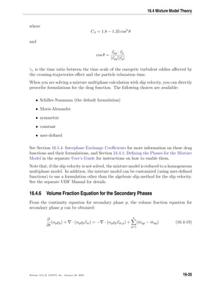
![Multiphase Flows
16.4.7 Granular Properties
Since the concentration of particles is an important factor in the calculation of the effec-
tive viscosity for the mixture, we may use the granular viscosity to get a value for the
viscosity of the suspension. The volume weighted averaged for the viscosity would now
contain shear viscosity arising from particle momentum exchange due to translation and
collision.
The collisional and kinetic parts, and the optional frictional part, are added to give the
solids shear viscosity:
µs = µs,col + µs,kin + µs,fr (16.4-20)
Collisional Viscosity
The collisional part of the shear viscosity is modeled as [110, 343]
µs,col =
4
5
αsρsdsg0,ss(1 + ess)
Θs
π
1/2
αs (16.4-21)
Kinetic Viscosity
ANSYS FLUENT provides two expressions for the kinetic viscosity.
The default expression is from Syamlal et al. [343]:
µs,kin =
αsdsρs
√
Θsπ
6 (3 − ess)
1 +
2
5
(1 + ess) (3ess − 1) αsg0,ss (16.4-22)
The following optional expression from Gidaspow et al. [110] is also available:
µs,kin =
10ρsds
√
Θsπ
96αs (1 + ess) g0,ss
1 +
4
5
g0,ssαs (1 + ess)
2
αs (16.4-23)
16-36 Release 12.0 c ANSYS, Inc. January 29, 2009](https://image.slidesharecdn.com/flth-130501182911-phpapp02/85/Flth-564-320.jpg)
![16.4 Mixture Model Theory
16.4.8 Granular Temperature
The viscosities need the specification of the granular temperature for the sth
solids phase.
Here we use an algebraic equation from the granular temperature transport equation. This
is only applicable for dense fluidized beds where the convection and the diffusion term
can be neglected under the premise that production and dissipation of granular energy
are in equilibrium.
0 = (−psI + τs) : vs − γΘs + φls (16.4-24)
where
(−psI + τs) : vs = the generation of energy by the solid stress tensor
γΘs = the collisional dissipation of energy
φls = the energy exchange between the lth
fluid or solid phase and the sth
solid phase
The collisional dissipation of energy, γΘs , represents the rate of energy dissipation within
the sth
solids phase due to collisions between particles. This term is represented by the
expression derived by Lun et al. [208]
γΘm =
12(1 − e2
ss)g0,ss
ds
√
π
ρsα2
sΘ3/2
s (16.4-25)
The transfer of the kinetic energy of random fluctuations in particle velocity from the sth
solids phase to the lth
fluid or solid phase is represented by φls [110]:
φls = −3KlsΘs (16.4-26)
ANSYS FLUENT allows you to solve for the granular temperature with the following
options:
• algebraic formulation (the default)
This is obtained by neglecting convection and diffusion in the transport equation
(Equation 16.4-24) [343].
• constant granular temperature
This is useful in very dense situations where the random fluctuations are small.
• UDF for granular temperature
Release 12.0 c ANSYS, Inc. January 29, 2009 16-37](https://image.slidesharecdn.com/flth-130501182911-phpapp02/85/Flth-565-320.jpg)
![Multiphase Flows
16.4.9 Interfacial Area Concentration
Interfacial area concentration is defined as the interfacial area between two phases per
unit mixture volume. This is an important parameter for predicting mass, momentum
and energy transfers through the interface between the phases. In two-fluid flow systems,
one discrete (particles) and one continuous, the size and its distribution of the discrete
phase or particles can change rapidly due to growth (mass transfer between phases), ex-
pansion due to pressure changes, coalescence, breakage and/or nucleation mechanisms.
The Population Balance model (see the separate Population Balance Module Manual)
ideally captures this phenomenon, but is computationally expensive since several trans-
port equations need to be solved using moment methods, or more if the discrete method
is used. The interfacial area concentration model uses a single transport equation per
secondary phase and is specific to bubbly flows in liquid at this stage.
The transport equation for the interfacial area concentration can be written as
∂(ρgχp)
∂t
+ · (ρgugχp) =
1
3
Dρg
Dt
χp +
2
3
˙mg
αg
χp + ρg(SRC + SWE + STI) (16.4-27)
where χp is the interfacial area concentration (m2
/m3
), and αg is the gas volume fraction.
The first two terms on the right hand side of Equation 16.4-27 are of gas bubble expansion
due to compressibility and mass transfer (phase change). ˙mg is the mass transfer rate into
the gas phase per unit mixture volume (kg/m3
/s). SRC and SWE are the coalescence sink
terms due to random collision and wake entrainment, respectively. STI is the breakage
source term due to turbulent impact.
Two sets of models, the Hibiki-Ishii model [129] and the Ishii-Kim model [281, 139], exist
for those source and sink terms for the interfacial area concentration, which are based
on the works of Ishii et al. [129, 281]. According to their study, the mechanisms of
interactions can be summarized in five categories:
• Coalescence due to random collision driven by turbulence.
• Breakage due to the impact of turbulent eddies.
• Coalescence due to wake entrainment.
• Shearing-off of small bubbles from large cap bubbles.
• Breakage of large cap bubbles due to flow instability on the bubble surface.
In ANSYS FLUENT, only the first three effects will be considered.
16-38 Release 12.0 c ANSYS, Inc. January 29, 2009](https://image.slidesharecdn.com/flth-130501182911-phpapp02/85/Flth-566-320.jpg)
![16.4 Mixture Model Theory
Hibiki-Ishii Model
SRC = −
1
3φ
(
αg
χp
)2
fcnbλc (16.4-28)
= −(
αg
χp
)2 Γcαg
2 1/3
db
11/3
(αgmax − αg)
exp(−Kc
db
5/6
ρf
1/2 1/3
σ1/2
)
= −
Γc
ψ11/3
1/3
(αgmax − αg)
αg
1/3
χp
5/3
exp[−Kcψ5/6 ρf
1/2 1/3
σ1/2
(
αg
χp
)
5/6
]
where fc, λc and nb are the frequency of particle/bubble collision, the efficiency of coa-
lescence from the collision, and the number of particles per unit mixture volume, respec-
tively. The averaged size of the particle/bubble db is assumed to be calculated as
db = ψ
αg
χp
(16.4-29)
and
λc = exp(−Kc
db
5/6
ρf
1/2 1/3
σ1/2
) (16.4-30)
STI =
1
3φ
(
αg
χp
)2
fBneλB (16.4-31)
= (
αg
χp
)2 ΓBαg(1 − αg) 1/3
db
11/3
(αgmax − αg)
exp(−KB
σ
ρf db
5/3 2/3
)
=
ΓB
ψ11/3
(1 − αg) 1/3
χp
5/3
αg
2/3(αgmax − αg)
exp[−
KB
ψ5/3
σ
ρf
2/3
(
χp
αg
)5/3
]
where fB, λB and ne are the frequency of collision between particles/bubbles and tur-
bulent eddies of the primary phase, the efficiency of breakage from the impact, and the
number of turbulent eddies per unit mixture volume, respectively. In Equation 16.4-31
λB = exp(−KB
σ
ρf db
5/3 2/3
) (16.4-32)
The experimental adjustable coefficients are given as follows:
ΓC = 0.188; KC = 0.129; ΓB = 0.264; KB = 1.37 .
The shape factor ψ is given as 6 and φ as 1
36π
for spherical particles/bubbles. There is
no model for SWE in the Hibiki-Ishii formulation.
Release 12.0 c ANSYS, Inc. January 29, 2009 16-39](https://image.slidesharecdn.com/flth-130501182911-phpapp02/85/Flth-567-320.jpg)
![Multiphase Flows
Ishii-Kim Model
SRC = −
1
3φ
(
αg
χp
)2
CRC[
nb
2
utdb
2
αgmax
1/3(αgmax
1/3 − αg
1/3)
] (16.4-33)
[1 − exp(−C
αgmax
1/3
αg
1/3
αgmax
1/3 − αg
1/3
)]
= −
1
3π
CRCutχp
2
[
1
αgmax
1/3(αgmax
1/3 − αg
1/3)
][1 − exp(−C
αgmax
1/3
αg
1/3
αgmax
1/3 − αg
1/3
)]
SWE = −
1
3φ
(
αg
χp
)2
nb
2
db
2
urCD
1/3
= −
1
3π
CWEurχp
2
CD
1/3
(16.4-34)
STI =
1
3φ
(
αg
χp
)2
CTI(
nbut
db
)(1 −
Wecr
We
)1/2
exp(−
Wecr
We
) (16.4-35)
=
1
18
CTIut
χp
2
αg
(1 −
Wecr
We
)1/2
exp(−
Wecr
We
)
where the mean bubble fluctuating velocity, ut , is given by 1/3
db
1/3
. The bubble terminal
velocity, ur , is a function of the bubble diameter and local time-averaged void fraction.
ur = (
dbg∆ρ
3CDρf
)1/2
(16.4-36)
CD = 24
(1 + 0.1ReD
0.75
)
ReD
and ReD ≡
ρf urdb
µf
(1 − αg) (16.4-37)
We =
ρf ut
2
db
σ
(16.4-38)
where µf is the molecular viscosity of the fluid phase, g is the gravitational acceleration
and σ is the interfacial tension. In this model, when the Weber number, We, is less
than the critical Weber number, Wecr, the breakage rate equals zero, i.e. STI = 0. The
coefficients used are given as follows [139]:
CRC = 0.004
CWE = 0.002
CTI = 0.085
C = 3.0
Wecr = 6.0
αgmax = 0.75
16-40 Release 12.0 c ANSYS, Inc. January 29, 2009](https://image.slidesharecdn.com/flth-130501182911-phpapp02/85/Flth-568-320.jpg)
![16.5 Eulerian Model Theory
Limitations
All other features available in ANSYS FLUENT can be used in conjunction with the
Eulerian multiphase model, except for the following limitations:
• The Reynolds Stress turbulence model is not available on a per phase basis.
• Particle tracking (using the Lagrangian dispersed phase model) interacts only with
the primary phase.
• Streamwise periodic flow with specified mass flow rate cannot be modeled when
the Eulerian model is used (the user is allowed to specify a pressure drop).
• Inviscid flow is not allowed.
• Melting and solidification are not allowed.
• When tracking particles in parallel, the DPM model cannot be used with the Eule-
rian multiphase model if the shared memory option is enabled (Section 23.8: Parallel
Processing for the Discrete Phase Model in the separate User’s Guide). (Note that
using the message passing option, when running in parallel, enables the compati-
bility of all multiphase flow models with the DPM model.)
To change from a single-phase model, where a single set of conservation equations for
momentum, continuity and (optionally) energy is solved, to a multiphase model, addi-
tional sets of conservation equations must be introduced. In the process of introduc-
ing additional sets of conservation equations, the original set must also be modified.
The modifications involve, among other things, the introduction of the volume fractions
α1, α2, . . . αn for the multiple phases, as well as mechanisms for the exchange of momen-
tum, heat, and mass between the phases.
16.5.2 Volume Fraction Equation
The description of multiphase flow as interpenetrating continua incorporates the concept
of phasic volume fractions, denoted here by αq. Volume fractions represent the space
occupied by each phase, and the laws of conservation of mass and momentum are satisfied
by each phase individually. The derivation of the conservation equations can be done by
ensemble averaging the local instantaneous balance for each of the phases [5] or by using
the mixture theory approach [31].
Release 12.0 c ANSYS, Inc. January 29, 2009 16-43](https://image.slidesharecdn.com/flth-130501182911-phpapp02/85/Flth-571-320.jpg)
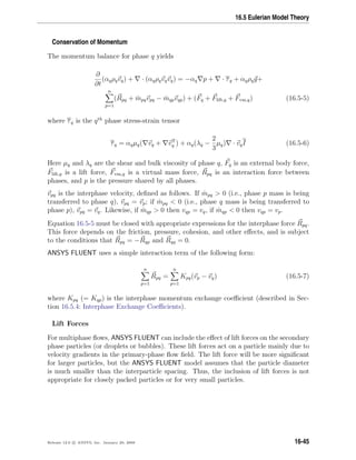
![Multiphase Flows
The lift force acting on a secondary phase p in a primary phase q is computed from [80]
Flift = −0.5ρqαp(vq − vp) × ( × vq) (16.5-8)
The lift force Flift will be added to the right-hand side of the momentum equation for
both phases (Flift,q = −Flift,p).
In most cases, the lift force is insignificant compared to the drag force, so there is no
reason to include this extra term. If the lift force is significant (e.g., if the phases separate
quickly), it may be appropriate to include this term. By default, Flift is not included.
The lift force and lift coefficient can be specified for each pair of phases, if desired.
i It is important that if you include the lift force in your calculation, you
need not include it everywhere in the computational domain since it is
computationally expensive to converge. For example, in the wall boundary
layer for turbulent bubbly flows in channels, the lift force is significant
when the slip velocity is large in the vicinity of high strain rates for the
primary phase.
Virtual Mass Force
For multiphase flows, ANSYS FLUENT includes the “virtual mass effect” that occurs
when a secondary phase p accelerates relative to the primary phase q. The inertia of the
primary-phase mass encountered by the accelerating particles (or droplets or bubbles)
exerts a “virtual mass force” on the particles [80]:
Fvm = 0.5αpρq
dqvq
dt
−
dpvp
dt
(16.5-9)
The term dq
dt
denotes the phase material time derivative of the form
dq(φ)
dt
=
∂(φ)
∂t
+ (vq · )φ (16.5-10)
The virtual mass force Fvm will be added to the right-hand side of the momentum equation
for both phases (Fvm,q = −Fvm,p).
The virtual mass effect is significant when the secondary phase density is much smaller
than the primary phase density (e.g., for a transient bubble column). By default, Fvm is
not included.
16-46 Release 12.0 c ANSYS, Inc. January 29, 2009](https://image.slidesharecdn.com/flth-130501182911-phpapp02/85/Flth-574-320.jpg)
![Multiphase Flows
Fluid-Fluid Momentum Equations
The conservation of momentum for a fluid phase q is
∂
∂t
(αqρqvq) + · (αqρqvqvq) = −αq p + · τq + αqρqg +
n
p=1
(Kpq(vp − vq) + ˙mpqvpq − ˙mqpvqp) +
(Fq + Flift,q + Fvm,q) (16.5-13)
Here g is the acceleration due to gravity and τq, Fq, Flift,q, and Fvm,q are as defined for
Equation 16.5-5.
Fluid-Solid Momentum Equations
Following the work of [3, 49, 71, 110, 183, 208, 254, 343], ANSYS FLUENT uses a multi-
fluid granular model to describe the flow behavior of a fluid-solid mixture. The solid-phase
stresses are derived by making an analogy between the random particle motion arising
from particle-particle collisions and the thermal motion of molecules in a gas, taking into
account the inelasticity of the granular phase. As is the case for a gas, the intensity of the
particle velocity fluctuations determines the stresses, viscosity, and pressure of the solid
phase. The kinetic energy associated with the particle velocity fluctuations is represented
by a “pseudothermal” or granular temperature which is proportional to the mean square
of the random motion of particles.
The conservation of momentum for the fluid phases is similar to Equation 16.5-13, and
that for the sth
solid phase is
∂
∂t
(αsρsvs) + · (αsρsvsvs) = −αs p − ps + · τs + αsρsg +
N
l=1
(Kls(vl − vs) + ˙mlsvls − ˙mslvsl) +
(Fs + Flift,s + Fvm,s) (16.5-14)
where ps is the sth
solids pressure, Kls = Ksl is the momentum exchange coefficient
between fluid or solid phase l and solid phase s, N is the total number of phases, and
Fq, Flift,q, and Fvm,q are as defined for Equation 16.5-5.
16-48 Release 12.0 c ANSYS, Inc. January 29, 2009](https://image.slidesharecdn.com/flth-130501182911-phpapp02/85/Flth-576-320.jpg)
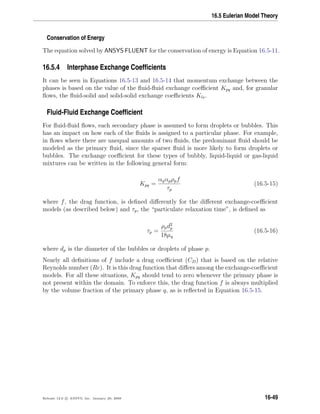
![Multiphase Flows
• For the model of Schiller and Naumann [305]
f =
CDRe
24
(16.5-17)
where
CD =
24(1 + 0.15 Re0.687
)/Re Re ≤ 1000
0.44 Re 1000
(16.5-18)
and Re is the relative Reynolds number. The relative Reynolds number for the
primary phase q and secondary phase p is obtained from
Re =
ρq|vp − vq|dp
µq
(16.5-19)
The relative Reynolds number for secondary phases p and r is obtained from
Re =
ρrp|vr − vp|drp
µrp
(16.5-20)
where µrp = αpµp + αrµr is the mixture viscosity of the phases p and r.
The Schiller and Naumann model is the default method, and it is acceptable for
general use for all fluid-fluid pairs of phases.
• For the Morsi and Alexander model [238]
f =
CDRe
24
(16.5-21)
where
CD = a1 +
a2
Re
+
a3
Re2 (16.5-22)
16-50 Release 12.0 c ANSYS, Inc. January 29, 2009](https://image.slidesharecdn.com/flth-130501182911-phpapp02/85/Flth-578-320.jpg)
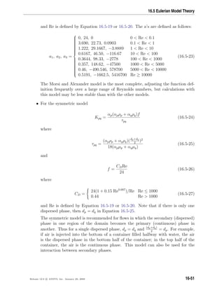
![Multiphase Flows
You can specify different exchange coefficients for each pair of phases. It is also possible
to use user-defined functions to define exchange coefficients for each pair of phases. If the
exchange coefficient is equal to zero (i.e., if no exchange coefficient is specified), the flow
fields for the fluids will be computed independently, with the only “interaction” being
their complementary volume fractions within each computational cell.
Fluid-Solid Exchange Coefficient
The fluid-solid exchange coefficient Ksl can be written in the following general form:
Ksl =
αsρsf
τs
(16.5-28)
where f is defined differently for the different exchange-coefficient models (as described
below), and τs, the “particulate relaxation time”, is defined as
τs =
ρsd2
s
18µl
(16.5-29)
where ds is the diameter of particles of phase s.
All definitions of f include a drag function (CD) that is based on the relative Reynolds
number (Res). It is this drag function that differs among the exchange-coefficient models.
• For the Syamlal-O’Brien model [342]
f =
CDResαl
24v2
r,s
(16.5-30)
where the drag function has a form derived by Dalla Valle [66]
CD =
0.63 +
4.8
Res/vr,s
2
(16.5-31)
This model is based on measurements of the terminal velocities of particles in
fluidized or settling beds, with correlations that are a function of the volume fraction
and relative Reynolds number [294]:
Res =
ρlds|vs − vl|
µl
(16.5-32)
where the subscript l is for the lth
fluid phase, s is for the sth
solid phase, and ds is
the diameter of the sth
solid phase particles.
16-52 Release 12.0 c ANSYS, Inc. January 29, 2009](https://image.slidesharecdn.com/flth-130501182911-phpapp02/85/Flth-580-320.jpg)
![16.5 Eulerian Model Theory
The fluid-solid exchange coefficient has the form
Ksl =
3αsαlρl
4v2
r,sds
CD
Res
vr,s
|vs − vl| (16.5-33)
where vr,s is the terminal velocity correlation for the solid phase [105]:
vr,s = 0.5 A − 0.06 Res + (0.06 Res)2
+ 0.12 Res (2B − A) + A2 (16.5-34)
with
A = α4.14
l (16.5-35)
and
B = 0.8α1.28
l (16.5-36)
for αl ≤ 0.85, and
B = α2.65
l (16.5-37)
for αl 0.85.
This model is appropriate when the solids shear stresses are defined according to
Syamlal et al. [343] (Equation 16.5-83).
• For the model of Wen and Yu [373], the fluid-solid exchange coefficient is of the
following form:
Ksl =
3
4
CD
αsαlρl|vs − vl|
ds
α−2.65
l (16.5-38)
where
CD =
24
αlRes
1 + 0.15(αlRes)0.687
(16.5-39)
and Res is defined by Equation 16.5-32.
This model is appropriate for dilute systems.
Release 12.0 c ANSYS, Inc. January 29, 2009 16-53](https://image.slidesharecdn.com/flth-130501182911-phpapp02/85/Flth-581-320.jpg)
![Multiphase Flows
• The Gidaspow model [110] is a combination of the Wen and Yu model [373] and
the Ergun equation [88].
When αl 0.8, the fluid-solid exchange coefficient Ksl is of the following form:
Ksl =
3
4
CD
αsαlρl|vs − vl|
ds
α−2.65
l (16.5-40)
where
CD =
24
αlRes
1 + 0.15(αlRes)0.687
(16.5-41)
When αl ≤ 0.8,
Ksl = 150
αs(1 − αl)µl
αld2
s
+ 1.75
ρlαs|vs − vl|
ds
(16.5-42)
This model is recommended for dense fluidized beds.
Solid-Solid Exchange Coefficient
The solid-solid exchange coefficient Kls has the following form [341]:
Kls =
3 (1 + els) π
2
+ Cfr,ls
π2
8
αsρsαlρl (dl + ds)2
g0,ls
2π (ρld3
l + ρsd3
s)
|vl − vs| (16.5-43)
where
els = the coefficient of restitution
Cfr,ls = the coefficient of friction between the lth
and sth
solid-phase particles (Cfr,ls = 0)
dl = the diameter of the particles of solid l
g0,ls = the radial distribution coefficient
Note that the coefficient of restitution is described in Section 16.5.5: Solids Pressure
and the radial distribution coefficient is described in Section 16.5.5: Radial Distribution
Function.
16-54 Release 12.0 c ANSYS, Inc. January 29, 2009](https://image.slidesharecdn.com/flth-130501182911-phpapp02/85/Flth-582-320.jpg)
![16.5 Eulerian Model Theory
Universal Drag Laws for Bubble-Liquid and Droplet-Gas Flows
The universal drag laws [170] are suitable for the calculation of the drag coefficients
in bubble-liquid or droplet-gas flow regimes. The drag laws can apply to non-spherical
particles with the constraint of a pool flow regime, i.e. the hydraulic diameter of the flow
domain which is far larger than the averaged size of the particles.
The exchange coefficient for bubbly and droplet flows can be written in the general form
Kpq =
αqαpρpf
τp
(16.5-44)
Where q represents the primary phase and p the particulate phase. The particulate
relaxation time τp is defined as
τp =
ρpdp
2
18µe
(16.5-45)
The drag function f is defined as
f =
CDRe
24
(16.5-46)
The relative Reynolds number for the primary phase q and the secondary phase p is
obtained based on the relative velocity of the two phases.
Re =
ρq|vq − vp|dp
µe
(16.5-47)
Where µe is the effective viscosity of the primary phase accounting for the effects of
family of particles in the continuum.
The Rayleigh-Taylor instability wavelength is
λRT =
σ
g∆ρpq
0.5
(16.5-48)
Where σ is the surface tension, g the gravity, and ∆ρpq the absolute value of the density
difference between phases p and q.
The drag coefficient is defined differently for bubbly and droplet flows.
Release 12.0 c ANSYS, Inc. January 29, 2009 16-55](https://image.slidesharecdn.com/flth-130501182911-phpapp02/85/Flth-583-320.jpg)
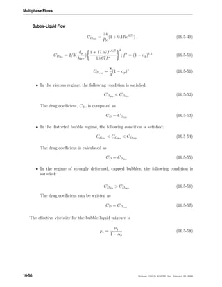
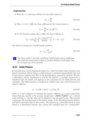
![Multiphase Flows
condition with α αs,max, where the spacing between the solid particles can continue to
decrease, to the “incompressible” condition with α = αs,max, where no further decrease
in the spacing can occur. A value of 0.63 is the default for αs,max, but you can modify it
during the problem setup.
Other formulations that are also available in ANSYS FLUENT are [343]
ps = 2ρs(1 + ess)α2
sg0,ssΘs (16.5-64)
and [213]
ps = αsρsΘs[(1 + 4αsg0,ss) +
1
2
[(1 + ess)(1 − ess + 2µfric)]] (16.5-65)
When more than one solids phase are calculated, the above expression does not take into
account the effect of other phases. A derivation of the expressions from the Boltzman
equations for a granular mixture are beyond the scope of this manual, however there is
a need to provide a better formulation so that some properties may feel the presence of
other phases. A known problem is that N solid phases with identical properties should be
consistent when the same phases are described by a single solids phase. Equations derived
empirically may not satisfy this property and need to be changed accordingly without
deviating significantly from the original form. From [109], a general solids pressure
formulation in the presence of other phases could be of the form
pq = αqρqΘq +
N
p=1
π
3
g0,pqd3
qpnqnp(1 + eqp)f(mp, mq, Θp, Θq) (16.5-66)
where dpq = dp+dq
2
is the average diameter, np, nq are the number of particles, mp and mq
are the masses of the particles in phases p and q, and f is a function of the masses of the
particles and their granular temperatures. For now, we have to simplify this expression
so that it depends only on the granular temperature of phase q
pq = αqρqΘq +
N
p=1
2
d3
pq
d3
q
(1 + epq)g0,pqαqαpρqΘq (16.5-67)
Since all models need to be cast in the general form, it follows that
pq = αqρqΘq + (
N
p=1
d3
pq
d3
q
pc,qp)ρqΘq (16.5-68)
where pc,qp is the collisional part of the pressure between phases q and p.
The above expression reverts to the one solids phase expression when N = 1 and q = p
but also has the property of feeling the presence of other phases.
16-58 Release 12.0 c ANSYS, Inc. January 29, 2009](https://image.slidesharecdn.com/flth-130501182911-phpapp02/85/Flth-586-320.jpg)
![16.5 Eulerian Model Theory
Radial Distribution Function
The radial distribution function, g0, is a correction factor that modifies the probability
of collisions between grains when the solid granular phase becomes dense. This function
may also be interpreted as the nondimensional distance between spheres:
g0 =
s + dp
s
(16.5-69)
where s is the distance between grains. From Equation 16.5-69 it can be observed that
for a dilute solid phase s → ∞, and therefore g0 → 1. In the limit when the solid phase
compacts, s → 0 and g0 → ∞. The radial distribution function is closely connected
to the factor χ of Chapman and Cowling’s [49] theory of nonuniform gases. χ is equal
to 1 for a rare gas, and increases and tends to infinity when the molecules are so close
together that motion is not possible.
In the literature there is no unique formulation for the radial distribution function. AN-
SYS FLUENT has a number of options:
• For one solids phase, use [254]:
g0 =
1 −
αs
αs,max
1
3
−1
(16.5-70)
This is an empirical function and does not extend easily to n phases. For two
identical phases with the property that αq = α1 + α2, the above function is not
consistent for the calculation of the partial pressures p1 and p2, pq = p1+p2. In order
to correct this problem, ANSYS FLUENT uses the following consistent formulation:
g0,ll =
1 −
αs
αs,max
1
3
−1
+
1
2
dl
N
k=1
αk
dk
(16.5-71)
where
αs =
N
k=1
αk (16.5-72)
and k are solid phases only.
• The following expression is also available [137]:
g0,ll =
1
(1 − αs
αs,max
)
+
3
2
dl
N
k=1
αk
dk
(16.5-73)
Release 12.0 c ANSYS, Inc. January 29, 2009 16-59](https://image.slidesharecdn.com/flth-130501182911-phpapp02/85/Flth-587-320.jpg)
![Multiphase Flows
• Also available [213], slightly modified for n solids phases, is the following:
g0,ll =
1 + 2.5αs + 4.59α2
s + 4.52α3
s
1 − αs
αs,max
3 0.678 +
1
2
dl
N
k=1
αk
dk
(16.5-74)
• The following equation [343] is available:
g0,kl =
1
(1 − αs)
+
3( N
k=1
αk
dk
)
(1 − αs)2(dj + dk)
dkdl (16.5-75)
When the number of solid phases is greater than 1, Equation 16.5-71, Equation 16.5-73
and Equation 16.5-74 are extended to
g0,lm =
dmg0,ll + dlg0,mm
dm + dl
(16.5-76)
It is interesting to note that Equation 16.5-73 and Equation 16.5-74 compare well with [3]
experimental data, while Equation 16.5-75 reverts to the [46] derivation.
16.5.6 Maximum Packing Limit in Binary Mixtures
The packing limit is not a fixed quantity and may change according to the number of
particles present within a given volume and the diameter of the particles. Small particles
accumulate in between larger particles increasing the packing limit. For a binary mixture
ANSYS FLUENT uses the correlations proposed by [90].
For a binary mixture with diameters d1 d2, the mixture composition is defined as
X1 = α1
α1+α2
where
X1 =
α1,max
(α1,max + (1 − α1,max)α2,max)
(16.5-77)
as this is a condition for application of the maximum packing limit for binary mixtures.
The maximum packing limit for the mixture is given by
αs,max = (α1,max − α2,max + [1 −
d2
d1
](1 − α1,max)α2,max) (16.5-78)
∗(α1,max + (1 − α1,max)α2,max)
X1
α1,max
+α2,max (16.5-79)
16-60 Release 12.0 c ANSYS, Inc. January 29, 2009](https://image.slidesharecdn.com/flth-130501182911-phpapp02/85/Flth-588-320.jpg)
α2,max)(1 − X1) + α1,max (16.5-80)
The packing limit is used for the calculation of the radial distribution function.
16.5.7 Solids Shear Stresses
The solids stress tensor contains shear and bulk viscosities arising from particle momen-
tum exchange due to translation and collision. A frictional component of viscosity can
also be included to account for the viscous-plastic transition that occurs when particles
of a solid phase reach the maximum solid volume fraction.
The collisional and kinetic parts, and the optional frictional part, are added to give the
solids shear viscosity:
µs = µs,col + µs,kin + µs,fr (16.5-81)
Collisional Viscosity
The collisional part of the shear viscosity is modeled as [110, 343]
µs,col =
4
5
αsρsdsg0,ss(1 + ess)
Θs
π
1/2
αs (16.5-82)
Kinetic Viscosity
ANSYS FLUENT provides two expressions for the kinetic part.
The default expression is from Syamlal et al. [343]:
µs,kin =
αsdsρs
√
Θsπ
6 (3 − ess)
1 +
2
5
(1 + ess) (3ess − 1) αsg0,ss (16.5-83)
The following optional expression from Gidaspow et al. [110] is also available:
µs,kin =
10ρsds
√
Θsπ
96αs (1 + ess) g0,ss
1 +
4
5
g0,ssαs (1 + ess)
2
αs (16.5-84)
Release 12.0 c ANSYS, Inc. January 29, 2009 16-61](https://image.slidesharecdn.com/flth-130501182911-phpapp02/85/Flth-589-320.jpg)
![Multiphase Flows
Bulk Viscosity
The solids bulk viscosity accounts for the resistance of the granular particles to compres-
sion and expansion. It has the following form from Lun et al. [208]:
λs =
4
3
αsρsdsg0,ss(1 + ess)
Θs
π
1/2
(16.5-85)
Note that the bulk viscosity is set to a constant value of zero, by default. It is also
possible to select the Lun et al. expression or use a user-defined function.
Frictional Viscosity
In dense flow at low shear, where the secondary volume fraction for a solid phase nears
the packing limit, the generation of stress is mainly due to friction between particles.
The solids shear viscosity computed by ANSYS FLUENT does not, by default, account
for the friction between particles.
If the frictional viscosity is included in the calculation, ANSYS FLUENT uses Schaef-
fer’s [303] expression:
µs,fr =
ps sin φ
2
√
I2D
(16.5-86)
where ps is the solids pressure, φ is the angle of internal friction, and I2D is the second
invariant of the deviatoric stress tensor. It is also possible to specify a constant or user-
defined frictional viscosity.
In granular flows with high solids volume fraction, instantaneous collisions are less im-
portant. The application of kinetic theory to granular flows is no longer relevant since
particles are in contact and the resulting frictional stresses need to be taken into account.
ANSYS FLUENT extends the formulation of the frictional viscosity and employs other
models, as well as providing new hooks for UDFs. See the separate UDF Manual for
details.
The frictional stresses are usually written in Newtonian form:
τfriction = −PfrictionI + µfriction( us + ( us)T
) (16.5-87)
The frictional stress is added to the stress predicted by the kinetic theory when the solids
volume fraction exceeds a critical value. This value is normally set to 0.5 when the flow
is three-dimensional and the maximum packing limit is about 0.63. Then
PS = Pkinetic + Pfriction (16.5-88)
16-62 Release 12.0 c ANSYS, Inc. January 29, 2009](https://image.slidesharecdn.com/flth-130501182911-phpapp02/85/Flth-590-320.jpg)
![16.5 Eulerian Model Theory
µS = µkinetic + µfriction (16.5-89)
The derivation of the frictional pressure is mainly semi-empirical, while the frictional vis-
cosity can be derived from the first principles. The application of the modified Coulomb
law leads to an expression of the form
µfriction =
Pfriction sin φ
2
√
I2D
(16.5-90)
Where φ is the angle of internal friction and I2D is the second invariant of the deviatoric
stress tensor.
Two additional models are available in ANSYS FLUENT: the Johnson and Jackson [151]
model for frictional pressure and Syamlal et al [343].
The Johnson and Jackson [151] model for frictional pressure is defined as
Pfriction = Fr
(αs − αs,min)n
(αs,max − αs)p
(16.5-91)
With coefficient Fr = 0.05, n=2 and p = 5 [253]. The critical value for the solids volume
fraction is 0.5. The coefficient Fr was modified to make it a function of the volume
fraction:
Fr = 0.1αs (16.5-92)
The frictional viscosity for this model is of the form
µfriction = Pfriction sin φ (16.5-93)
The second model that is employed is Syamlal et al. [343], described in Equation 16.5-83.
Comparing the two models results in the frictional normal stress differing by orders of
magnitude.
Release 12.0 c ANSYS, Inc. January 29, 2009 16-63](https://image.slidesharecdn.com/flth-130501182911-phpapp02/85/Flth-591-320.jpg)
![Multiphase Flows
The radial distribution function is an important parameter in the description of the solids
pressure resulting from granular kinetic theory. If we use the models of Lun et al. [208] or
Gidaspow [109] the radial function tends to infinity as the volume fraction tends to the
packing limit. It would then be possible to use this pressure directly in the calculation
of the frictional viscosity, as it has the desired effect. This approach is also available in
ANSYS FLUENT by default.
i The introduction of the frictional viscosity helps in the description of fric-
tional flows, however a complete description would require the introduction
of more physics to capture the elastic regime with the calculation of the
yield stress and the use of the flow-rule. These effects can be added by the
user via UDFs to model static regime. Small time steps are required to get
good convergence behavior.
16.5.8 Granular Temperature
The granular temperature for the sth
solids phase is proportional to the kinetic energy of
the random motion of the particles. The transport equation derived from kinetic theory
takes the form [71]
3
2
∂
∂t
(ρsαsΘs) + · (ρsαsvsΘs) = (−psI+τs) : vs+ ·(kΘs Θs)−γΘs +φls (16.5-94)
where
(−psI + τs) : vs = the generation of energy by the solid stress tensor
kΘs Θs = the diffusion of energy (kΘs is the diffusion coefficient)
γΘs = the collisional dissipation of energy
φls = the energy exchange between the lth
fluid or solid phase and the sth
solid phase
Equation 16.5-94 contains the term kΘs Θs describing the diffusive flux of granular
energy. When the default Syamlal et al. model [343] is used, the diffusion coefficient for
granular energy, kΘs is given by
kΘs =
15dsρsαs
√
Θsπ
4(41 − 33η)
1 +
12
5
η2
(4η − 3)αsg0,ss +
16
15π
(41 − 33η)ηαsg0,ss) (16.5-95)
where
η =
1
2
(1 + ess)
16-64 Release 12.0 c ANSYS, Inc. January 29, 2009](https://image.slidesharecdn.com/flth-130501182911-phpapp02/85/Flth-592-320.jpg)
![16.5 Eulerian Model Theory
ANSYS FLUENT uses the following expression if the optional model of Gidaspow et
al. [110] is enabled:
kΘs =
150ρsds (Θπ)
384(1 + ess)g0,ss
1 +
6
5
αsg0,ss(1 + es)
2
+ 2ρsαs
2
ds(1 + ess)g0,ss
Θs
π
(16.5-96)
The collisional dissipation of energy, γΘs , represents the rate of energy dissipation within
the sth
solids phase due to collisions between particles. This term is represented by the
expression derived by Lun et al. [208]
γΘm =
12(1 − e2
ss)g0,ss
ds
√
π
ρsα2
sΘ3/2
s (16.5-97)
The transfer of the kinetic energy of random fluctuations in particle velocity from the sth
solids phase to the lth
fluid or solid phase is represented by φls [110]:
φls = −3KlsΘs (16.5-98)
ANSYS FLUENT allows the user to solve for the granular temperature with the following
options:
• algebraic formulation (the default)
It is obtained by neglecting convection and diffusion in the transport equation,
Equation 16.5-94 [343].
• partial differential equation
This is given by Equation 16.5-94 and it is allowed to choose different options for
it properties.
• constant granular temperature
This is useful in very dense situations where the random fluctuations are small.
• UDF for granular temperature
For a granular phase s, we may write the shear force at the wall in the following form:
τs = −
π
6
√
3φ
αs
αs,max
ρsg0 ΘsUs,|| (16.5-99)
Here Us,|| is the particle slip velocity parallel to the wall, φ is the specularity coefficient
between the particle and the wall, αs,max is the volume fraction for the particles at
maximum packing, and g0 is the radial distribution function that is model dependent.
Release 12.0 c ANSYS, Inc. January 29, 2009 16-65](https://image.slidesharecdn.com/flth-130501182911-phpapp02/85/Flth-593-320.jpg)
![Multiphase Flows
The general boundary condition for granular temperature at the wall takes the form
[151]
qs =
π
6
√
3φ
αs
αs,max
ρsg0 Θs)Us,|| · Us,|| −
π
4
√
3
αs
αs,max
(1 − e2
sw)ρsg0Θ
3
2
s (16.5-100)
16.5.9 Interfacial Area Concentration
Interfacial area concentration is defined as the interfacial area between two phases per
unit mixture volume. This is an important parameter for predicting mass, momen-
tum and energy transfers through the interface between the phases. The models that
are inplemented in ANSYS FLUENT are discussed in Section 16.4.9: Interfacial Area
Concentration.
16.5.10 Description of Heat Transfer
The internal energy balance for phase q is written in terms of the phase enthalpy, Equa-
tion 16.5-11, defined by
Hq = cp,qdTq (16.5-101)
where cp,q is the specific heat at constant pressure of phase q. The thermal boundary
conditions used with multiphase flows are the same as those for a single-phase flow. See
Chapter 7: Cell Zone and Boundary Conditions in the separate User’s Guide for details.
The Heat Exchange Coefficient
The rate of energy transfer between phases is assumed to be a function of the temperature
difference
Qpq = hpq(Tp − Tq) (16.5-102)
where hpq(= hqp) is the heat transfer coefficient between the pth
phase and the qth
phase.
The heat transfer coefficient is related to the pth
phase Nusselt number, Nup, by
hpq =
6κqαpαqNup
dp
2 (16.5-103)
Here κq is the thermal conductivity of the qth
phase. The Nusselt number is typically
determined from one of the many correlations reported in the literature. In the case of
fluid-fluid multiphase, ANSYS FLUENT uses the correlation of Ranz and Marshall [284,
285]:
16-66 Release 12.0 c ANSYS, Inc. January 29, 2009](https://image.slidesharecdn.com/flth-130501182911-phpapp02/85/Flth-594-320.jpg)
![16.5 Eulerian Model Theory
Nup = 2.0 + 0.6Re1/2
p Pr1/3
(16.5-104)
where Rep is the relative Reynolds number based on the diameter of the pth
phase and
the relative velocity |up − uq|, and Pr is the Prandtl number of the qth
phase:
Pr =
cpqµq
κq
(16.5-105)
In the case of granular flows (where p = s), ANSYS FLUENT uses a Nusselt number
correlation by Gunn [117], applicable to a porosity range of 0.35–1.0 and a Reynolds
number of up to 105
:
Nus = (7−10αf +5α2
f )(1+0.7Re0.2
s Pr1/3
)+(1.33−2.4αf +1.2α2
f )Re0.7
s Pr1/3
(16.5-106)
The Prandtl number is defined as above with q = f. For all these situations, hpq should
tend to zero whenever one of the phases is not present within the domain. To enforce
this, hpq is always multiplied by the volume fraction of the primary phase q, as reflected
in Equation 16.5-103.
16.5.11 Turbulence Models
To describe the effects of turbulent fluctuations of velocities and scalar quantities in
a single phase, ANSYS FLUENT uses various types of closure models, as described in
Chapter 4: Turbulence. In comparison to single-phase flows, the number of terms to be
modeled in the momentum equations in multiphase flows is large, and this makes the
modeling of turbulence in multiphase simulations extremely complex.
ANSYS FLUENT provides three methods for modeling turbulence in multiphase flows
within the context of the k- models. In addition, ANSYS FLUENT provides two turbu-
lence options within the context of the Reynolds stress models (RSM).
The k- turbulence model options are:
• mixture turbulence model (the default)
• dispersed turbulence model
• turbulence model for each phase
i Note that the descriptions of each method below are presented based on
the standard k- model. The multiphase modifications to the RNG and
realizable k- models are similar, and are therefore not presented explicitly.
Release 12.0 c ANSYS, Inc. January 29, 2009 16-67](https://image.slidesharecdn.com/flth-130501182911-phpapp02/85/Flth-595-320.jpg)
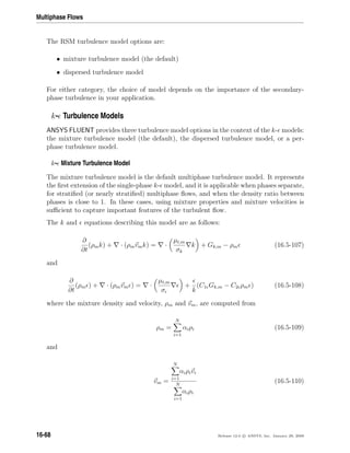
![16.5 Eulerian Model Theory
the turbulent viscosity, µt,m, is computed from
µt,m = ρmCµ
k2
(16.5-111)
and the production of turbulence kinetic energy, Gk,m, is computed from
Gk,m = µt,m( vm + ( vm)T
) : vm (16.5-112)
The constants in these equations are the same as those described in Section 4.4.1: Stan-
dard k- Model for the single-phase k- model.
k- Dispersed Turbulence Model
The dispersed turbulence model is the appropriate model when the concentrations of the
secondary phases are dilute. In this case, interparticle collisions are negligible and the
dominant process in the random motion of the secondary phases is the influence of the
primary-phase turbulence. Fluctuating quantities of the secondary phases can therefore
be given in terms of the mean characteristics of the primary phase and the ratio of the
particle relaxation time and eddy-particle interaction time.
The model is applicable when there is clearly one primary continuous phase and the rest
are dispersed dilute secondary phases.
Assumptions
The dispersed method for modeling turbulence in ANSYS FLUENT assumes the following:
• a modified k- model for the continuous phase
Turbulent predictions for the continuous phase are obtained using the standard
k- model supplemented with extra terms that include the interphase turbulent
momentum transfer.
• Tchen-theory correlations for the dispersed phases
Predictions for turbulence quantities for the dispersed phases are obtained using the
Tchen theory of dispersion of discrete particles by homogeneous turbulence [130].
Release 12.0 c ANSYS, Inc. January 29, 2009 16-69](https://image.slidesharecdn.com/flth-130501182911-phpapp02/85/Flth-597-320.jpg)
![16.5 Eulerian Model Theory
∂
∂t
(αqρqkq) + · (αqρqUqkq) = · (αq
µt,q
σk
kq) + αqGk,q − αqρq q + αqρqΠkq (16.5-117)
and
∂
∂t
(αqρq q) + · (αqρqUq q) = · (αq
µt,q
σ
q) + αq
q
kq
(C1 Gk,q − C2 ρq q) + αqρqΠ q
(16.5-118)
Here Πkq and Π q represent the influence of the dispersed phases on the continuous phase
q, and Gk,q is the production of turbulent kinetic energy, as defined in Section 4.4.4: Mod-
eling Turbulent Production in the k- Models. All other terms have the same meaning
as in the single-phase k- model.
The term Πkq can be derived from the instantaneous equation of the continuous phase
and takes the following form, where M represents the number of secondary phases:
Πkq =
M
p=1
Kpq
αqρq
( vq · vp +(Up − Uq) · vdr) (16.5-119)
which can be simplified to
Πkq =
M
p=1
Kpq
αqρq
(kpq − 2kq + vpq · vdr) (16.5-120)
where klq is the covariance of the velocities of the continuous phase q and the dispersed
phase l (calculated from Equation 16.5-128 below), vpq is the relative velocity, and vdr is
the drift velocity (defined by Equation 16.5-133 below).
Π q is modeled according to Elgobashi et al. [87]:
Π q = C3
q
kq
Πkq (16.5-121)
where C3 = 1.2.
Turbulence in the Dispersed Phase
Time and length scales that characterize the motion are used to evaluate dispersion
coefficients, correlation functions, and the turbulent kinetic energy of each dispersed
phase.
Release 12.0 c ANSYS, Inc. January 29, 2009 16-71](https://image.slidesharecdn.com/flth-130501182911-phpapp02/85/Flth-599-320.jpg)
![Multiphase Flows
The characteristic particle relaxation time connected with inertial effects acting on a
dispersed phase p is defined as
τF,pq = αpρqK−1
pq
ρp
ρq
+ CV (16.5-122)
The Lagrangian integral time scale calculated along particle trajectories, mainly affected
by the crossing-trajectory effect [63], is defined as
τt,pq =
τt,q
(1 + Cβξ2)
(16.5-123)
where
ξ =
|vpq|τt,q
Lt,q
(16.5-124)
and
Cβ = 1.8 − 1.35 cos2
θ (16.5-125)
where θ is the angle between the mean particle velocity and the mean relative velocity.
The ratio between these two characteristic times is written as
ηpq =
τt,pq
τF,pq
(16.5-126)
Following Simonin [317], ANSYS FLUENT writes the turbulence quantities for dispersed
phase p as follows:
kp = kq
b2
+ ηpq
1 + ηpq
(16.5-127)
kpq = 2kq
b + ηpq
1 + ηpq
(16.5-128)
Dt,pq =
1
3
kpqτt,pq (16.5-129)
Dp = Dt,pq +
2
3
kp − b
1
3
kpq τF,pq (16.5-130)
b = (1 + CV )
ρp
ρq
+ CV
−1
(16.5-131)
and CV = 0.5 is the added-mass coefficient.
16-72 Release 12.0 c ANSYS, Inc. January 29, 2009](https://image.slidesharecdn.com/flth-130501182911-phpapp02/85/Flth-600-320.jpg)
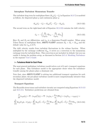
![16.5 Eulerian Model Theory
RSM Turbulence Models
Multiphase turbulence modeling typically involves two equation models that are based
on single-phase models and often cannot accurately capture the underlying flow physics.
Additional turbulence modeling for multiphase flows is diminished even more when the
basic underlying single-phase model cannot capture the complex physics of the flow. In
such situations, the logical next step is to combine the Reynolds stress model with the
multiphase algorithm in order to handle challenging situations in which both factors,
RSM for turbulence and the Eulerian multiphase formulation, are a precondition for
accurate predictions [59].
The phase-averaged continuity and momentum equations for a continuous phase are:
∂
∂t
(αcρc) + · (αcρc
˜Uc) = 0 (16.5-138)
∂
∂t
(αcρrmc
˜Uc) + · (αcρrmc
˜Uc
˜Uc) = −αc ˜p + · ˜τt
c + FDc (16.5-139)
For simplicity, the laminar stress-strain tensor and other body forces such as gravity
have been omitted from Equations 16.5-138-16.5-139. The tilde denotes phase-averaged
variables while an overbar (e.g., αc) reflects time-averaged values. In general, any variable
Φ can have a phase-average value defined as
˜Φc =
αcΦc
αc
(16.5-140)
Considering only two phases for simplicity, the drag force between the continuous and
the dispersed phases can be defined as:
FDc = Kdc ( ˜Ud − ˜Uc) −
αdud
αd
−
αcuc
αc
(16.5-141)
where Kdc is the drag coefficient. Several terms in the Equation 16.5-141 need to be
modeled in order to close the phase-averaged momentum equations. Full descriptions of
all modeling assumptions can be found in [58]. This section only describes the different
modeling definition of the turbulent stresses ˜τt that appears in Equation 16.5-139.
The turbulent stress that appears in the momentum equations need to be defined on a
per-phase basis and can be calculated as:
˜τt
k = −αkρk
˜Rk,ij (16.5-142)
Release 12.0 c ANSYS, Inc. January 29, 2009 16-75](https://image.slidesharecdn.com/flth-130501182911-phpapp02/85/Flth-603-320.jpg)
![Multiphase Flows
where the subscript k is replaced by c for the primary (i.e., continuous) phase or by
d for any secondary (i.e., dispersed) phases. As is the case for single-phase flows, the
current multiphase Reynolds stress model (RSM) also solves the transport equations for
Reynolds stresses Rij. ANSYS FLUENT includes two methods for modeling turbulence in
multiphase flows within the context of the RSM model: the dispersed turbulence model,
and the mixture turbulence model.
RSM Dispersed Turbulence Model
The dispersed turbulence model is used when the concentrations of the secondary phase
are dilute and the primary phase turbulence is regarded as the dominant process. Conse-
quently, the transport equations for turbulence quantities are only solved for the primary
(continuous) phase, while the predictions of turbulence quantities for dispersed phases
are obtained using the Tchen theory. The transport equation for the primary phase
Reynolds stresses in the case of the dispersed model are:
∂
∂t
(αρ ˜Rij) +
∂
∂xk
(αρ ˜Uk
˜Rij) = −αρ ˜Rik
∂ ˜Uj
∂xk
+ ˜Rjk
∂ ˜Ui
∂xk
+
∂
∂xk
αµ
∂
∂xk
( ˜Rij)
−
∂
∂xk
[αρuiujuk] + αp(
∂ui
∂xj
+
∂uj
∂xi
)
− αρ ˜ij + ΠR,ij (16.5-143)
The variables in Equation 16.5-143 are per continuous phase c and the subscript is omitted
for clarity. The last term of Equation 16.5-143, ΠR,ij, takes into account the interaction
between the continuous and the dispersed phase turbulence. A general model for this
term can be of the form:
ΠR,ij = KdcC1,dc(Rdc,ij − Rc,ij) + KdcC2,dcadc,ibdc,j (16.5-144)
where C1 and C2 are unknown coefficients, adc,i is the relative velocity, bdc,j represents
the drift or the relative velocity, and Rdc,ij is the unknown particulate-fluid velocity
correlation. To simplify this unknown term, the following assumption has been made:
ΠR,ij =
2
3
δijΠk (16.5-145)
where δij is the Kronecker delta, and Πk represents the modified version of the original
Simonin model [317].
Πkc = Kdc(˜kdc − 2˜kc + ˜Vrel · ˜Vdrift) (16.5-146)
16-76 Release 12.0 c ANSYS, Inc. January 29, 2009](https://image.slidesharecdn.com/flth-130501182911-phpapp02/85/Flth-604-320.jpg)
![16.5 Eulerian Model Theory
where ˜Kc represents the turbulent kinetic energy of the continuous phase, ˜kdc is the
continuous-dispersed phase velocity covariance and finally, ˜Vrel and ˜Vdrift stand for the
relative and the drift velocities, respectively. In order to achieve full closure, the transport
equation for the turbulent kinetic energy dissipation rate (˜) is required. The modeling
of ˜ together with all other unknown terms in Equation 16.5-146 are modeled in the same
way as in [58].
RSM Mixture Turbulence Model
The main assumption for the mixture model is that all phases share the same turbu-
lence field which consequently means that the term ΠR in the Reynolds stress transport
equations (Equation 16.5-143) is neglected. Apart from that, the equations maintain the
same form but with phase properties and phase velocities being replaced with mixture
properties and mixture velocities. The mixture density, for example, can be expressed as
ρm =
N
i=1
αiρi (16.5-147)
while mixture velocities can be expressed as
˜Um =
N
i=1 αiρi
˜Ui
N
i=1 αiρi
(16.5-148)
where N is the number of species.
16.5.12 Solution Method in ANSYS FLUENT
For Eulerian multiphase calculations, ANSYS FLUENT can solve the phase momentum
equations, the shared pressure, and phasic volume fraction equations in a coupled and
segregated fashion. The coupled solution for multiphase flows is discussed in detail in Sec-
tion 24.7.1: Coupled Solution for Multiphase Flows in the separate User’s Guide. When
solving the equations in a segregated manner, ANSYS FLUENT uses the phase coupled
SIMPLE (PC-SIMPLE) algorithm [354] for the pressure-velocity coupling. PC-SIMPLE
is an extension of the SIMPLE algorithm [264] to multiphase flows. The velocities are
solved coupled by phases, but in a segregated fashion. The block algebraic multigrid
scheme used by the density-based solver described in [371] is used to solve a vector equa-
tion formed by the velocity components of all phases simultaneously. Then, a pressure
correction equation is built based on total volume continuity rather than mass continuity.
Pressure and velocities are then corrected so as to satisfy the continuity constraint.
Release 12.0 c ANSYS, Inc. January 29, 2009 16-77](https://image.slidesharecdn.com/flth-130501182911-phpapp02/85/Flth-605-320.jpg)
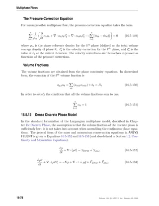
![Multiphase Flows
Limitations
Since the given approach makes use of the Eulerian multiphase model framework, all its
limitations are adopted:
• The turbulence models: LES, DES and k − ω turbulence models are not available.
• The combustion models: PDF Transport model, Premixed, Non-premixed and par-
tially premixed combustion models are not available.
• The radiation models are not available.
• The solidification and melting models are not available.
• The Wet Steam model is not available.
• The real gas model (pressure-based and density-based) is not available.
• The density-based solver and models dependent on it are not available.
• Parallel DPM with the shared memory option is disabled.
Granular Temperature
The solids stress acting on particles in a dense flow situation is modeled via an additional
acceleration in the particle force balance Equation 15.2-1.
dup
dt
= FD (u − up) +
gx (ρp − ρ)
ρp
+ Fx + Finteraction (16.5-156)
The term Finteraction models the additional acceleration acting on a particle, resulting
from interparticle interaction. It is computed from the stress tensor given by the Kinetic
Theory of Granular Flows as
Finteraction = −
1
ρp
· ¯¯τs (16.5-157)
The conservation equation for the granular temperature (kinetic energy of the fluctuating
particle motion) is solved with the averaged particle velocity field. Therefore, a sufficient
statistical representation of the particle phase is needed to ensure the stable behavior
of the granular temperature equation. For details on the Kinetic Theory of Granular
Flows, please refer to Section 16.5.3: Conservation Equations – Section 16.5.8: Granular
Temperature.
The main advantage over the Eulerian model is that, there is no need to define classes
to handle particle size distributions. This is done in a natural way in the Lagrangian
formulation [279].
16-80 Release 12.0 c ANSYS, Inc. January 29, 2009](https://image.slidesharecdn.com/flth-130501182911-phpapp02/85/Flth-608-320.jpg)
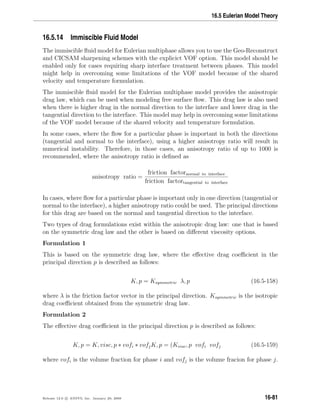
![Multiphase Flows
The viscous drag component in the principal direction Kvisc, p is
Kvisc, p =
µ
(lclc)
λ, p (16.5-160)
where the viscosity options can be any one of the following:
µ = 0.5(µi + µj)
µ = 2µiµj
(µi+µj)
µ = µiµj
(µivofj+µjvofi)
µ = µivofi + µjvofj
µ = µi
µ = µj
and lc is the length scale.
To learn how to use the immiscible fluid model and the two drag formulations, refer to
Section 24.5.8: Including the Immiscible Fluid Model in the separate User’s Guide.
16.6 Wet Steam Model Theory
Information is organized into the following subsections:
• Section 16.6.1: Overview and Limitations of the Wet Steam Model
• Section 16.6.2: Wet Steam Flow Equations
• Section 16.6.3: Phase Change Model
• Section 16.6.4: Built-in Thermodynamic Wet Steam Properties
16.6.1 Overview and Limitations of the Wet Steam Model
Overview
During the rapid expansion of steam, a condensation process will take place shortly
after the state path crosses the vapor-saturation line. The expansion process causes the
super-heated dry steam to first subcool and then nucleate to form a two-phase mixture
of saturated vapor and fine liquid droplets known as wet steam.
Modeling wet steam is very important in the analysis and design of steam turbines. The
increase in steam turbine exit wetness can cause severe erosion to the turbine blades at
the low-pressure stages, and a reduction in aerodynamic efficiency of the turbine stages
operating in the wet steam region [237].
16-82 Release 12.0 c ANSYS, Inc. January 29, 2009](https://image.slidesharecdn.com/flth-130501182911-phpapp02/85/Flth-610-320.jpg)
![Multiphase Flows
The following assumptions are made in this model:
• The velocity slip between the droplets and gaseous-phase is negligible.
• The interactions between droplets are neglected.
• The mass fraction of the condensed phase, β (also known as wetness factor), is
small (β 0.2).
• Since droplet sizes are typically very small (from approximately 0.1 microns to
approximately 100 microns), it is assumed that the volume of the condensed liquid
phase is negligible.
From the preceding assumptions, it follows that the mixture density (ρ) can be related
to the vapor density (ρv) by the following equation:
ρ =
ρv
(1 − β)
(16.6-1)
In addition, the temperature and the pressure of the mixture will be equivalent to the
temperature and pressure of the vapor-phase.
The mixture flow is governed by the compressible Navier-Stokes equations given in vector
form by Equation 18.5-4:
∂W
∂Q
∂
∂t V
Q dV + [F − G] · dA =
V
H dV (16.6-2)
where Q=(P,u,v,w,T) are mixture quantities. The flow equations are solved using the
same density-based solver algorithms employed for general compressible flows.
To model wet steam, two additional transport equations are needed [138]. The first
transport equation governs the mass fraction of the condensed liquid phase (β):
∂ρβ
∂t
+ · (ρ−→v β) = Γ (16.6-3)
where Γ is the mass generation rate due to condensation and evaporation (kg per unit
volume per second). The second transport equation models the evolution of the number
density of the droplets per unit volume:
∂ρη
∂t
+ · (ρ−→v η) = ρI (16.6-4)
where I is the nucleation rate (number of new droplets per unit volume per second).
16-84 Release 12.0 c ANSYS, Inc. January 29, 2009](https://image.slidesharecdn.com/flth-130501182911-phpapp02/85/Flth-612-320.jpg)
![16.6 Wet Steam Model Theory
To determine the number of droplets per unit volume, Equation 16.6-1 and the average
droplet volume Vd are combined in the following expression:
η =
β
(1 − β)Vd(ρl/ρv)
(16.6-5)
where ρl is the liquid density and the average droplet volume is defined as
Vd =
4
3
πr3
d (16.6-6)
where rd is the droplet radius.
Together, Equation 16.6-2, Equation 16.6-3, and Equation 16.6-4 form a closed system
of equations which, along with Equation 16.6-1, permit the calculation of the wet steam
flow field.
16.6.3 Phase Change Model
The following is assumed in the phase change model:
• The condensation is homogeneous (i.e., no impurities present to form nuclei).
• The droplet growth is based on average representative mean radii.
• The droplet is assumed to be spherical.
• The droplet is surrounded by infinite vapor space.
• The heat capacity of the fine droplet is negligible compared with the latent heat
released in condensation.
The mass generation rate Γ in the classical nucleation theory during the nonequilibrium
condensation process is given by the sum of mass increase due to nucleation (the formation
of critically sized droplets) and also due to growth/demise of these droplets [138].
Therefore, Γ is written as:
Γ =
4
3
πρlIr∗
3
+ 4πρlηr2 ∂r
∂t
(16.6-7)
where r is the average radius of the droplet, and r∗ is the Kelvin-Helmholtz critical droplet
radius, above which the droplet will grow and below which the droplet will evaporate.
An expression for r∗ is given by [387].
Release 12.0 c ANSYS, Inc. January 29, 2009 16-85](https://image.slidesharecdn.com/flth-130501182911-phpapp02/85/Flth-613-320.jpg)
![Multiphase Flows
r∗ =
2σ
ρlRT ln S
(16.6-8)
where σ is the liquid surface tension evaluated at temperature T, ρl is the condensed
liquid density (also evaluated at temperature T), and S is the super saturation ratio
defined as the ratio of vapor pressure to the equilibrium saturation pressure:
s =
P
Psat(T)
(16.6-9)
The expansion process is usually very rapid. Therefore, when the state path crosses the
saturated-vapor line, the process will depart from equilibrium, and the supersaturation
ratio S can take on values greater than one.
The condensation process involves two mechanisms, the transfer of mass from the vapor
to the droplets and the transfer of heat from the droplets to the vapor in the form of
latent heat. This energy transfer relation was presented in [385] and used in [138] and
can be written as:
∂r
∂t
=
P
hlvρl
√
2πRT
γ + 1
2γ
Cp(T0 − T) (16.6-10)
where T0 is the droplet temperature.
The classical homogeneous nucleation theory describes the formation of a liquid-phase
in the form of droplets from a supersaturated phase in the absence of impurities or
foreign particles. The nucleation rate described by the steady-state classical homogeneous
nucleation theory [387] and corrected for nonisothermal effects, is given by:
I =
qc
(1 + θ)
ρ2
v
ρl
2σ
Mm
3
π
e
− 4πr∗
2σ
3KbT
(16.6-11)
where qc is evaporation coefficient, kb is the Boltzmann constant, Mm is mass of one
molecule, σ is the liquid surface tension, and ρl is the liquid density at temperature T.
A nonisothermal correction factor, θ, is given by:
θ =
2(γ − 1)
(γ + 1)
hlv
RT
hlv
RT
− 0.5 (16.6-12)
where hlv is the specific enthalpy of evaporation at pressure p and γ is the ratio of specific
heat capacities.
16-86 Release 12.0 c ANSYS, Inc. January 29, 2009](https://image.slidesharecdn.com/flth-130501182911-phpapp02/85/Flth-614-320.jpg)
![16.6 Wet Steam Model Theory
16.6.4 Built-in Thermodynamic Wet Steam Properties
There are many equations that describe the thermodynamic state and properties of steam.
While some of these equations are accurate in generating property tables, they are not
suitable for fast CFD computations. Therefore, ANSYS FLUENT uses a simpler form of
the thermodynamic state equations [386] for efficient CFD calculations that are accurate
over a wide range of temperatures and pressures. These equations are described below.
Equation of State
The steam equation of state used in the solver, which relates the pressure to the vapor
density and the temperature, is given by [386]:
P = ρvRT(1 + Bρv + Cρv
2
) (16.6-13)
where B, and C are the second and the third virial coefficients given by the following
empirical functions:
B = a1(1 +
τ
α
)−1
+ a2eτ
(1 − e−τ
)
5
2 + a3τ (16.6-14)
where B is given in m3
/kg, τ = 1500
T
with T given in Kelvin, α = 10000.0, a1= 0.0015,
a2= -0.000942, and a3= -0.0004882.
C = a(τ − τ0)e−ατ
+ b (16.6-15)
where C is given in m6
/kg2
, τ = T
647.286
with T given in Kelvin, τo= 0.8978, α=11.16,
a= 1.772, and b= 1.5E-06.
The two empirical functions that define the virial coefficients B and C cover the temper-
ature range from 273 K to 1073 K.
The vapor isobaric specific heat capacity Cpv is given by:
Cpv = Cp0(T) + R [(1 − αvT)(B − B1) − B2] ρv + (1 − 2αvT)C + αvTC1 −
C2
2
ρv
2
(16.6-16)
The vapor specific enthalpy, hv is given by:
hv = h0(T) + RT (B − B1)ρv + (C −
C1
2
)ρv
2
(16.6-17)
The vapor specific entropy, sv is given by:
Release 12.0 c ANSYS, Inc. January 29, 2009 16-87](https://image.slidesharecdn.com/flth-130501182911-phpapp02/85/Flth-615-320.jpg)
![Multiphase Flows
sv = s0(T) − R ln ρv + (B + B1)ρv +
(C + C1)
2
ρv
2
(16.6-18)
The isobaric specific heat at zero pressure is defined by the following empirical equation:
Cp0(T) =
i=1
6
aiTi−2
(16.6-19)
where Cp0 is in KJ/kg K, a1 = 46.0, a2 = 1.47276, a3 = 8.38930E-04, a4 = -2.19989E-07,
a5 = 2.46619E-10, and a6 = -9.70466E-14.
and
B1 = T dB
dT
, C1 = T dC
dT
, B2 = T2 dB2
dT2 , and C2 = T2 dC2
dT2 .
Both h0(T) and s0(T) are functions of temperature and they are defined by:
h0(T) = Cp0dT + hc (16.6-20)
s0(T) =
Cp0
T
dT + sc (16.6-21)
where hc and sc are arbitrary constants.
The vapor dynamic viscosity µv and thermal conductivity Ktv are also functions of
temperature and were obtained from [385].
Saturated Vapor Line
The saturation pressure equation as a function of temperature was obtained from [290].
The example provided in Section 24.6.5: UDWSPF Example in the separate User’s Guide
contains a function called wetst satP() that represents the formulation for the satura-
tion pressure.
Saturated Liquid Line
At the saturated liquid-line, the liquid density, surface tension, specific heat Cp, dynamic
viscosity, and thermal conductivity must be defined. The equation for liquid density, ρl,
was obtained from [290]. The liquid surface tension equation was obtained from [385].
While the values of Cpl , µl and Ktl were curve fit using published data from [83] and then
written in polynomial forms. The example provided in Section 24.6.5: UDWSPF Example
in the separate User’s Guide contains functions called wetst cpl(), wetst mul(), and
wetst ktl() that represent formulations for Cpl , µl and Ktl.
16-88 Release 12.0 c ANSYS, Inc. January 29, 2009](https://image.slidesharecdn.com/flth-130501182911-phpapp02/85/Flth-616-320.jpg)
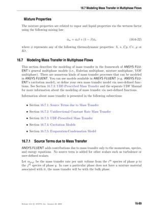
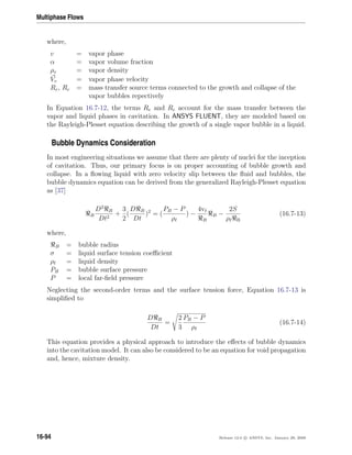
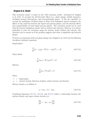
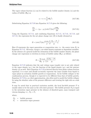
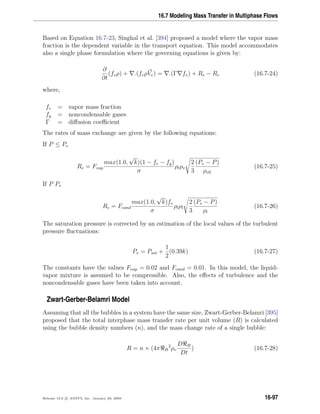
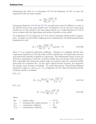
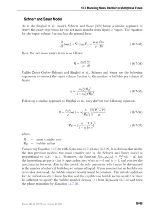
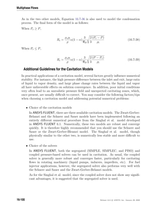
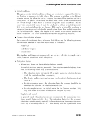
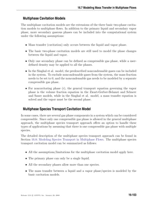
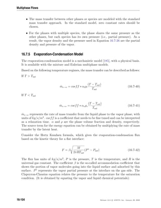
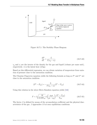
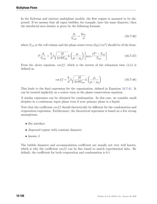
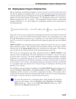
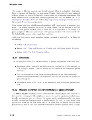
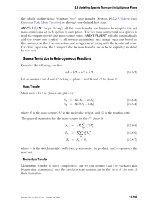
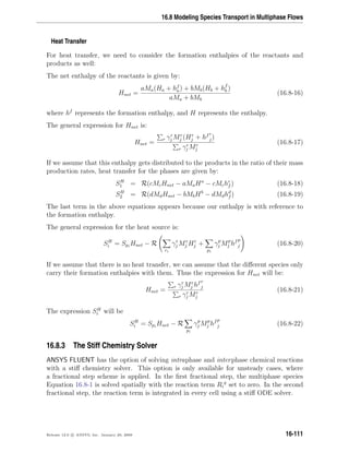

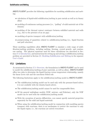
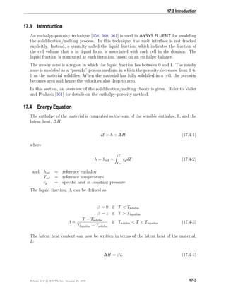
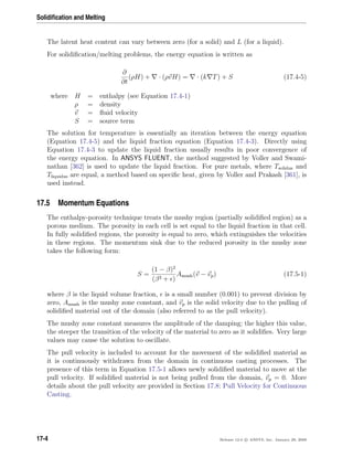
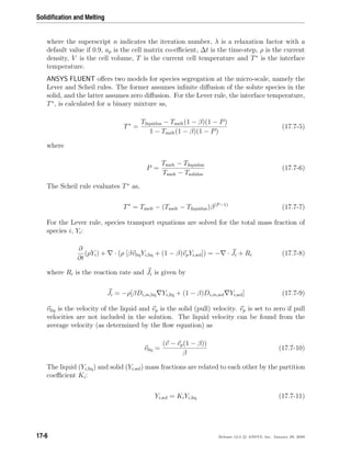
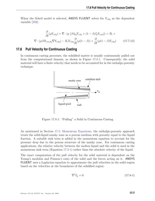

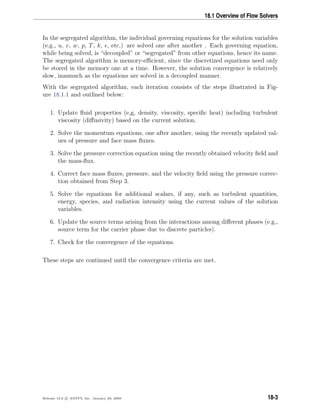
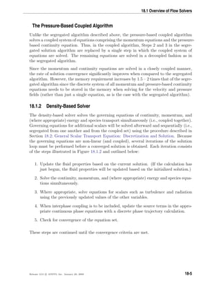
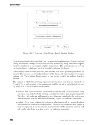
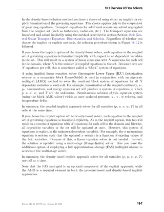
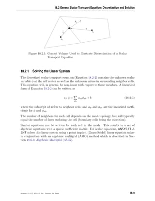
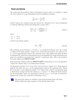
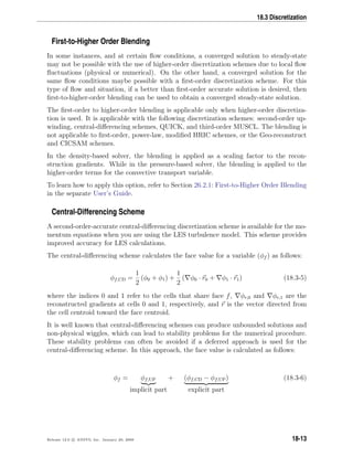
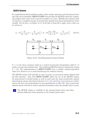
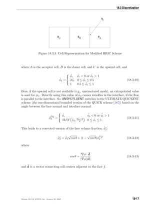
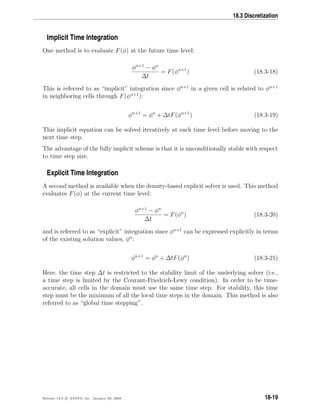
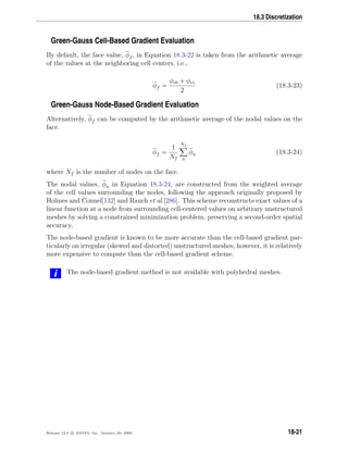
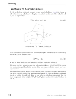
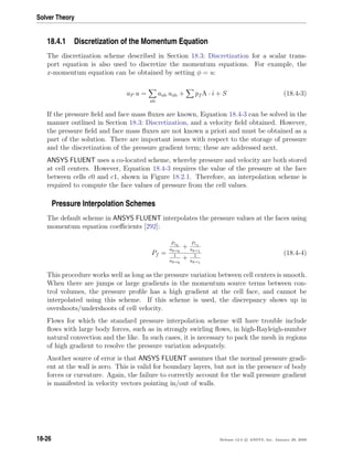
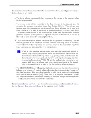
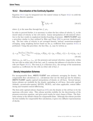
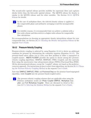
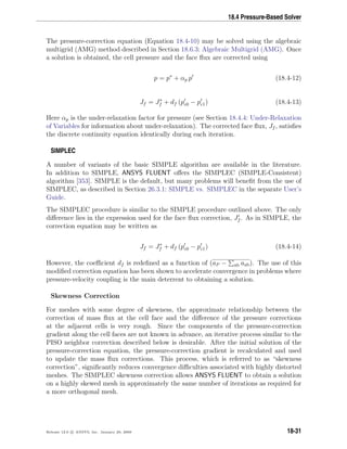
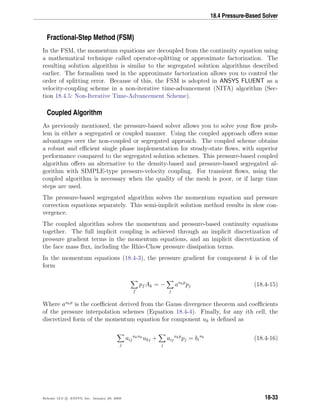
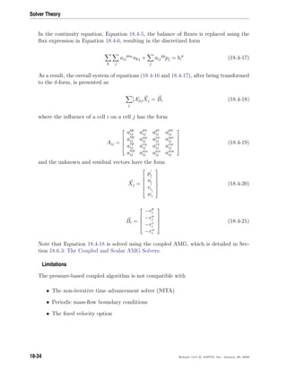
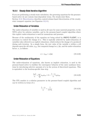
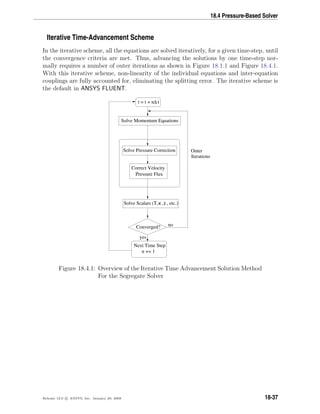
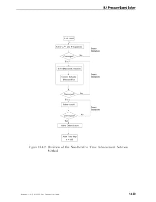
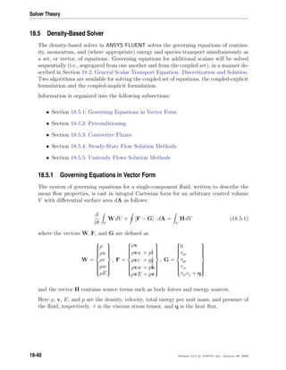
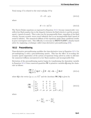
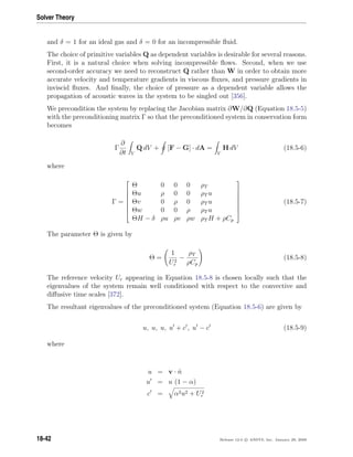
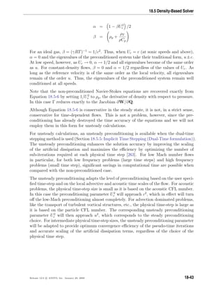
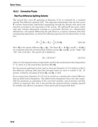
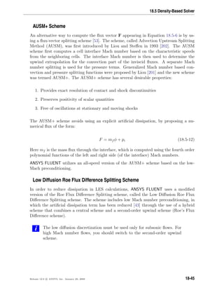
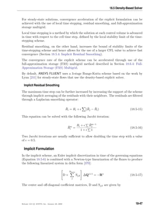
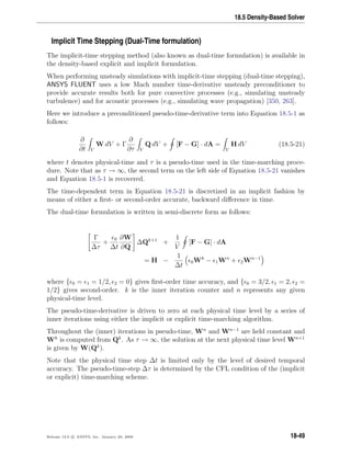
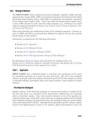
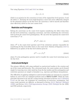
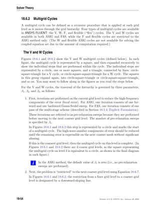
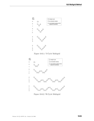
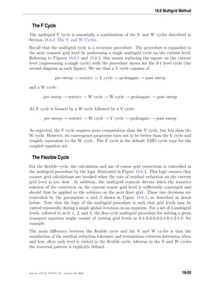
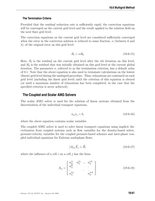
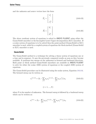
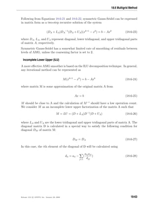
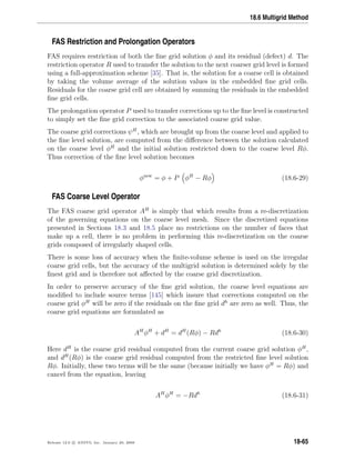
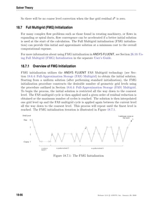
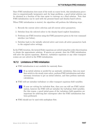

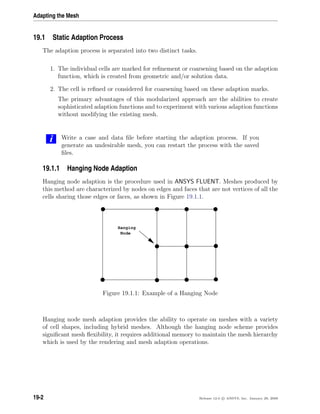
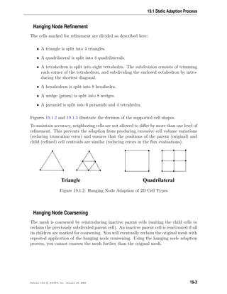

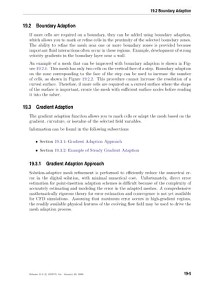
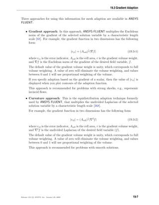
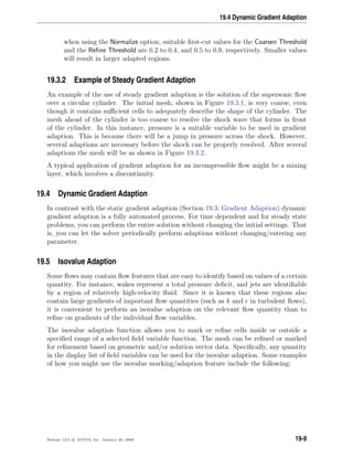
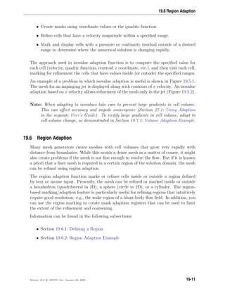
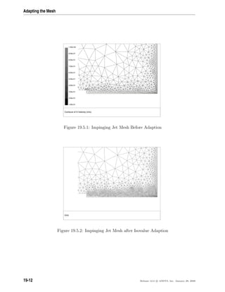
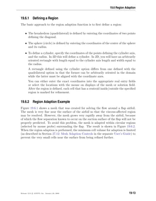
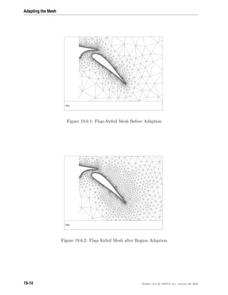
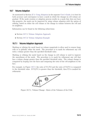
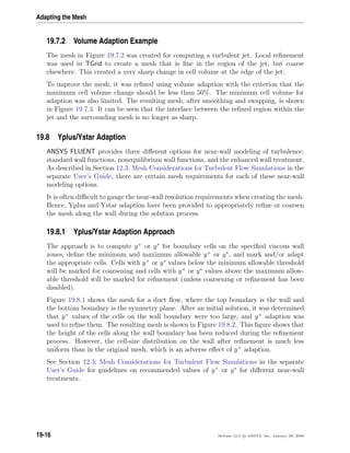
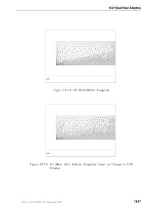
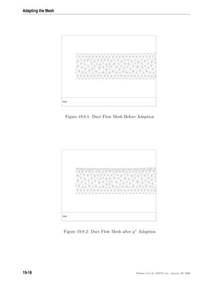
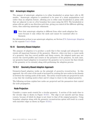
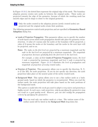
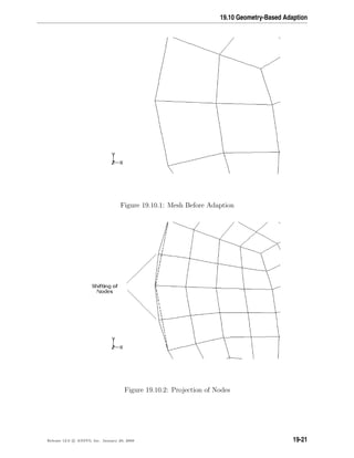
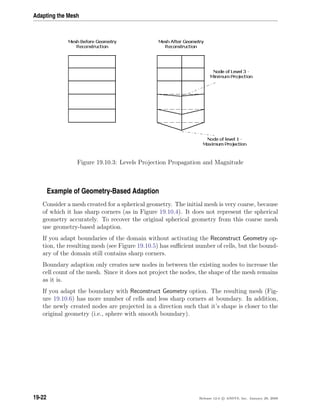

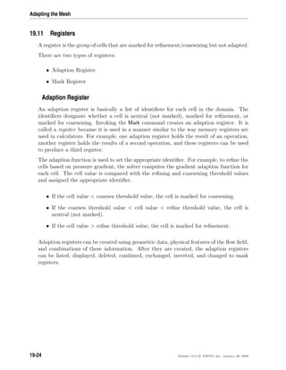
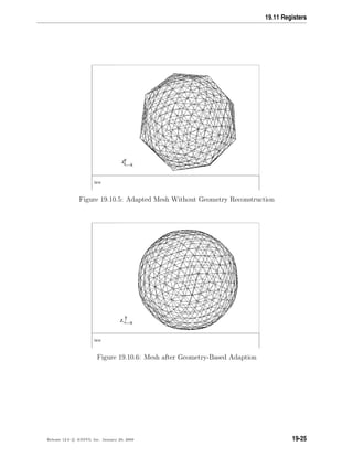
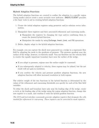
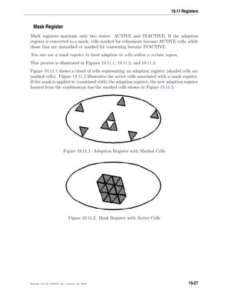
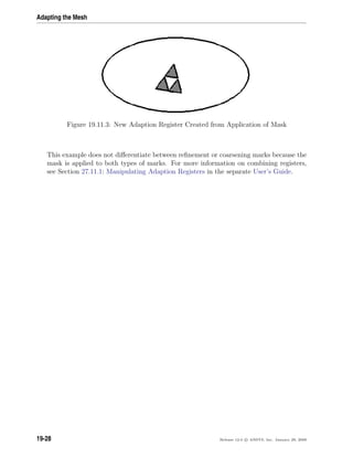
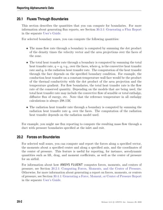
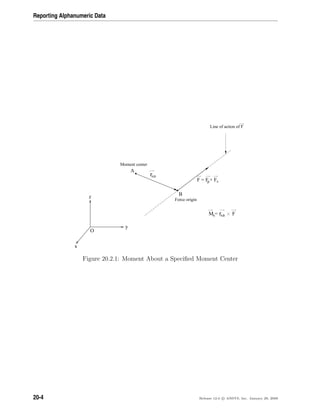
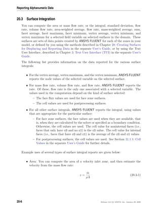
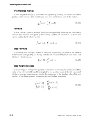
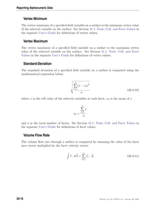
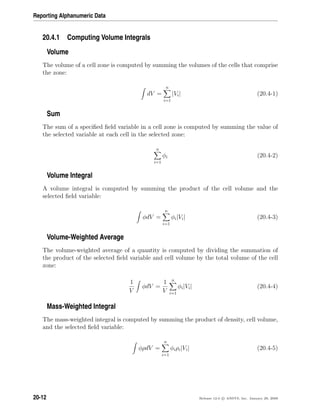


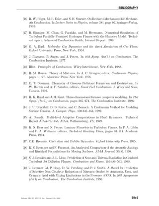
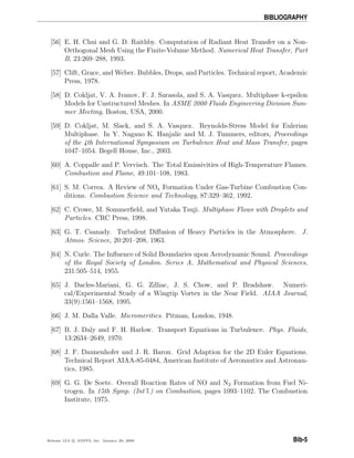

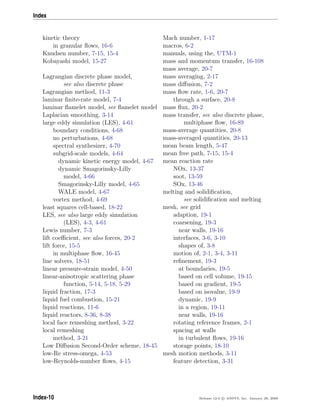
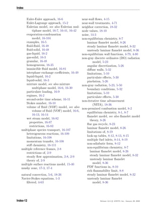
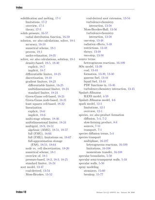

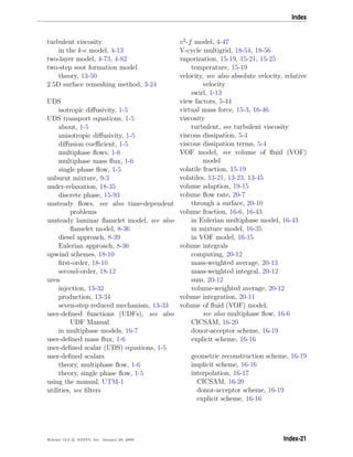

This document is the theory guide for ANSYS FLUENT 12.0. It provides an overview of the physical models available in FLUENT for various fluid flow situations, such as basic fluid flow, flows with rotating reference frames, flows using sliding and deforming meshes, turbulence modeling, heat transfer, and other topics. The guide describes the governing equations and assumptions underlying each model. It is intended to help users understand the theoretical basis of the simulations that can be performed with FLUENT.


