Lecture03

Control-Flow Analysis

Last time
– Undergraduate compilers in a day

Today
– Control-flow analysis
– Building basic blocks
– Building control-flow graphs
– Loops

CIS570 Lecture 3 Control-Flow Analysis 2

Context

Data-flow
– Flow of data values from defs to uses

Control-flow
– Sequencing of operations
e.g., Evaluation of then-code and else-code depends on if-test


1

Representing Control-Flow

High-level representation
– Control flow is implicit in an AST

Low-level representation:
– Use a Control-flow graph (CFG)
– Nodes represent statements (low-level linear IR)
– Edges represent explicit flow of control

Other options
– Control dependences in program dependence graph (PDG) [Ferrante87]
– Dependences on explicit state in value dependence graph (VDG) [Weise 94]


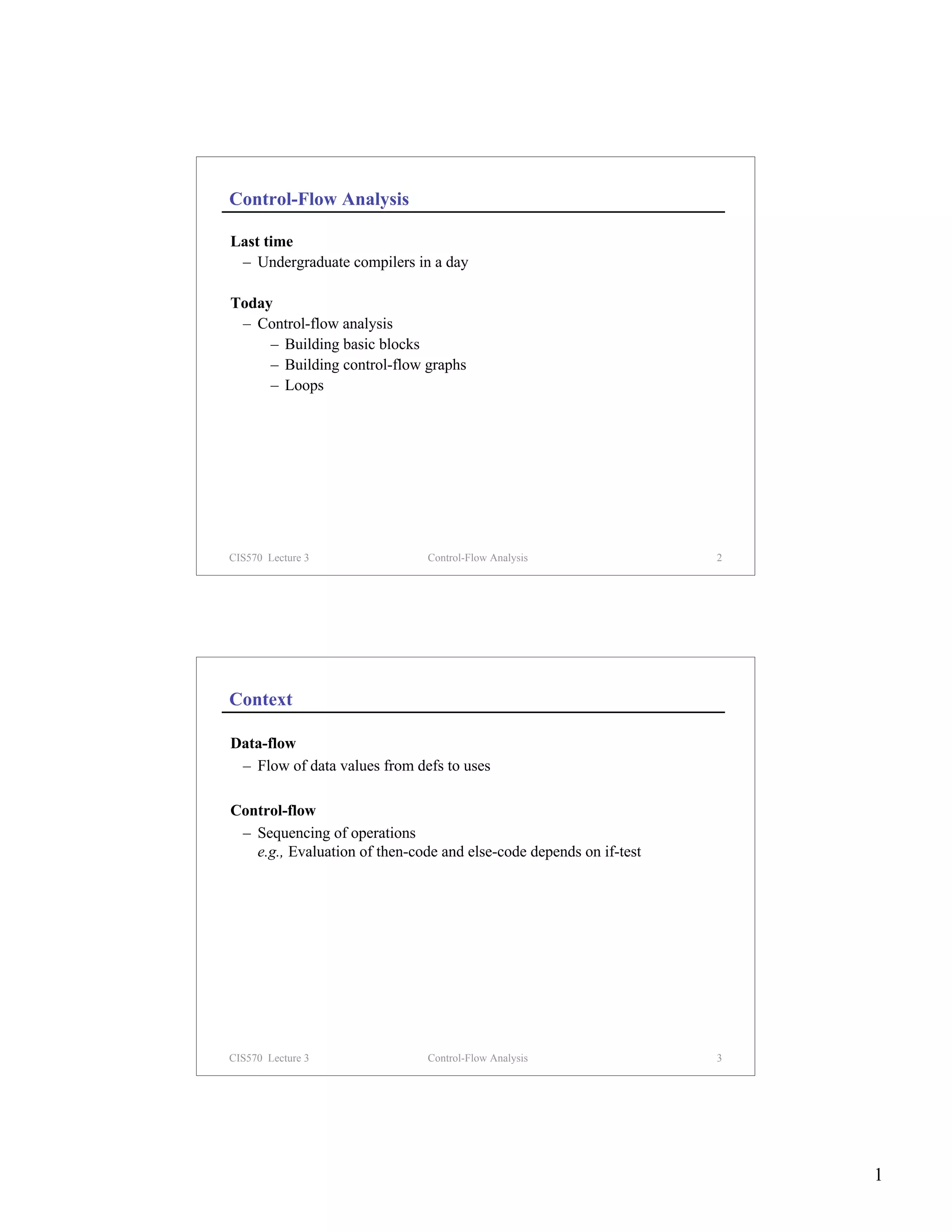
What Is Control-Flow Analysis?

Control-flow analysis discovers the flow of control within a procedure
(e.g., builds a CFG, identifies loops)
1 a := 0
Example b := a * b
1 a := 0
3 c := b/d
2 b := a * b c < x?
3 L1: c := b/d
4 if c < x goto L2 5 e := b / c
5 e := b / c f := e + 1
6 f := e + 1
7 L2: g := f 7 g := f
8 h := t - g h := t - g
9 if e > 0 goto L3 e > 0?
10 goto L1 No Yes
11 L3: return 10 goto 11 return

2

Basic Blocks

Definition
– A basic block is a sequence of straight line code that can be entered only
at the beginning and exited only at the end

g := f
h := t - g
e > 0?
No Yes
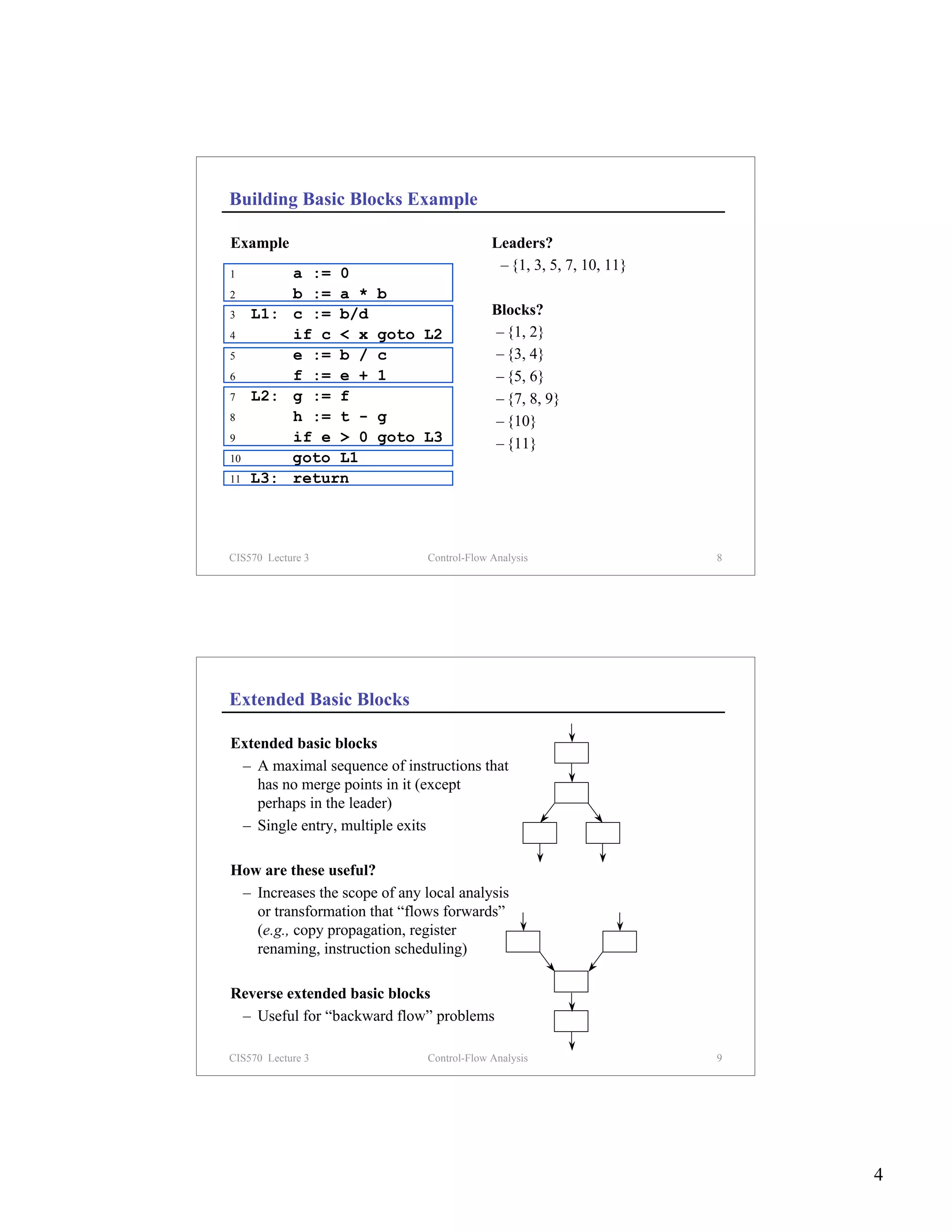
Building basic blocks
– Identify leaders
– The first instruction in a procedure, or
– The target of any branch, or
– An instruction immediately following a branch (implicit target)
– Gobble all subsequent instructions until the next leader


Algorithm for Building Basic Blocks

Input: List of n instructions (instr[i] = ith instruction)
Output: Set of leaders & list of basic blocks
(block[x] is block with leader x)

leaders = {1} // First instruction is a leader
for i = 1 to n // Find all leaders
if instr[i] is a branch
leaders = leaders ∪ set of potential targets of instr[i]
foreach x ∈ leaders
block[x] = { x }
i = x+1 // Fill out x’s basic block
while i ≤ n and i ∉ leaders
block[x] = block[x] ∪ { i }
i=i+1


3

Building Basic Blocks Example

Example Leaders?
1 a := 0 – {1, 3, 5, 7, 10, 11}
2 b := a * b
3 L1: c := b/d Blocks?
4 if c < x goto L2 – {1, 2}
5 e := b / c – {3, 4}
6 f := e + 1 – {5, 6}
7 L2: g := f – {7, 8, 9}
8 h := t - g – {10}
9 if e > 0 goto L3 – {11}
10 goto L1
11 L3: return


Extended Basic Blocks

Extended basic blocks
– A maximal sequence of instructions that
has no merge points in it (except
perhaps in the leader)
– Single entry, multiple exits

How are these useful?
– Increases the scope of any local analysis
or transformation that “flows forwards”
(e.g., copy propagation, register
renaming, instruction scheduling)

Reverse extended basic blocks
– Useful for “backward flow” problems


4

Building a CFG from Basic Blocks

Construction
– Each CFG node represents a basic block
– There is an edge from node i to j if
– Last statement of block i branches to the first statement of j, or
– Block i does not end with an unconditional branch and is
immediately followed in program order by block j (fall through)
Input: A list of m basic blocks (block)
Output: A CFG where each node is a basic block1 1
goto L1:
for i = 1 to m
x = last instruction of block[i] 2

if instr x is a branch L1:
5
for each target (to block j) of instr x
create an edge from block i to block j
if instr x is not an unconditional branch
create an edge from block i to block i+1

Details

Multiple edges between two nodes
...
if (a<b) goto L2
L2: ...
– Combine these edges into one edge

Unreachable code
... – Perform DFS from entry node
goto L1 – Mark each basic block as it is visited
L0: a = 10 – Unmarked blocks are unreachable
L1: ...


5

Challenges

When is CFG construction more challenging?

Languages where jump targets may be unknown
– e.g., Executable code
ld $8, 104($7)
jmp $8

Languages with user-defined control structures
– e.g., Cecil

if ( &{x = 3}, &{a := a + 1}, &{a := a - 1} );


Loop Concepts

Loop: Strongly connected component of CFG
Loop entry edge: Source not in loop & target in loop
Loop exit edge: Source in loop & target not in loop
Loop header node: Target of loop entry edge
Natural loop: Loop with only a single loop header
Back edge: Target is loop header & source is in the loop
Loop tail node: Source of back edge
Loop preheader node: Single node that’s source of the loop entry edge
Nested loop: Loop whose header is inside another loop
Reducible flow graph: CFG whose loops are all natural loops


6

Picturing Loop Terminology

preheader
back edge
entry edge
head

loop
(natural)
tail

exit edge


The Value of Preheader Nodes

Not all loops have preheaders
– Sometimes it is useful to create them h

Without preheader node t
– There can be multiple entry edges
p pre-header
With single preheader node
– There is only one entry edge h

Useful when moving code outside the loop
t
– Don’t have to replicate code for multiple entry
edges


7

Identifying Loops

Why?
– Most execution time spent in loops, so optimizing loops will often give
most benefit

Many approaches
– Interval analysis
– Exploit the natural hierarchical structure of programs
– Decompose the program into nested regions called intervals
– Structural analysis: a generalization of interval analysis
– Identify dominators to discover loops

We’ll look at the dominator-based approach


Dominator Terminology
entry
Dominators
d dom i if all paths from entry to node i include d
d d dom i
Strict dominators
d sdom i if d dom i and d ≠ i entry
i
Immediate dominators
a idom b if a sdom b and there does not exist a node c a idom b a
such that c ≠ a, c ≠ b, a dom c, and c dom b
not ∃ c, a sdom c and c sdom b
b
Post dominators
i
p pdom i if every possible path from i to exit includes
p (p dom i in the flow graph whose arcs are reversed
and entry and exit are interchanged)
p p pdom i

exit

8

Identifying Natural Loops with Dominators
Back edges t
A back edge of a natural loop is one whose target back edge
dominates its source
s
Natural loop
The natural loop of a back edge (m→n), where n n
dominates m, is the set of nodes x such that n natural
dominates x and there is a path from x to m not loop
containing n m
a
a The target, c, of the b
Example
edge (d→c) does not
This loop has two b c
dominate its source, d,
entry points, so (d→c) does not
c and d c d d
define a natural loop
e e

Computing Dominators

Input: Set of nodes N (in CFG) and an entry node s
Output: Dom[i] = set of all nodes that dominate node i

Dom(s) = {s} Key Idea
for each n ∈ N – {s} If a node dominates all
Dom[n] = N predecessors of node n, then it
repeat also dominates node n
change = false
for each n ∈ N – {s} p1 p2 p3 pred[n]
D = {n} ∪ (∩p∈pred(n) Dom[p])
if D ≠ Dom[n] n
change = true
Dom[n] = D
until !change x ∈ Dom(p ) ^ x ∈ Dom(p ) ^ x ∈ Dom(p ) ⇒ x ∈ Dom(n)
1 2 3


9

Computing Dominators (example)

Input: Set of nodes N and an entry node s
Output: Dom[i] = set of all nodes that dominate node i s {s}

Dom(s) = {s} {n, p, q, r, s} q r {n, p, q, r, s}
for each n ∈ N – {s}
p {n, p, q, r, s}
Dom[n] = N
repeat n {n, p, q, r, s}
change = false Initially
for each n ∈ N – {s} Dom[s] = {s}
D = {n} ∪ (∩p∈pred(n) Dom[p]) Dom[q] = {n, p, q, r, s}. . .
if D ≠ Dom[n] Finally
change = true Dom[q] = {q, s}
Dom[n] = D Dom[r] = {r, s}
until !change Dom[p] = {p, s}
Dom[n] = {n, p, s}

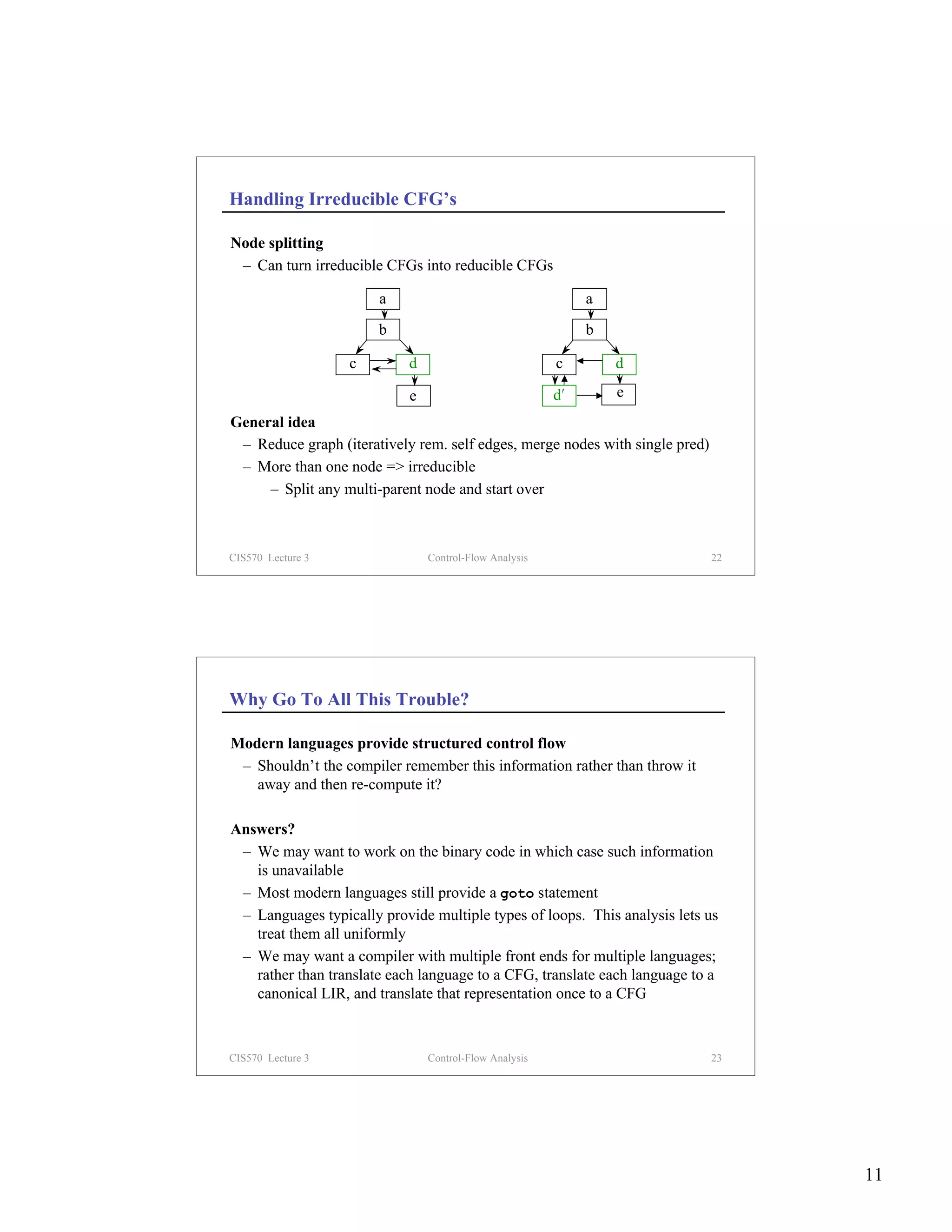
Reducibility

Definition
– A CFG is reducible (well-structured) if we can partition its edges into
two disjoint sets, the forward edges and the back edges, such that
– The forward edges form an acyclic graph in which every node can be
reached from the entry node
– The back edges consist only of edges whose targets dominate their
sources
– Non-natural loops ⇔ irreducibility
Structured control-flow constructs give rise to reducible CFGs
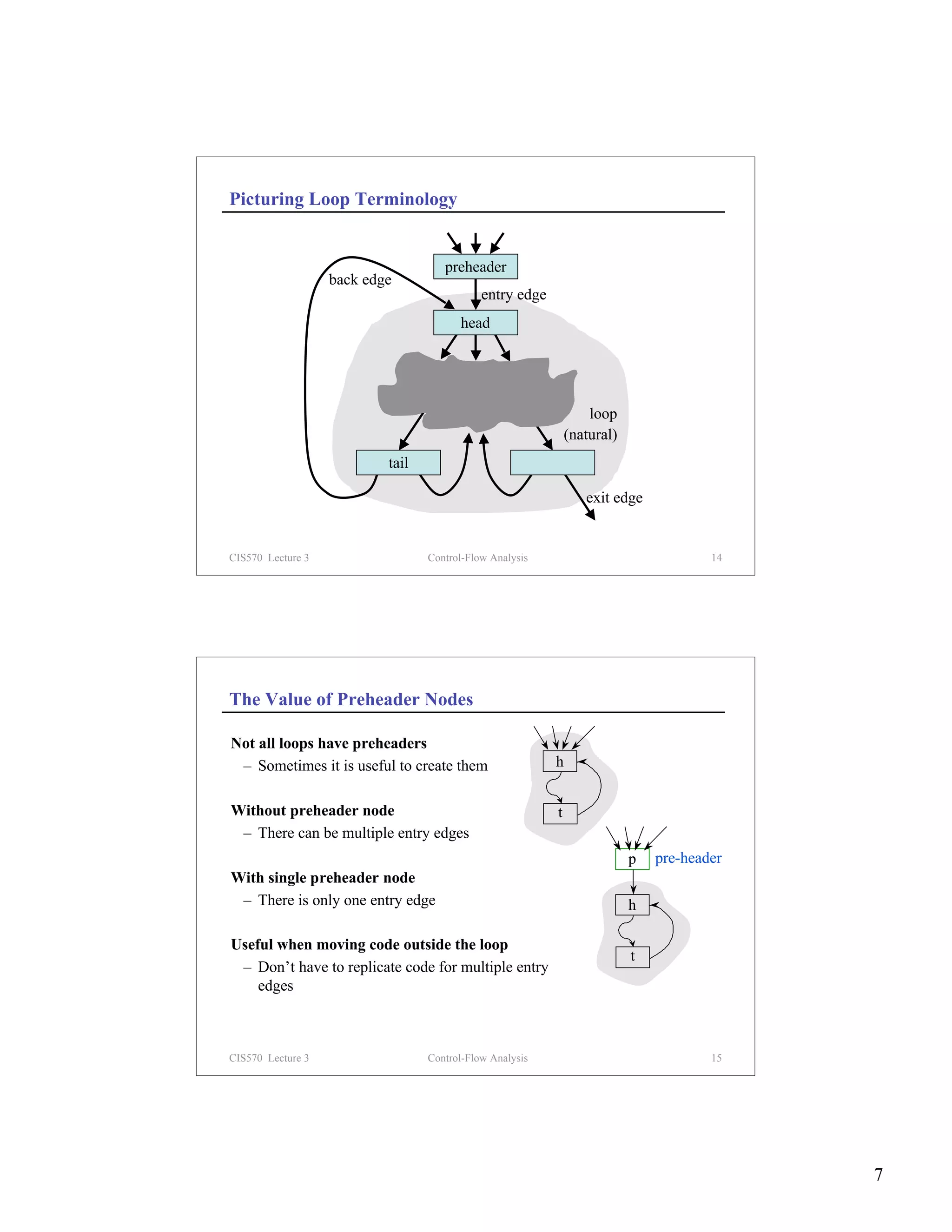
Value of reducibility
– Dominance useful in identifying loops
– Simplifies code transformations (every loop has a single header)
– Permits interval analysis


10

Handling Irreducible CFG’s

Node splitting
– Can turn irreducible CFGs into reducible CFGs

a a
b b

c d c d

e d′ e
General idea
– Reduce graph (iteratively rem. self edges, merge nodes with single pred)
– More than one node => irreducible
– Split any multi-parent node and start over


Why Go To All This Trouble?

Modern languages provide structured control flow
– Shouldn’t the compiler remember this information rather than throw it
away and then re-compute it?

Answers?
– We may want to work on the binary code in which case such information
is unavailable
– Most modern languages still provide a goto statement
– Languages typically provide multiple types of loops. This analysis lets us
treat them all uniformly
– We may want a compiler with multiple front ends for multiple languages;
rather than translate each language to a CFG, translate each language to a
canonical LIR, and translate that representation once to a CFG


11

Concepts

Control-flow analysis
Basic blocks
– Computing basic blocks
– Extended basic blocks
Control-flow graph (CFG)
Loop terminology
Identifying loops
Dominators
Reducibility


Next Time

Discussion
– “Binary Translation” by Sites et al.
– Discussion questions online
– Come prepared

After that: lecture
– Introduction to data-flow analysis


12

Lecture03

More Related Content

What's hot

Viewers also liked

Similar to Lecture03

More from sean chen

Recently uploaded

Lecture03