Download to read offline


![Terminology
Flow Graph Terms
– A CFG node has out-edges that lead to successor nodes and in-edges that
come from predecessor nodes
– pred[n] is the set of all predecessors of node n 1 a = 0
succ[n] is the set of all successors of node n
2 b = a + 1
Examples
– Out-edges of node 5: (5→6) and (5→2) 3 c = c + b
– succ[5] = {2,6}
– pred[5] = {4} 4 a = b * 2
– pred[2] = {1,5}
5 a<9
No Yes
6 return c
CIS570 Lecture 4 Introduction to Data-flow Analysis 8
Uses and Defs
Def (or definition) a = 0
– An assignment of a value to a variable
– def[v] = set of CFG nodes that define variable v
– def[n] = set of variables that are defined at node n
a < 9?
Use
– A read of a variable’s value
v live
– use[v] = set of CFG nodes that use variable v
– use[n] = set of variables that are used at node n
∉ def[v]
More precise definition of liveness
– A variable v is live on a CFG edge if ∈ use[v]
(1) ∃ a directed path from that edge to a use of v (node in use[v]), and
(2) that path does not go through any def of v (no nodes in def[v])
CIS570 Lecture 4 Introduction to Data-flow Analysis 9
4](https://image.slidesharecdn.com/lecture04-110824015452-phpapp01/75/Lecture04-4-2048.jpg)
![Computing Liveness
Rules for computing liveness
(1) Generate liveness: live-in
If a variable is in use[n], n use
it is live-in at node n
(2) Push liveness across edges: pred[n]
live-out live-out live-out
If a variable is live-in at a node n
then it is live-out at all nodes in pred[n] n live-in
(3) Push liveness across nodes:
If a variable is live-out at node n and not in def[n] live-in
n
then the variable is also live-in at n live-out
Data-flow equations
(1) in[n] = use[n] ∪ (out[n] – def[n]) (3)
out[n] = ∪ in[s]
(2)
s ∈ succ[n]
CIS570 Lecture 4 Introduction to Data-flow Analysis 12
Solving the Data-flow Equations
Algorithm
for each node n in CFG
in[n] = ∅; out[n] = ∅ initialize solutions
repeat
for each node n in CFG
in’[n] = in[n] save current results
out’[n] = out[n]
in[n] = use[n] ∪ (out[n] – def[n])
solve data-flow equations
out[n] = ∪ in[s]
s ∈ succ[n]
until in’[n]=in[n] and out’[n]=out[n] for all n test for convergence
This is iterative data-flow analysis (for liveness analysis)
CIS570 Lecture 4 Introduction to Data-flow Analysis 13
6](https://image.slidesharecdn.com/lecture04-110824015452-phpapp01/75/Lecture04-6-2048.jpg)
![Example
1st 2nd 3rd 4th 5th 6th 7th
node use def in out in out in out in out in out in out in out
# 1 a := 0
1 a a a ac c ac c ac c ac
2 a b a a bc ac bc ac bc ac bc ac bc ac bc 2 b := a + 1
3 bc c bc bc b bc b bc b bc b bc bc bc bc
4 b a b b a b a b ac bc ac bc ac bc ac 3 c := c + b
5 a a a a ac ac ac ac ac ac ac ac ac ac ac
6 c c c c c c c c 4 a := b * 2
Data-flow Equations for Liveness 5 a < 9?
No Yes
in[n] = use[n] ∪ (out[n] – def[n])
6 return c
out[n] = ∪ in[s]
s ∈ succ[n]
CIS570 Lecture 4 Introduction to Data-flow Analysis 14
Example (cont)
Data-flow Equations for Liveness
in[n] = use[n] ∪ (out[n] – def[n]) 1 a := 0
out[n] = ∪ in[s] 2 b := a + 1
s ∈ succ[n]
3 c := c + b
Improving Performance out[3]
Consider the (3→4) edge in the graph: in[4]
4 a := b * 2
out[4]
out[4] is used to compute in[4]
in[4] is used to compute out[3] . . . 5 a < 9?
So we should compute the sets in the No Yes
order: out[4], in[4], out[3], in[3], . . . 6 return c
The order of computation should follow the direction of flow
CIS570 Lecture 4 Introduction to Data-flow Analysis 15
7](https://image.slidesharecdn.com/lecture04-110824015452-phpapp01/75/Lecture04-7-2048.jpg)
![Iterating Through the Flow Graph Backwards
1st 2nd 3rd
node use def out in out in out in 1 a := 0
#
6 c c c c
2 b := a + 1
5 a c ac ac ac ac ac
4 b a ac bc ac bc ac bc 3 c := c + b
3 bc c bc bc bc bc bc bc
2 a b bc ac bc ac bc ac 4 a := b * 2
1 a ac c ac c ac c
5 a < 9?
Converges much faster!
No Yes
6 return c
CIS570 Lecture 4 Introduction to Data-flow Analysis 16
Solving the Data-flow Equations (reprise)
Algorithm
for each node n in CFG
in[n] = ∅; out[n] = ∅ Initialize solutions
repeat
for each node n in CFG in reverse topsort order
in’[n] = in[n] Save current results
out’[n] = out[n]
out[n] = s ∈ succ[n] in[s]
∪
Solve data-flow equations
in[n] = use[n] ∪ (out[n] – def[n])
until in’[n]=in[n] and out’[n]=out[n] for all n Test for convergence
CIS570 Lecture 4 Introduction to Data-flow Analysis 17
8](https://image.slidesharecdn.com/lecture04-110824015452-phpapp01/75/Lecture04-8-2048.jpg)
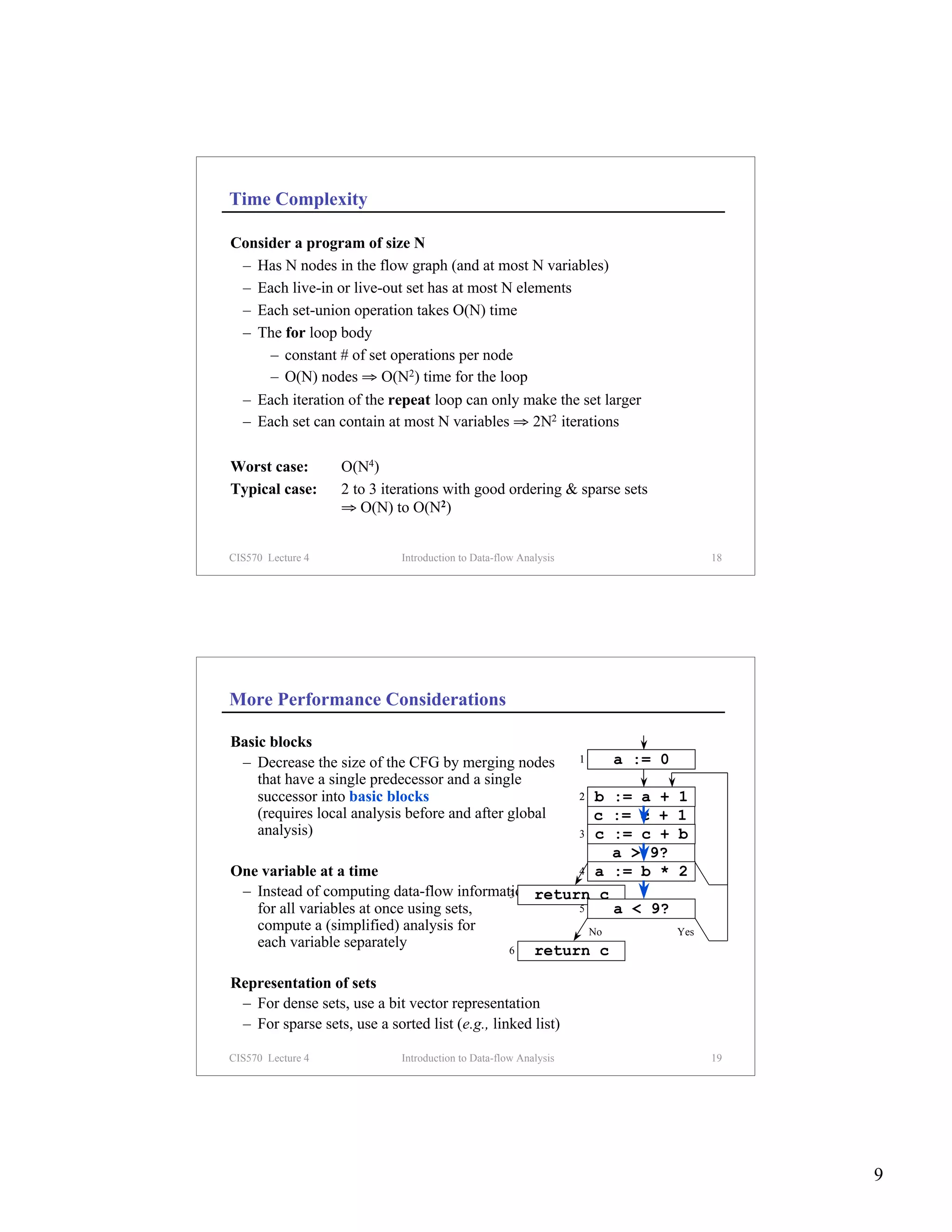
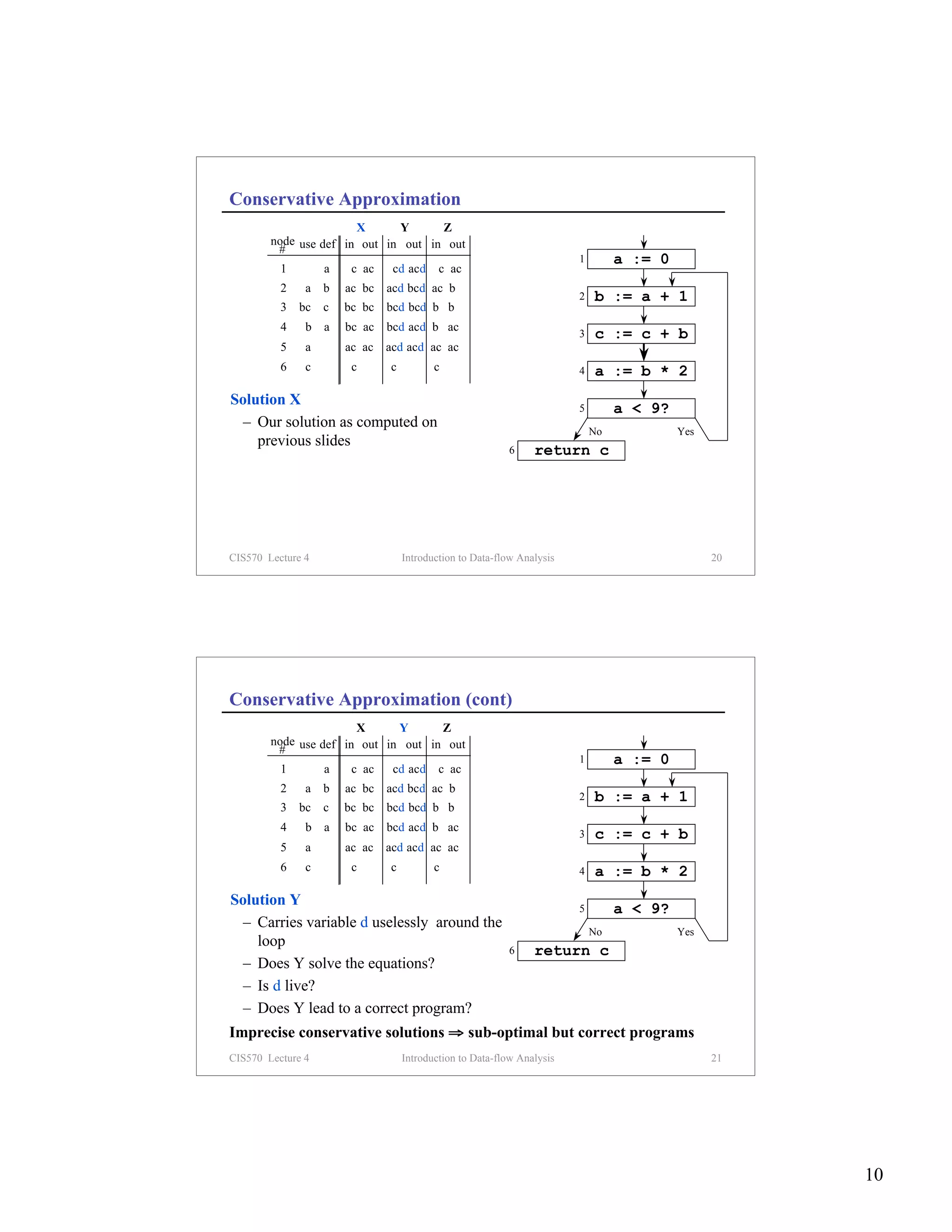
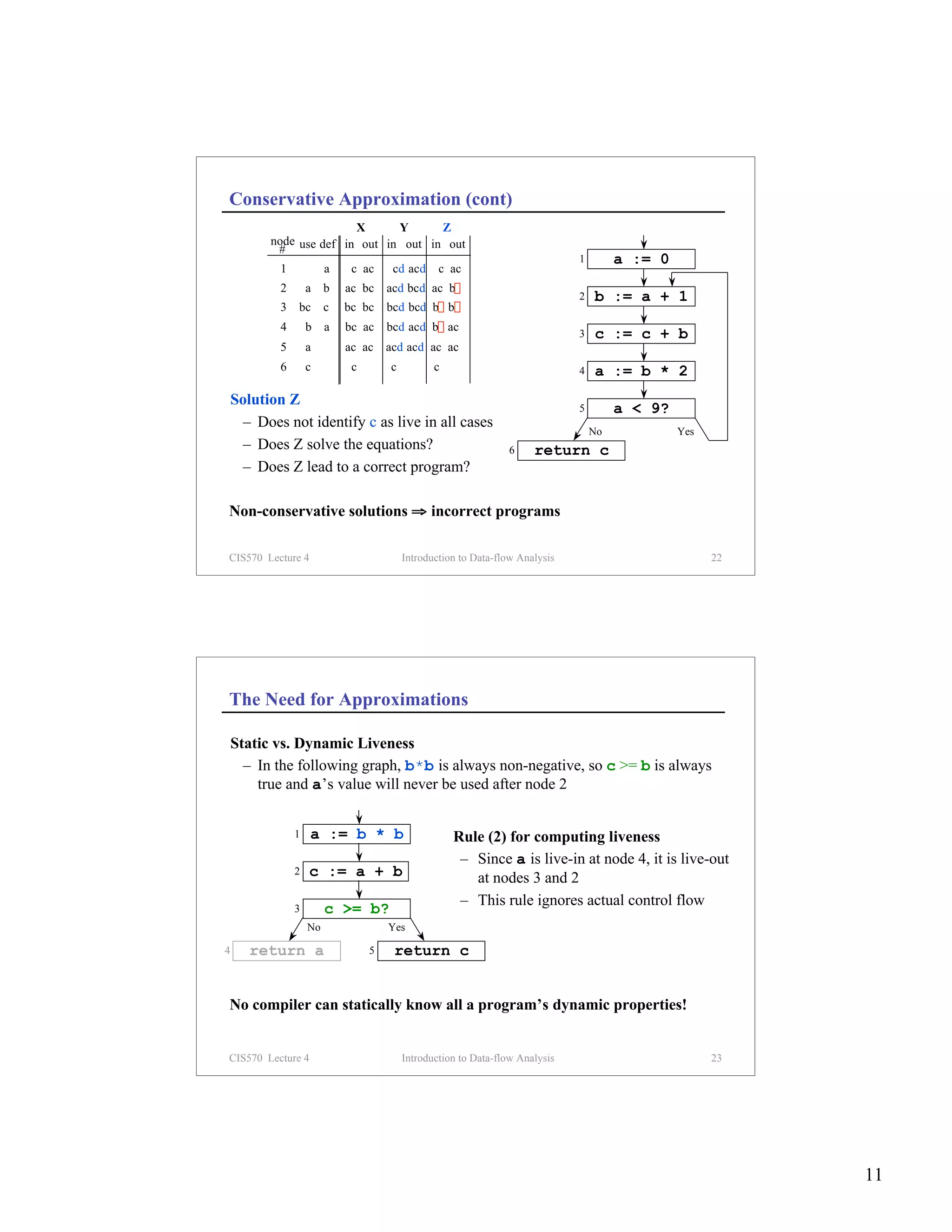

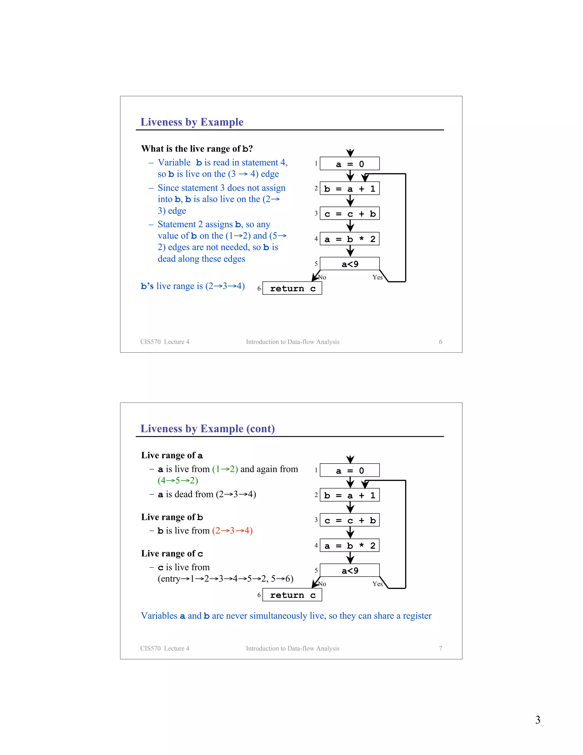
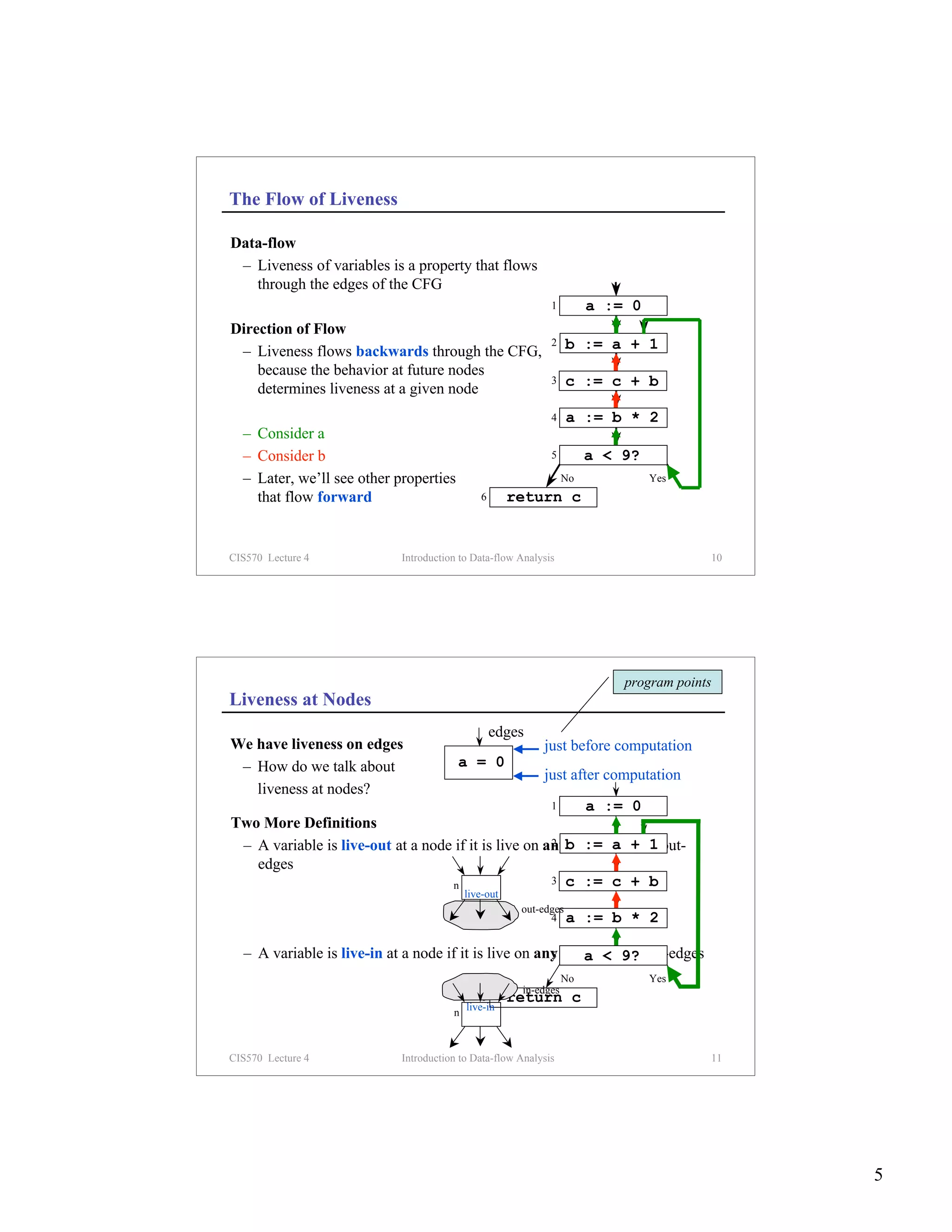
The document introduces data-flow analysis, which derives information about a program's dynamic behavior by examining its static code. It discusses liveness analysis, which determines whether a variable is live (will be used in the future) or dead at a given point. The concepts of control flow graphs, uses/defs, and solving the data-flow equations through iterative analysis are explained. An example liveness analysis is worked through to demonstrate the process.