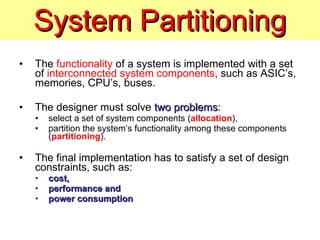
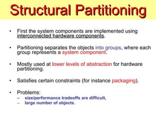
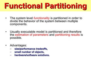
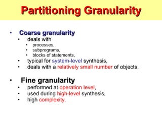
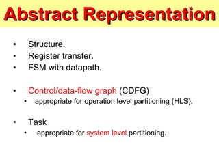
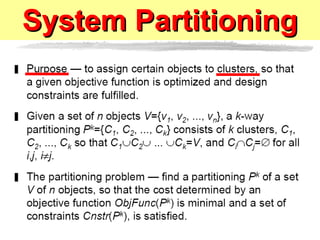
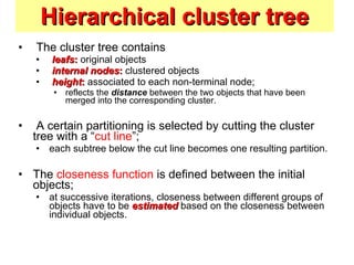
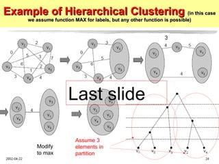
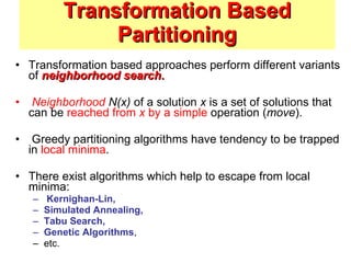
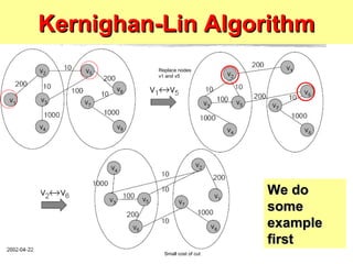
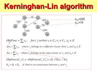
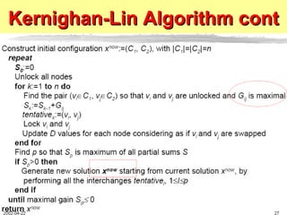
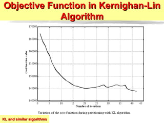
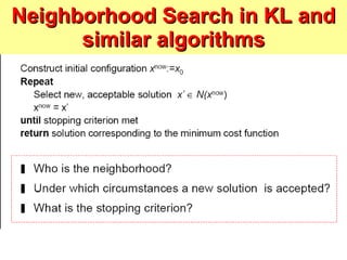
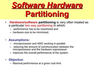
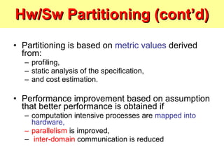
The document discusses system partitioning for designing interconnected hardware components. It describes different types of partitioning including structural, functional, and granularity partitioning. Automatic partitioning approaches include constructive clustering and iterative transformation-based methods. Hierarchical clustering is a constructive approach that groups objects into partitions based on closeness metrics. Transformation-based methods perform neighborhood searches using algorithms like Kernighan-Lin and simulated annealing to optimize an objective function. Hardware-software partitioning aims to maximize performance by mapping computation-intensive processes to hardware while minimizing communication between hardware and software components.

1. System Partitioning Kris Kuchcinski [email_address]

2. Partitioning “ He who can properly define and divide is to be considered a god.” Plato (ca 429-347 BC)

3. System Partitioning The functionality of a system is implemented with a set of interconnected system components , such as ASIC’s, memories, CPU’s, buses. The designer must solve two problems : select a set of system components ( allocation ), partition the system’s functionality among these components ( partitioning ). The final implementation has to satisfy a set of design constraints, such as: cost, performance and power consumption

4. Structural Partitioning First the system components are implemented using interconnected hardware components . Partitioning separates the objects into groups , where each group represents a system component . Mostly used at lower levels of abstraction for hardware partitioning. Satisfies certain constraints (for instance packaging ). Problems: size/performance tradeoffs are difficult, large number of objects .

5. Functional Partitioning The system level functionality is partitioned in order to divide the behavior of the system between multiple components. Usually executable model is partitioned and therefore the estimation of parameters and partitioning results is possible. Advantages: size/performance tradeoffs, small number of objects, hardware/software solutions.

6. Partitioning Granularity Coarse granularity deals with processes, subprograms, blocks of statements, typical for system-level synthesis, deals with a relatively small number of objects. Fine granularity performed at operation level , used during high-level synthesis, high complexity.

7. Abstract Representation Structure. Register transfer. FSM with datapath. Control/data-flow graph (CDFG) appropriate for operation level partitioning (HLS). Task appropriate for system level partitioning.

8. Task Partitioning

9. CDFG Partitioning

10. System Partitioning

11. Metrics and Estimations ❚ Partitioning algorithms have to rely on a quantitative measure of a candidate solution’s goodness. ❚ Metrics — attributes which characterize a given solution; they are expressed quantitatively. ❚ Metrics include: cost, execution time, communication rates, power consumption, testability, reliability, program size, data size and memory size.

12. Metrics and Estimations Estimation determines a metric value from a rough implementation . Inaccuracy can be tolerated as long as the relative goodness of any two partitions is determined correctly.

13. Objective Function and Closeness function Objective function : a combination of metrics which captures the overall quality of a certain partitioning. Closeness function : captures the benefit gained from grouping two objects into the same partition; it is based on a local view of the system.

14. Example Partitioning Objective We want to minimize this function

15. Example of an Objective Function We want to minimize this function

16. Design Constraints We want to minimize this function

17. Example of an Objective Function We want to minimize this function

18. Closeness Function We want to maximize this function

19. Partitioning Approaches Manually guided partitioning Needs strong support from design environment : estimation tools & schedulers, facilities to interactively perform predefined transformations and to define new ones, graphical interfaces . Automatic partitioning

20. Automatic Partitioning The partitioning problem is NP-complete. The design space has to be explored according to a certain strategy This strategy converges towards a solution close to one which yields the minimal cost.

21. Automatic Partitioning Approaches Constructive (clustering) bottom up approach: each object initially belongs to its own cluster, and clusters are then gradually merged until the desired partitioning is found; does not require a global view of the system relies only on local relations between objects ( closeness metrics).

22. Automatic Partitioning Approaches (cont’d) Iterative (transformation-based) based on a design space exploration which is guided by an objective function that reflects the global quality of the partitioning; a starting solution is modified iteratively , by passing from one candidate solution to another passing is based on evaluations of an objective function.

23. Hierarchical clustering A constructive approach: performed in several iterations with final goal to group a set of objects into partitions according to some measure of closeness. At each iteration the two closest objects are grouped together; the process is iterated until a single cluster is produced.

24. Hierarchical cluster tree The cluster tree contains leafs : original objects internal nodes : clustered objects height : associated to each non-terminal node; reflects the distance between the two objects that have been merged into the corresponding cluster. A certain partitioning is selected by cutting the cluster tree with a “ cut line ”; each subtree below the cut line becomes one resulting partition. The closeness function is defined between the initial objects; at successive iterations, closeness between different groups of objects have to be estimated based on the closeness between individual objects.

25. Example of Hierarchical Clustering (in this case we assume function MAX for labels, but any other function is possible) Modify to max Assume 3 elements in partition Last slide 3

26. Transformation Based Partitioning Transformation based approaches perform different variants of neighborhood search . Neighborhood N(x) of a solution x is a set of solutions that can be reached from x by a simple operation ( move ). Greedy partitioning algorithms have tendency to be trapped in local minima . There exist algorithms which help to escape from local minima: Kernighan-Lin, Simulated Annealing, Tabu Search, Genetic Algorithms , etc.

27. Kernighan-Lin Algorithm Replace nodes v1 and v5 Small cost of cut We do some example first

28. Kerninghan-Lin algorithm

29. Kernighan-Lin Algorithm cont

30. Objective Function in Kernighan-Lin Algorithm KL and similar algorithms

31. Neighborhood Search in KL and similar algorithms

32. Simulated Annealing for generating X now

33. Simulated Annealing may worsen the solution. Best one must be remembered

34. Software Hardware Partitioning Hardware/software partitioning is very often treated as a particular two way partitioning in which: performance has to be maximized and hardware size to be minimized; Assumptions : microprocessor and ASIC working in parallel; reducing the amount of communication between the microprocessor and the hardware coprocessor improves the overall performance of the system. Objective : Maximal performance at a given cost limit.

35. Hw/Sw Partitioning (cont’d) Partitioning is based on metric values derived from: profiling, static analysis of the specification, and cost estimation. Performance improvement based on assumption that better performance is obtained if computation intensive processes are mapped into hardware, parallelism is improved, inter-domain communication is reduced

36. Summary on paritioning in System level synthesis The partitioning problem is NP-complete and has to be solved using optimization heuristics. Partitioning heuristics are constructive or transformation based. Hierarchical clustering is one of the most used constructive approaches. Transformational approaches are based on neighborhood search. A hardware software partitioning for acceleration is done by placing computation intensive processes into hardware, improving parallelism and reducing inter-domain communication.

37. Literature P. Eles, K. Kuchcinski and Z. Peng, System Synthesis with VHDL , Kluwer Academic Publisher, 1998.