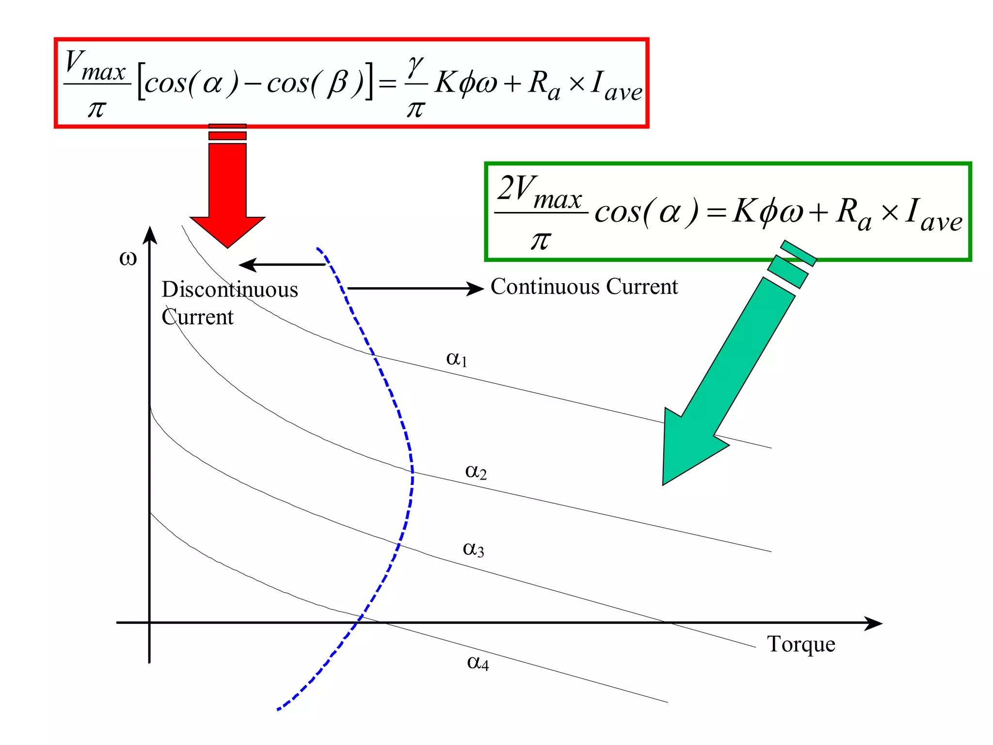
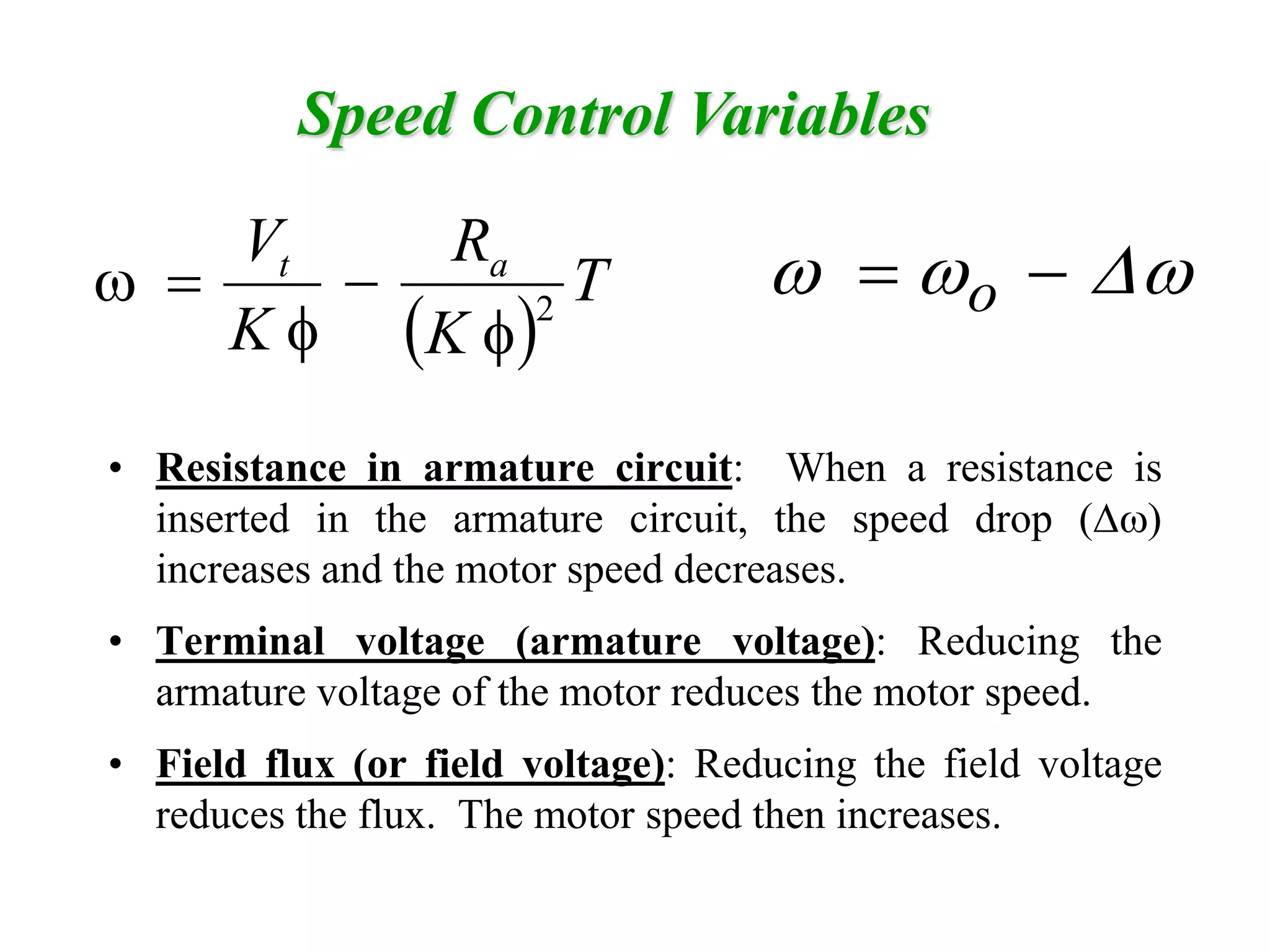
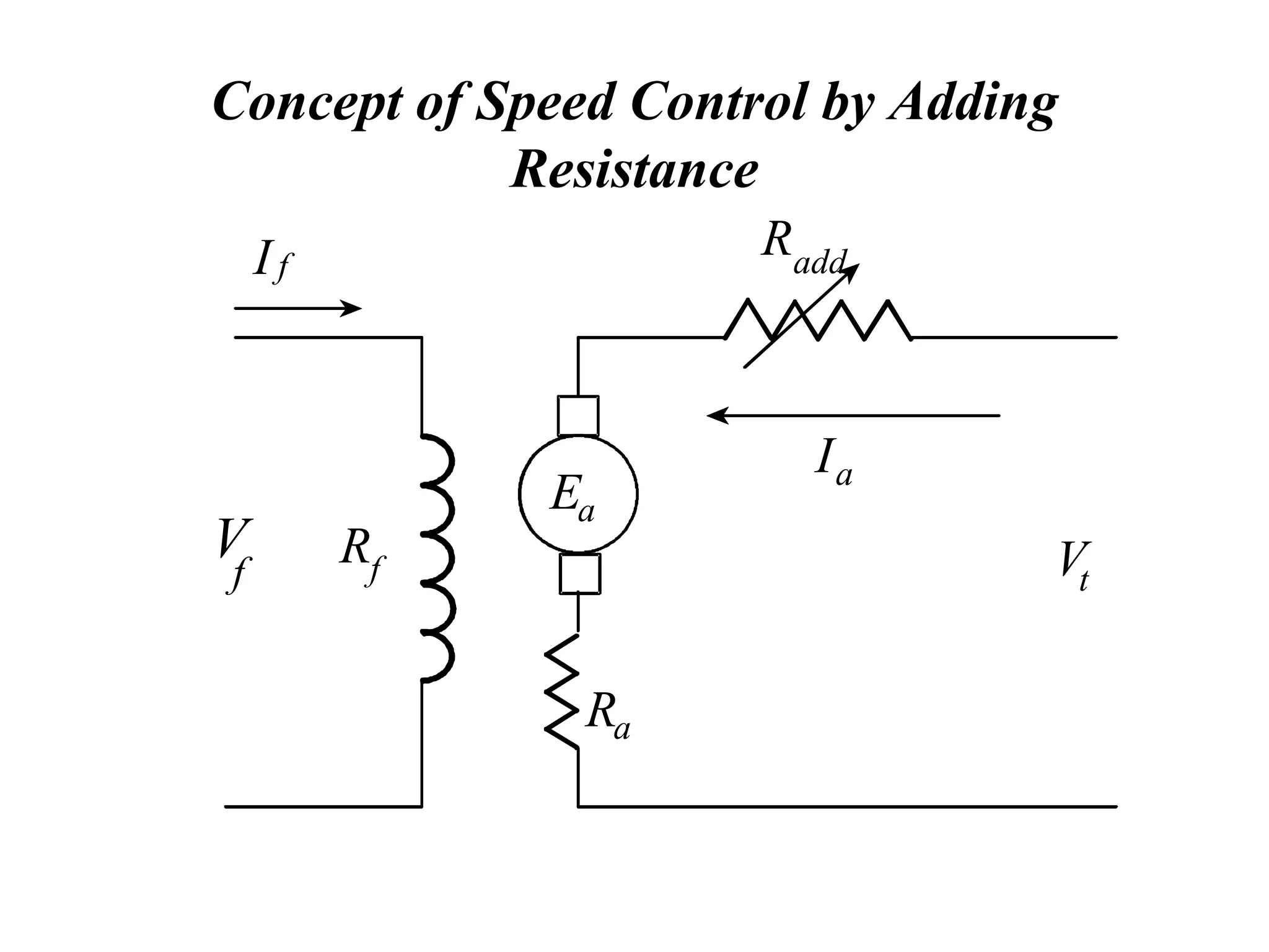
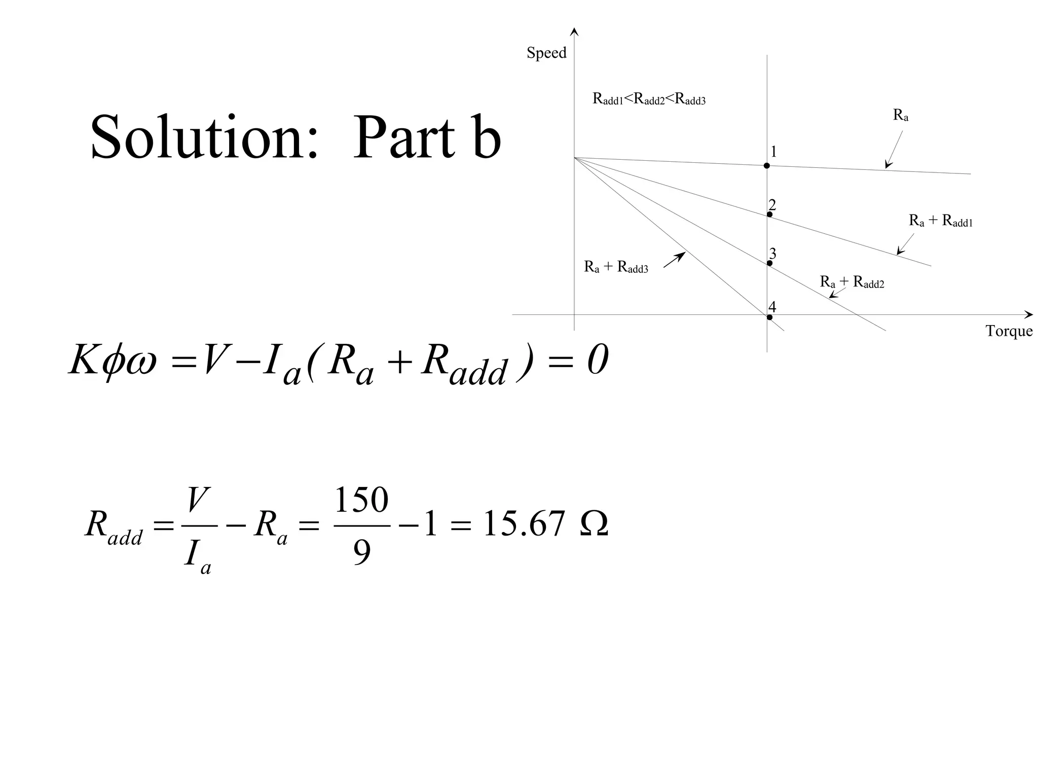
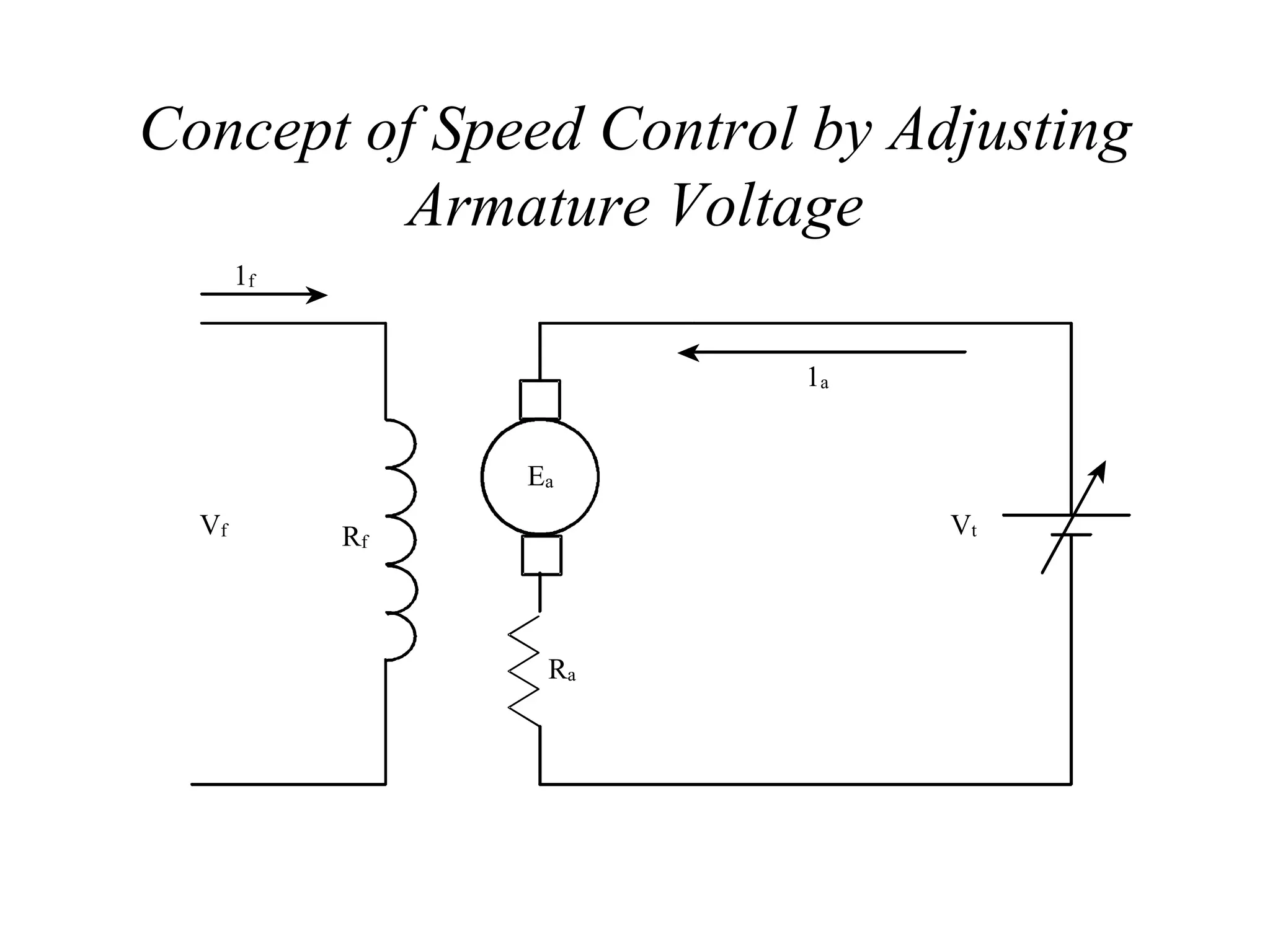
This document discusses speed control of DC motors. It provides three main methods for controlling motor speed: 1) adding resistance to the armature circuit which decreases motor speed, 2) reducing the armature voltage which also decreases speed, and 3) reducing the field voltage which increases motor speed. It also discusses attributes of good speed controllers and concepts like adding variable resistance or adjusting field/armature voltage to achieve speed control. Examples are provided to demonstrate calculating motor speed under different load or resistance conditions.

1. Chapter 6: Speed Control of Direct
Current Motors

2.  
T
K
R
K
V a
t
2





• Resistance in armature circuit: When a resistance is
inserted in the armature circuit, the speed drop (D)
increases and the motor speed decreases.
• Terminal voltage (armature voltage): Reducing the
armature voltage of the motor reduces the motor speed.
• Field flux (or field voltage): Reducing the field voltage
reduces the flux. The motor speed then increases.

D

 
 o
Speed Control Variables

3. Attributes of good speed controller
• Soft transition
• Sufficient speed damping
• Over-voltage must not exceed the tolerable limit
of the system components.
• The magnitude of the inrush current should be
kept under control
• Natural electromechanical oscillations should be
avoided.

4. Concept of Speed Control by Adding
Resistance
V
f
If
Ia
Radd
Rf
Ra
Ea
Vt

5. 2
o
2
add
a
t
2 T
)
K
(
R
R
K
V

D



 




Speed
Torque
Ra
Radd1<Radd2<Radd3
1
Ra + Radd1
2
Ra + Radd2
3
Ra + Radd3
4
1
2
1
)
(

D







 o
a
t
T
K
R
K
V
o


6. Example 6.1
A 150 V, dc shunt motor drives a constant-torque
load at a speed of 1200 rev/min. The armature and
field resistances are 1 W and 150 W respectively.
The motor draws a line current of 10 A at the given
load.
a. Calculate the resistance that should be added to the
armature circuit to reduce the speed by 50%.
b. Calculate the resistance that must be added to the
armature circuit to operate the motor at holding
condition.

7. Solution: Part a
A
I
I
I f
a 9
150
150
10
1
1 




)
R
R
(
I
V
K
E
R
I
V
K
E
1
add
a
2
a
2
2
a
a
1
a
1
1
a












K
T
I d
a  2
a
1
a I
I 
)
R
R
(
I
V
R
I
V
n
n
E
E
1
add
a
a
a
a
2
1
2
1
2
a
1
a








)
R
1
(
9
150
1
9
150
1200
5
.
0
1200
1
add







W
 83
.
7
1
add
R
Speed
Torque
Ra
Ra + Radd1
Ra + Radd2
Ra + Radd3
Radd1<Radd2<Radd3
1
2
3
4
Ra
I
If Rf Vt
Ea
Ia

8. Solution: Part b
0
)
R
R
(
I
V
K add
a
a 





W




 67
.
15
1
9
150
a
a
add R
I
V
R
Speed
Torque
Ra
Ra + Radd1
Ra + Radd2
Ra + Radd3
Radd1<Radd2<Radd3
1
2
3
4

9. Concept of Speed Control by Adjusting
Armature Voltage
1f
1a
Vf Rf
Ea
Ra
Vt

10. T
)
K
(
R
K
V
2
a
t


 

V1
Ttot
Torque
1
o1
V2
2
o2
V3
3
o3
V4
4
o4
V1>V2>V3>V4


11. Concept of Speed Control by Adjusting
Field Voltage
Vf
If
Ia
Ea
Ra
Rf Vt

12. T
)
K
(
R
K
V
2
a
t


 

o1
Vf1

Ttot
Torque
Vf1>Vf2>Vf3
o2
Vf2
2
1
o3 Vf3
3

13. Example 6.3
• A 150 V, dc shunt motor drives a constant-
torque load at a speed of 1200 rev/min. The
armature and field resistances are 2 W and
150 W respectively. The motor draws a line
current of 10 A. Assume that a resistance is
added in the field circuit to reduce the field
current by 20%. Calculate the armature
current, motor speed, the value of the added
resistance, and the extra field losses.

14. Solution
Ra
I
If Rf Vt
Ea
Ia
A
I
I
I f
a 9
150
150
10
1
1 





15. Solution
2
a
2
1
a
1
d I
K
I
K
T 
 

1
a
2
1
2
a I
I



A
25
.
11
9
8
.
0
1
I
I
I
I 1
a
2
f
1
f
2
a 


a
2
a
2
2
2
a
a
1
a
1
1
1
a
R
I
V
K
E
R
I
V
K
E










a
2
a
a
1
a
2
1
2
1
R
I
V
R
I
V
n
n





2
25
.
11
150
2
9
150
n
1200
8
.
0
1
2 




rpm
n 86
.
1448
2 
o1
o2 Vf2
Vf1

Td
Torque
Vf1>Vf2
1
2

16. Solid-State Control
Converter
Motor
Rectifier
& Filter
Field

17. VAK
VS
Ra
La
Ea
Vt
Single-Phase, Half-Wave Drives
)]
(
1
[
)
(
)
sin
(
)]
(
1
[
)
(
max 







 u
u
E
u
u
t
V
v
u
u
E
u
u
v
v
a
t
a
s
t











18. )]
(
1
[
)
(
)
sin
(
)]
(
1
[
)
(
max 







 u
u
E
u
u
t
V
v
u
u
E
u
u
v
v
a
t
a
s
t










-200.00
-150.00
-100.00
-50.00
0.00
50.00
100.00
150.00
200.00
0 90 180 270 360 450 540
Angle
vs
i
i
Ea
vt
vt
Ea+i Ra



19.   ave
a
a
a
s
ave
a
a
a
s
ave
a
a
t
t
ave
a
a
t
I
R
E
E
t
d
v
I
R
E
t
d
E
t
d
v
I
R
E
t
d
v
t
d
v
I
R
E
t
d
v



















































 
 
















2
2
1
2
1
2
1
2
1
2
2
2
0
VAK
VS
Ra
La
Ea
Vt
a
L
a
t R
i
v
E
v 


a
ave
ave
L
a
ave
t R
I
V
E
V 


a
ave
a
ave
t R
I
E
V 


20. ave
a
ave
a
a
I
R
K
V
I
R
E
V

















2
]
cos
[cos
2
2
]
cos
[cos
2
max
max
VAK
VS
Ra
La
Ea
Vt


 

 
  ave
a
a
a
s
ave
a
a
a
s
I
R
E
E
t
d
v
I
R
E
E
t
d
v








































2
2
1
2
2
1

21. 


K
I
R
K
V a
a
t










K
I
R
K
V
Then
V
V
and
K
K
Let
a
a
t
t
~
~
~
]
cos
[cos
2
~
2
~
max





ave
a I
R
K
V








 2
]
cos
[cos
2
max

22. Example 6.3
• A 1-hp dc shunt motor is loaded by a
constant torque of 10 NM. The
armature resistance of the motor is 5 W,
and the field constant K = 2.5 V sec.
The motor is driven by a half wave SCR
converter. The power source is 120 V,
60 Hz. The triggering angle of the
converter is 60o, and the conduction
period is 150o. Calculate the motor
speed and the developed power.

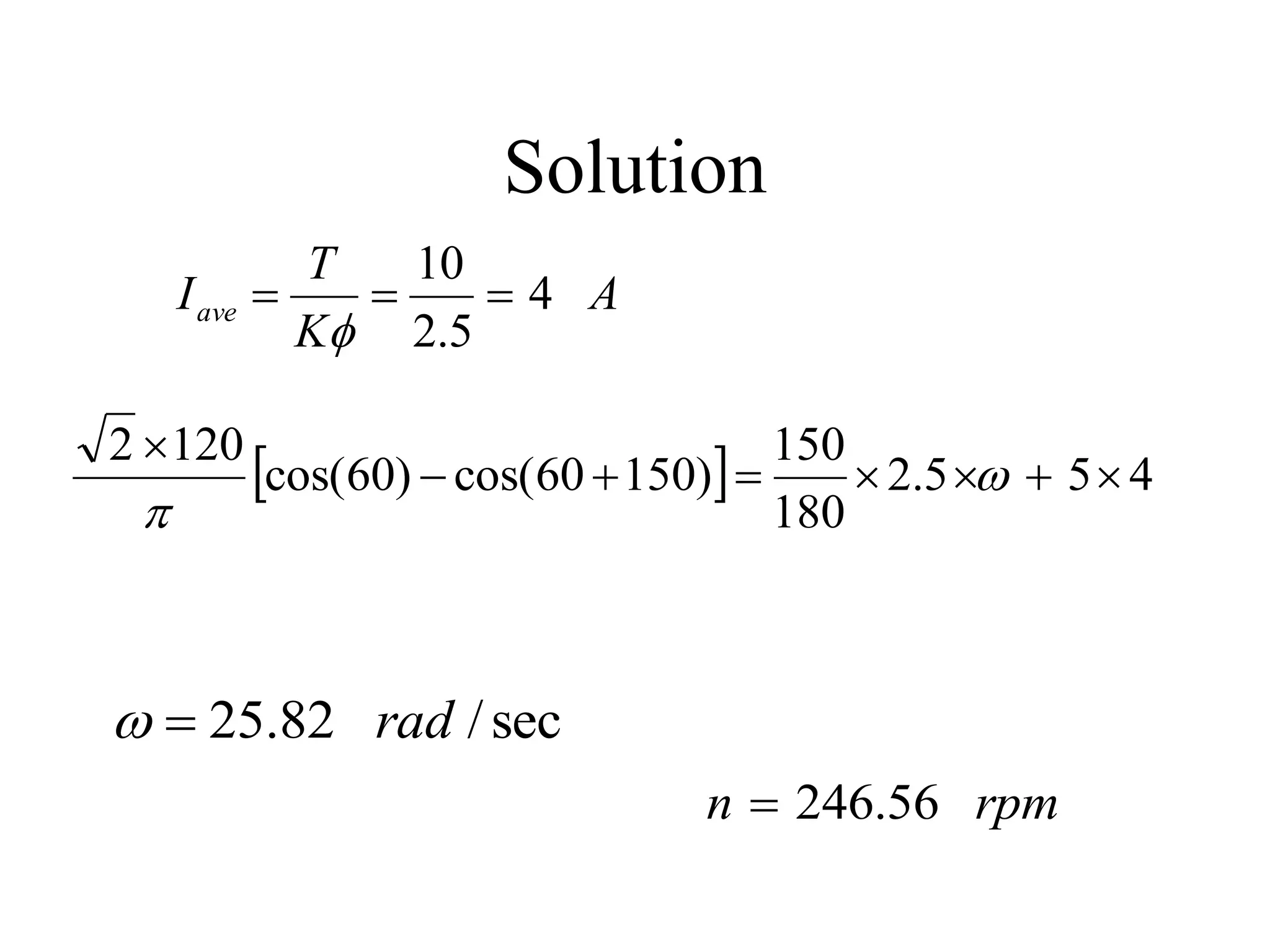
23. Solution
A
K
T
Iave 4
5
.
2
10




  4
5
5
.
2
360
150
)
150
60
cos(
)
60
cos(
2
120
2










sec
/
22
.
16 rad

 rpm
n 88
.
154

W
I
k
I
E
P ave
ave
a
d 162
4
22
.
16
5
.
2 




 

ave
a
max I
R
K
2
]
cos
[cos
2
V


 






24. Single-Phase, Full-Wave Drives
i1
i2
VS
S1 S4
S3 S2
Vt
Ra La
Ea

25. -200.00
-150.00
-100.00
-50.00
0.00
50.00
100.00
150.00
200.00
0 30 60 90 120 150 180 210 240 270 300 330 360
Angle
vt
v1
v2
Ea
i2
i1
vt
 

26. a
ave
a
t R
I
E
V ave



ave
a
a
a
s
ave
a
a
t
I
R
E
t
d
E
t
d
v
I
R
E
t
d
v


















 








1
2
2
0
  ave
a
a
max I
R
E
)
cos(
)
cos(
V









  ave
a
max I
R
K
)
cos(
)
cos(
V



 







27. Continuous Armature Current
i
Load3
Load2
Load1


180o
Angle
  ave
a
a
max I
R
E
)
180
cos(
)
cos(
V




 


ave
a
ave
a
a
max I
R
K
I
R
E
)
cos(
V
2





 



28. 3
1
2
4
Torque

Continuous Current
Discontinuous
Current
  ave
a
max I
R
K
)
cos(
)
cos(
V



 






ave
a
max I
R
K
)
cos(
V
2


 



29. Example 6.4
• For the motor in Example 6.3, assume
that the converter is a full-wave type.
The triggering angle of the converter is
60o, and the conduction period is 150o.
Calculate the motor speed and the
developed power.

30. Solution
A
K
T
Iave 4
5
.
2
10




  4
5
5
.
2
180
150
)
150
60
cos(
)
60
cos(
120
2










sec
/
82
.
25 rad


rpm
n 56
.
246


31. Example 6.5
• A dc separately excited motor has a
constant torque load of 60 NM. The
motor is driven by a full-wave converter
through a 120 V ac supply. The field
constant of the motor K = 2.5 and the
armature resistance is 2 W. Calculate
the triggering angle  for the motor to
operate at 200 rev/min. The motor
current is continuous.

32. Solution
 







































K
K
T
R
V
K
I
R
V
a
ave
a
max
1
max
1
2
cos
2
cos
ave
a
max
I
R
K
)
cos(
V
2

 



o
7
.
21
60
200
2
5
.
2
5
.
2
60
2
120
2
2
cos 1


















 




33. Waveform: Load Motor
(Continuous Current)
© M.A. El-Sharkawi, University of Washington 35
t
vt
vs
Ea
i
i1
i2
VS
S1 S2
D2 D1
Vt
Ra La
Ea
Freewheeling
 


34. a
ave
a
t R
I
E
V ave


ave
a
a
s
ave
a
a
t
I
R
E
t
d
v
I
R
E
t
d
v













1
diodes
ng
freewheeli
the
of
Because
2
2
0
  ave
a
a I
R
E
V


 )
cos(
)
cos(
max



  ave
a I
R
K
V


 




)
cos(
)
cos(
max
© M.A. El-Sharkawi, University of Washington 36

35.   ave
a I
R
K
V


 




)
cos(
)
cos(
max
© M.A. El-Sharkawi, University of Washington 37
  ave
a I
R
K
V


 




)
cos(
)
cos(
max
  ave
a I
R
K
V


 



1
)
cos(
max

36. Waveform: Unloaded
Motor
(Disontinuous Current)
© M.A. El-Sharkawi, University of Washington 38
i1
i2
VS
S1 S2
D2 D1
Vt
Ra La
Ea
0.25 0.255 0.26 0.265 0.27
Time (s)
0
-100
100
Vs Vt Ia
vt
vs
i
Freewheeling
Ea