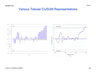
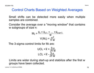
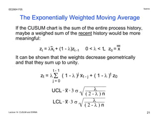
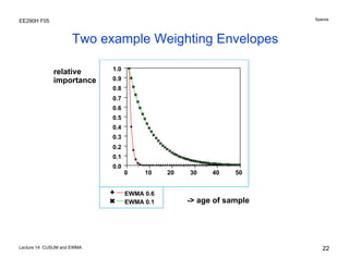
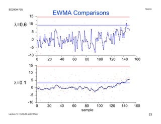
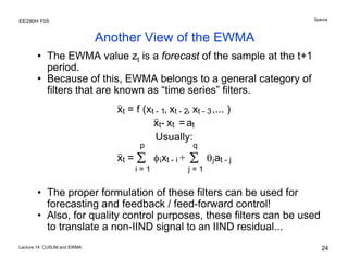
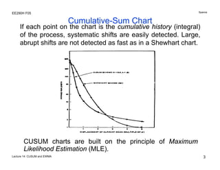
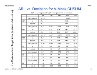
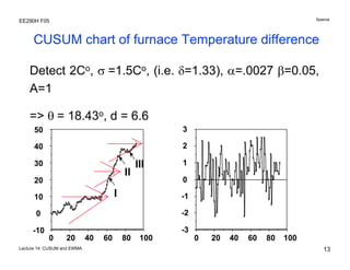
The document discusses various statistical process control charts for detecting small shifts in processes, including CUSUM (Cumulative Sum) charts and EWMA (Exponentially Weighted Moving Average) charts. CUSUM charts cumulatively sum process deviations and are more effective at detecting small shifts than Shewhart charts. EWMA charts create a weighted average of recent process data where older data is downweighted using an exponential factor. Both CUSUM and EWMA charts can be designed using maximum likelihood estimation and control limits to balance type I and type II error rates for detecting shifts of a given size.

1. Spanos
EE290H F05
CUSUM, MA and EWMA Control Charts
Increasing the sensitivity and getting ready for
automated control:
The Cumulative Sum chart, the Moving
Average and the Exponentially Weighted
Moving Average Charts.
Lecture 14: CUSUM and EWMA
1

2. Spanos
EE290H F05
Shewhart Charts cannot detect small shifts
The charts discussed so far are variations of the Shewhart
chart: each new point depends only on one subgroup.
Shewhart charts are sensitive to large process shifts.
The probability of detecting small shifts fast is rather small:
Fig 6-13 pp 195 Montgomery.
Lecture 14: CUSUM and EWMA
2

3. Spanos
EE290H F05
Cumulative-Sum Chart
If each point on the chart is the cumulative history (integral)
of the process, systematic shifts are easily detected. Large,
abrupt shifts are not detected as fast as in a Shewhart chart.
CUSUM charts are built on the principle of Maximum
Likelihood Estimation (MLE).
Lecture 14: CUSUM and EWMA
3

4. Spanos
EE290H F05
Maximum Likelihood Estimation
The "correct" choice of probability density function (pdf)
moments maximizes the collective likelihood of the
observations.
If x is distributed with a pdf(x,θ) with unknown θ, then θ can
be estimated by solving the problem:
m
max θ
Π pdf( xi,θ )
i=1
This concept is good for estimation as well as for comparison.
Lecture 14: CUSUM and EWMA
4

5. Spanos
EE290H F05
Maximum Likelihood Estimation Example
To estimate the mean value of a normal distribution, collect
the observations x1,x2, ... ,xm and solve the non-linear
programming problem:
⎧
⎫
⎧
2 ⎫
2
ˆ
ˆ
1 ⎛ x −μ ⎞
1 ⎛ x −μ ⎞ ⎞
⎛ 1
⎪m
⎪
m
− ⎜ i
− ⎜ i
⎟ ⎪
⎟
⎪
1
⎪
2⎝ σ ⎠
2 ⎝ σ ⎠ ⎟⎪
⎜
max μ ⎨Π
e
e
⎬ or min μ ⎨iΣ1 log⎜
ˆ
ˆ
⎟⎬
i =1 σ 2π
=
σ 2π
⎪
⎪
⎪
⎝
⎠⎪
⎪
⎪
⎩
⎭
⎩
⎭
Lecture 14: CUSUM and EWMA
5

6. Spanos
EE290H F05
MLE Control Schemes
If a process can have a "good" or a "bad" state (with the control
variable distributed with a pdf fG or fB respectively).
This statistic will be small when the process is "good" and large when
"bad":
m
f B(x i)
Σ log f G(xi)
i=1
m
m
log(Π pi ) = ∑ log( pi )
i =1
Lecture 14: CUSUM and EWMA
i =1
6

7. Spanos
EE290H F05
MLE Control Schemes (cont.)
Note that this counts from the beginning of the process. We
choose the best k points as "calibration" and we get:
m
k
f B(x i)
f B(x i)
S m = Σ log
- min k < m Σ log
>L
f G(x i)
f G(x i)
i=1
i=1
or
f B(x m)
S m = max (S m-1+log
, 0) > L
f G(x m)
This way, the statistic Sm keeps a cumulative score of all the
"bad" points. Notice that we need to know what the "bad"
process is!
Lecture 14: CUSUM and EWMA
7

8. Spanos
EE290H F05
The Cumulative Sum chart
If θ is a mean value of a normal distribution, is simplified to:
m
S m = Σ (x i - µ 0)
i=1
where μ0 is the target mean of the process. This can be
monitored with V-shaped or tabular “limits”.
Advantages
The CUSUM chart is very effective for small shifts and
when the subgroup size n=1.
Disadvantages
The CUSUM is relatively slow to respond to large shifts.
Also, special patterns are hard to see and analyze.
Lecture 14: CUSUM and EWMA
8

9. Spanos
EE290H F05
Shewhart small shift
Example
15
10
5
0
-5
-10
-15
UCL=13.4
µ0=-0.1
20
40
60
80
100
120
140
0
CUSUM small shift
0
LCL=-13.6
160
20
40
60
80
100
120
140
160
120
100
80
60
40
20
0
-20
-40
-60
Lecture 14: CUSUM and EWMA
9

10. Spanos
EE290H F05
The V-Mask CUSUM design
for standardized observations yi=(xi-μo)/σ
Need to set L(0) (i.e. the run length when the process is in
control), and L(δ) (i.e. the run-length for a specific deviation).
Figure 7-3 Montgomery pp 227
Lecture 14: CUSUM and EWMA
10

11. Spanos
EE290H F05
The V-Mask CUSUM design
for standardized observations yi=(xi-μo)/σ
δ is the amount of shift (normalized to σ) that we wish to detect with type I
error α and type II error β.
Α is a scaling factor: it is the horizontal distance between successive
points in terms of unit distance on the vertical axis.
2 ln 1- β
d=
2
α
δ
δ= Δ
θ = tan -1 δ
σx
2A
d
Lecture 14: CUSUM and EWMA
θ
11

12. Spanos
EE290H F05
ARL vs. Deviation for V-Mask CUSUM
Lecture 14: CUSUM and EWMA
12

13. Spanos
EE290H F05
CUSUM chart of furnace Temperature difference
Detect 2Co, σ =1.5Co, (i.e. δ=1.33), α=.0027 β=0.05,
A=1
=> θ = 18.43o, d = 6.6
50
3
40
2
30
II
20
III
0
I
10
1
-1
0
-2
-10
-3
0
20
Lecture 14: CUSUM and EWMA
40
60
80
100
0
20
40
60
80
100
13

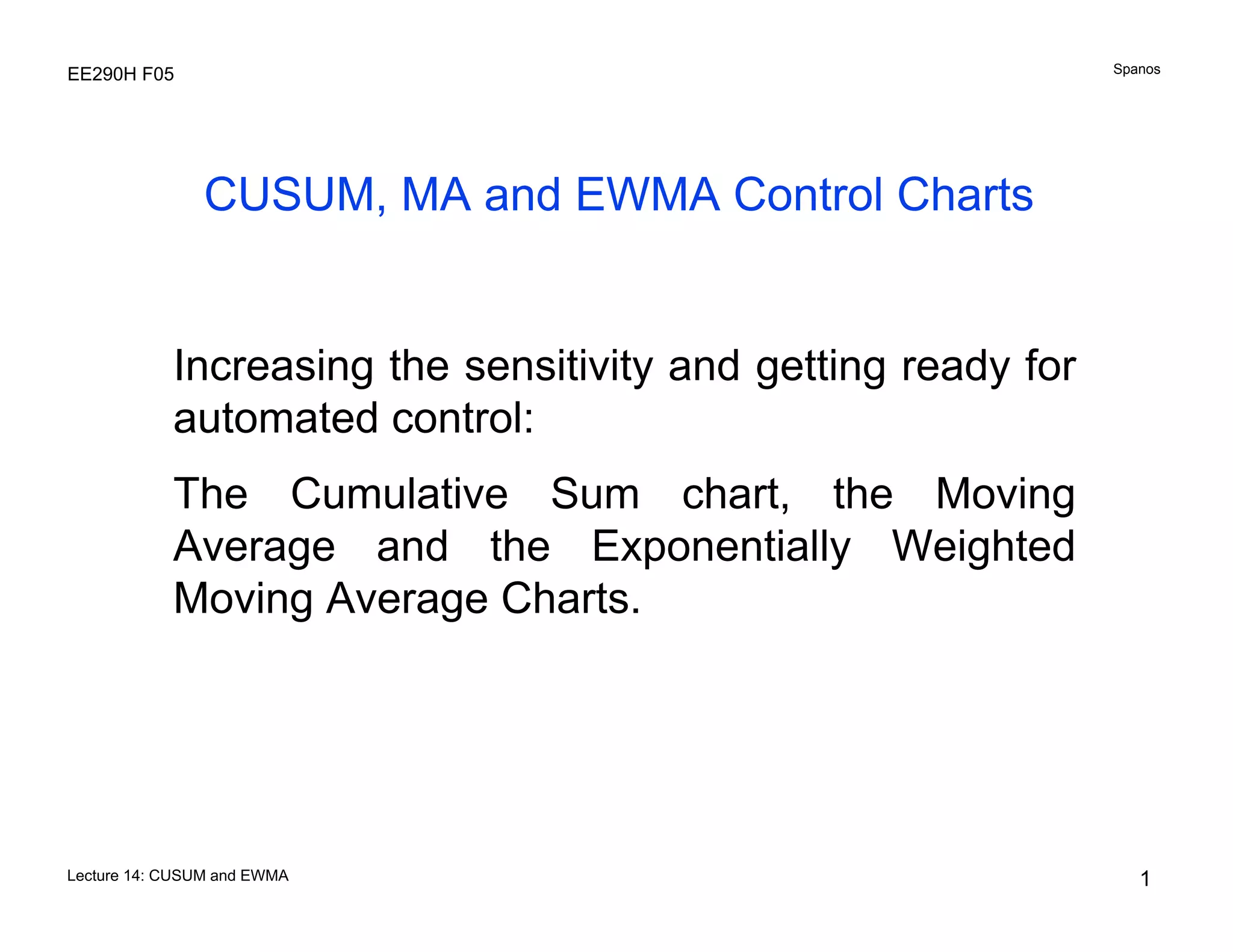
14. Spanos
EE290H F05
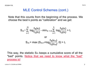
Tabular CUSUM
A tabular form is easier to implement in a CAM system
Ci+ = max [ 0, xi - ( μo + k ) + Ci-1+ ]
Ci-
= max [ 0, ( μo - k ) - xi +
h
Ci-1-
]
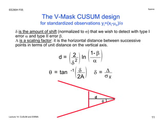
d
θ
C0+ = C0- = 0
k = (δ/2)/σ
h = dσxtan(θ)
Lecture 14: CUSUM and EWMA
14

15. Spanos
EE290H F05
Tabular CUSUM Example
Lecture 14: CUSUM and EWMA
15

16. Spanos
EE290H F05
Various Tabular CUSUM Representations
Lecture 14: CUSUM and EWMA
16

17. Spanos
EE290H F05
CUSUM Enhancements
To speed up CUSUM response one can use "modified" V
masks:
15
10
5
0
-5
0
20
40
60
80
100
Other solutions include the application of Fast Initial
Response (FIR) CUSUM, or the use of combined CUSUMShewhart charts.
Lecture 14: CUSUM and EWMA
17

18. Spanos
EE290H F05
General MLE Control Schemes
Since the MLE principle is so general, control
schemes can be built to detect:
• single or multivariate deviation in means
• deviation in variances
• deviation in covariances
An important point to remember is that MLE
schemes need, implicitly or explicitly, a definition of
the "bad" process.
The calculation of the ARL is complex but possible.
Lecture 14: CUSUM and EWMA
18

19. Spanos
EE290H F05
Control Charts Based on Weighted Averages
Small shifts can be detected more easily when multiple
samples are combined.
Consider the average over a "moving window" that contains
w subgroups of size n:
Mt =
x t + x t-1 + ... +x t-w+1
w
σ2
V(M t) = n w
The 3-sigma control limits for Mt are:
UCL = x + 3 σ
nw
LCL = x - 3 σ
nw
Limits are wider during start-up and stabilize after the first w
groups have been collected.
Lecture 14: CUSUM and EWMA
19

20. Spanos
EE290H F05
Example - Moving average chart
w = 10
15
10
5
0
-5
-10
0
20
40
60
80
100
120
140
160
sample
Lecture 14: CUSUM and EWMA
20

21. Spanos
EE290H F05
The Exponentially Weighted Moving Average
If the CUSUM chart is the sum of the entire process history,
maybe a weighed sum of the recent history would be more
meaningful:
zt = λxt + (1 - λ)zt -1
0 < λ < 1 z0 = x
It can be shown that the weights decrease geometrically
and that they sum up to unity.
t-1
z t = λ Σ ( 1 - λ )j x t - j + ( 1 - λ )t z 0
j=0
UCL = x + 3 σ
LCL = x - 3 σ
Lecture 14: CUSUM and EWMA
λ
(2-λ)n
λ
(2-λ)n
21

22. Spanos
EE290H F05
Two example Weighting Envelopes
relative
importance
1.0
0.9
0.8
0.7
0.6
0.5
0.4
0.3
0.2
0.1
0.0
0
10
EWMA 0.6
EWMA 0.1
Lecture 14: CUSUM and EWMA
20
30
40
50
-> age of sample
22

23. Spanos
EE290H F05
EWMA Comparisons
15
λ=0.6
10
5
0
-5
-10
0
20
40
60
0
20
40
60
80
100
120
140
160
80
100
sample
120
140
160
15
10
λ=0.1
5
0
-5
-10
Lecture 14: CUSUM and EWMA
23

24. Spanos
EE290H F05
Another View of the EWMA
• The EWMA value zt is a forecast of the sample at the t+1
period.
• Because of this, EWMA belongs to a general category of
filters that are known as “time series” filters.
xt = f (xt - 1, xt - 2, xt - 3 ,... )
xt- xt = at
Usually:
p
xt = Σ φixt - i +
i=1
q
Σ
θjat - j
j=1
• The proper formulation of these filters can be used for
forecasting and feedback / feed-forward control!
• Also, for quality control purposes, these filters can be used
to translate a non-IIND signal to an IIND residual...
Lecture 14: CUSUM and EWMA
24

25. Spanos
EE290H F05
Summary so far…
While simple control charts are great tools for visualizing
the process,it is possible to look at them from another
perspective:
Control charts are useful “summaries” of the process
statistics.
Charts can be designed to increase sensitivity without
sacrificing type I error.
It is this type of advanced charts that can form the
foundation of the automation control of the (near) future.
Next stop before we get there: multivariate and modelbased SPC!
Lecture 14: CUSUM and EWMA
25