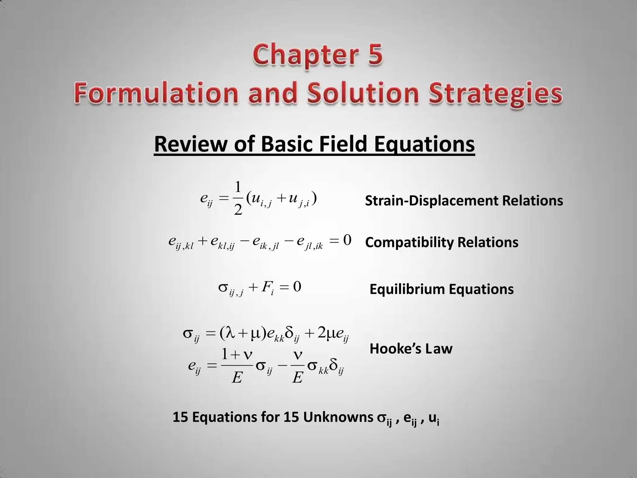
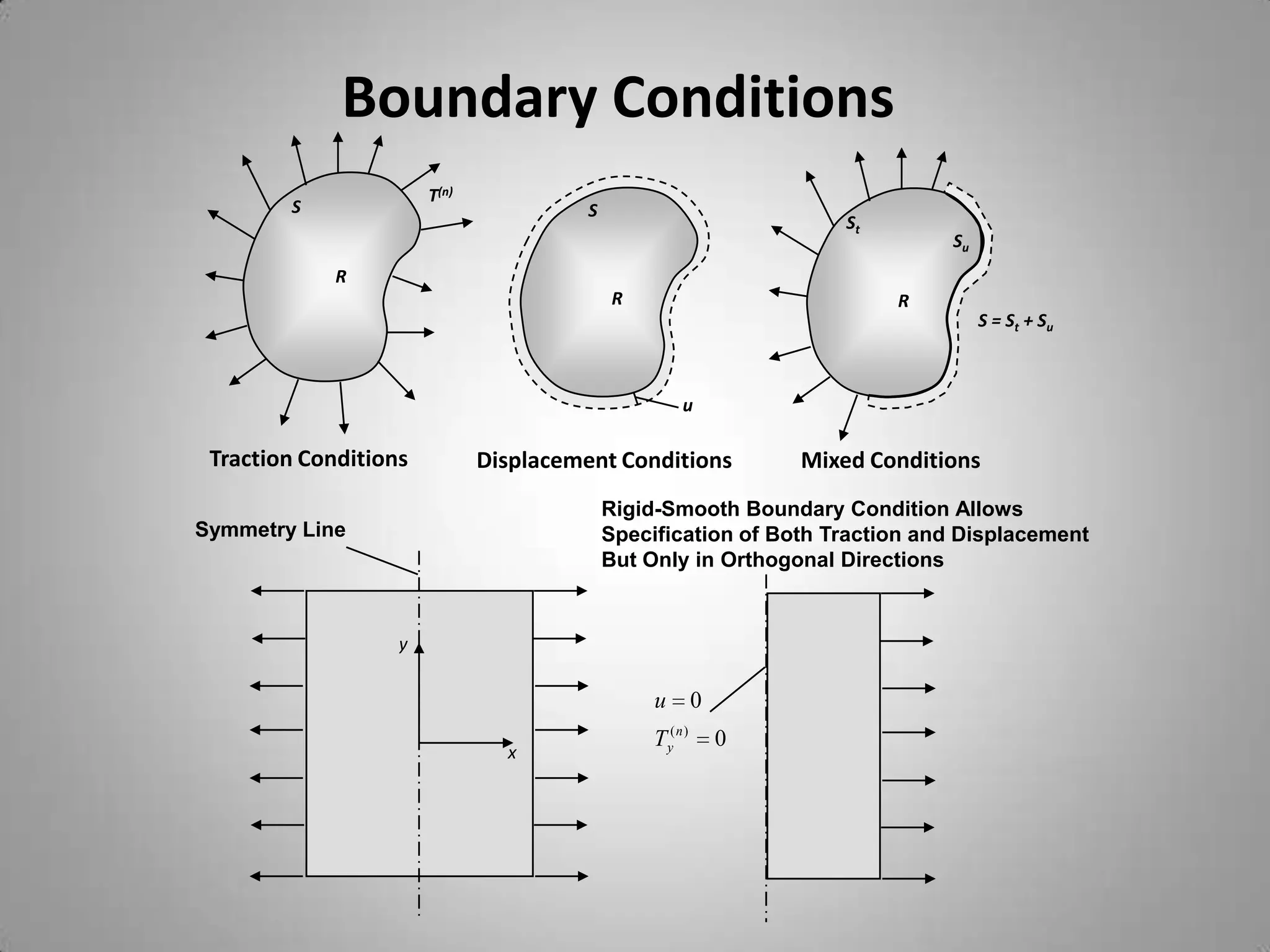
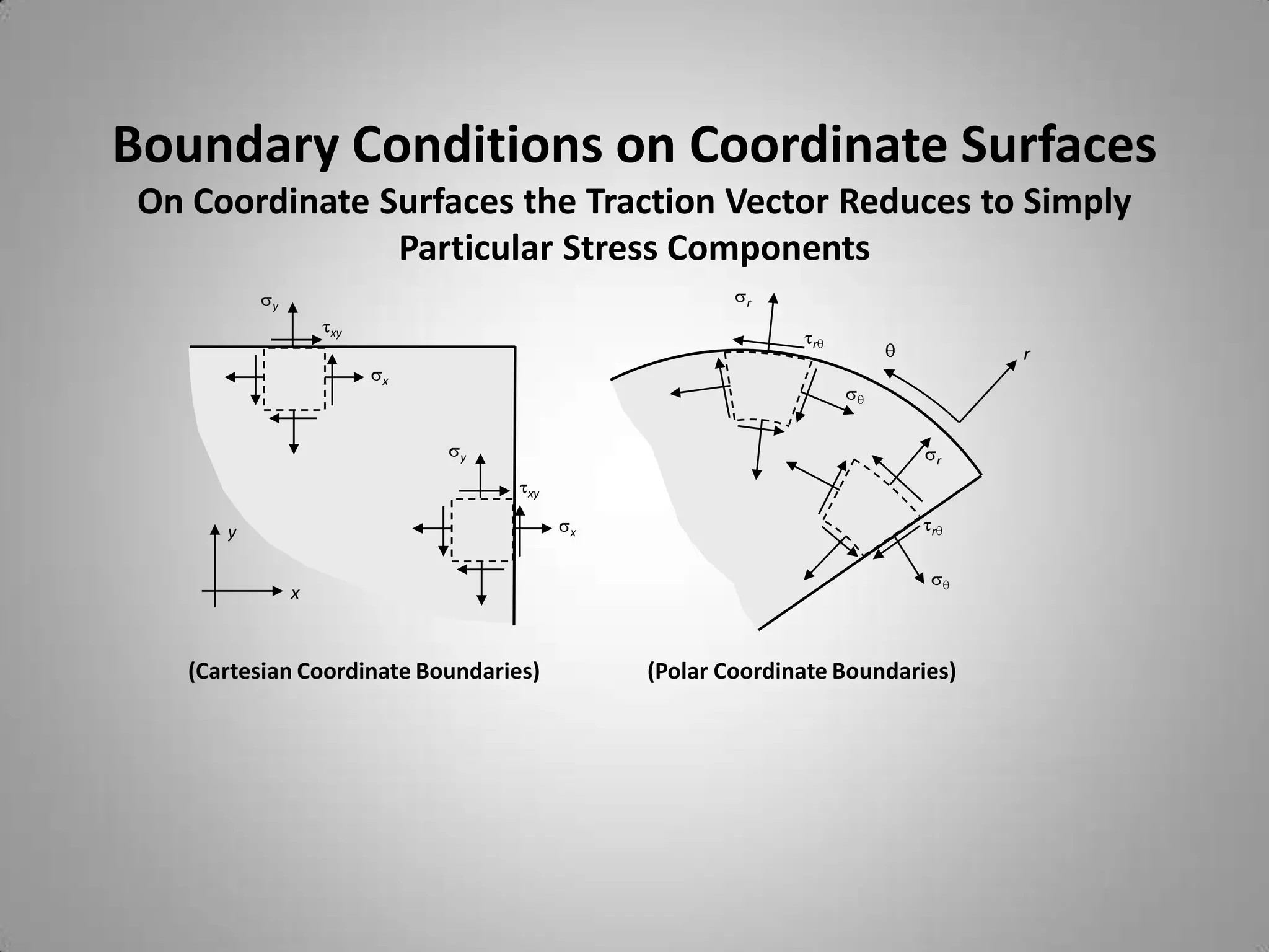
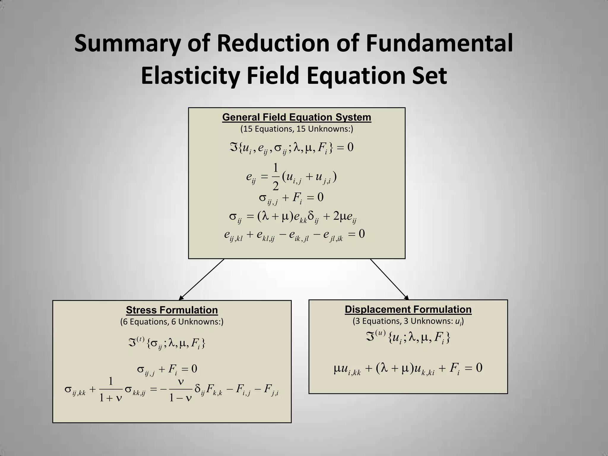
The document summarizes key equations in linear elasticity, including: 1. Strain-displacement relations, compatibility relations, and equilibrium equations form the general field equation system with 15 equations and 15 unknowns (displacements, strains, stresses). 2. Hooke's law relates stresses and strains. 3. Boundary conditions include traction, displacement, and mixed conditions and are specified on surfaces. 4. Fundamental problem classifications are the traction problem, displacement problem, and mixed problem. 5. The stress and displacement formulations eliminate unknowns to reduce the field equations to equations involving only stresses or only displacements.

1. Review of Basic Field Equations
1
eij (ui , j u j ,i ) Strain-Displacement Relations
2
eij , kl ekl,ij eik , jl e jl ,ik 0 Compatibility Relations
ij , j Fi 0 Equilibrium Equations
ij ( )ekk ij 2 eij
1 Hooke’s Law
eij ij kk ij
E E
15 Equations for 15 Unknowns ij , eij , ui

2. Boundary Conditions
T(n)
S S
St
Su
R
R R
S = St + Su
u
Traction Conditions Displacement Conditions Mixed Conditions
Rigid-Smooth Boundary Condition Allows
Symmetry Line Specification of Both Traction and Displacement
But Only in Orthogonal Directions
y
u 0
Ty(n ) 0
x

3. Boundary Conditions on Coordinate Surfaces
On Coordinate Surfaces the Traction Vector Reduces to Simply
Particular Stress Components
y r
xy
r
r
x
y r
xy
y x r
x
(Cartesian Coordinate Boundaries) (Polar Coordinate Boundaries)

4. Boundary Conditions on General Surfaces
On General Non-Coordinate Surfaces Traction Vector Will Not
Reduce to Individual Stress Components and General Form of
Traction Vector Must Then Be Used
n
y
Tx( n ) x nx xy ny S cos
Ty( n ) xy nx y ny S sin
S
x
Two-Dimensional Example

5. Example Boundary Conditions
Traction Free Condition
Fixed Condition
y u=v=0
Traction Condition
Tx( n ) x S, Ty( n ) xy 0 Traction Condition
Tx( n) xy 0, Ty( n) y S
S
x l
b S
Tx(n ) 0
a Ty(n ) 0 y
x
Fixed Condition
Traction Free Condition
u=v=0 Traction Free Condition
Tx( n) xy 0, Ty( n) y 0
Coordinate Surface Boundaries Non-Coordinate Surface
Boundary

6. Interface Boundary Conditions
(1)
Material (1): ij , u i(1)
n Interface Conditions:
Perfectly Bonded,
s Slip Interface, Etc.
( 2)
Material (2): ij , ui( 2)
Embedded Fiber or Rod Layered Composite Plate Composite Cylinder or Disk

7. Fundamental Problem Classifications
Problem 1 (Traction Problem) Determine the distribution of T(n)
S
displacements, strains and stresses in the interior of an elastic
body in equilibrium when body forces are given and the
R
distribution of the tractions are prescribed over the surface of the
body,
Ti ( n ) ( xi( s ) ) f i ( xi( s ) )
Problem 2 (Displacement Problem) Determine the distribution of
displacements, strains and stresses in the interior of an elastic body S
in equilibrium when body forces are given and the distribution of
the displacements are prescribed over the surface of the body. R
ui ( xi( s ) ) g i ( xi( s ) )
u
Problem 3 (Mixed Problem) Determine the distribution of
displacements, strains and stresses in the interior of an elastic body St
in equilibrium when body forces are given and the distribution of Su
the tractions are prescribed as per (5.2.1) over the surface St and R
the distribution of the displacements are prescribed as per (5.2.2)
over the surface Su of the body (see Figure 5.1).

8. Stress Formulation
Eliminate Displacements and Strains from
Fundamental Field Equation Set
(Zero Body Force Case)
Compatibility in Terms of Stress:
Equilibrium Equations Beltrami-Michell Compatibility Equations
2
x yx zx
0 (1 ) 2
x ( x y z ) 0
x y z x2
2
2
xy y zy (1 ) ( ) 0
0 y
y 2 x y z
x y z 2
2
(1 ) z ( x y z ) 0
xz yz z
0 z2
2
x y z 2
(1 ) xy ( x y z ) 0
x y
2
2
(1 ) yz ( x y z ) 0
y z
2
2
(1 ) zx ( x y z ) 0
z x
6 Equations for 6 Unknown Stresses

9. Displacement Formulation
Eliminate Stresses and Strains from
Fundamental Field Equation Set
(Zero Body Force Case)
Equilibrium Equations in Terms of Displacements:
Navier’s/Lame’s Equations
2 u v w
u ( ) 0
x x y z
2 u v w
v ( ) 0
y x y z
2 u v w
w ( ) 0
z x y z
3 Equations for 3 Unknown Displacements

10. Summary of Reduction of Fundamental
Elasticity Field Equation Set
General Field Equation System
(15 Equations, 15 Unknowns:)
{ui , eij , ij ; , , Fi } 0
1
eij (ui , j u j ,i )
2
ij , j Fi 0
ij ( )ekk ij 2 eij
eij ,kl ekl,ij eik , jl e jl ,ik 0
Stress Formulation Displacement Formulation
(6 Equations, 6 Unknowns:) (3 Equations, 3 Unknowns: ui)
(u )
(t )
{ {ui ; , , Fi }
ij ; , , Fi }
ij , j Fi 0 ui ,kk ( )u k ,ki Fi 0
1
ij ,kk kk ,ij ij Fk ,k Fi , j F j ,i
1 1

11. Principle of Superposition
(1)
For a given problem domain, if the state { ij , eij1) , ui(1) } is a solution to the fundamental
(
elasticity equations with prescribed body forces Fi (1) and surface tractions Ti (1) , and the
( 2)
state { ij , eij2) , ui( 2) } is a solution to the fundamental equations with prescribed body
(
(1) ( 2)
forces Fi ( 2 ) and surface tractions Ti ( 2 ) , then the state { ij ij , eij1)
(
eij2) , ui(1)
(
ui( 2) }
will be a solution to the problem with body forces Fi (1) Fi ( 2 ) and surface tractions
Ti (1) Ti ( 2 ) .
(1)+(2) = (1) + (2)
(1)
{ ij , eij1) , ui(1) }
(
( 2)
{ (1)
ij
( 2)
ij , eij1)
(
eij2) , ui(1)
(
ui( 2) } { ij , eij2) , ui( 2) }
(

12. Saint-Venant’s Principle
The stress, strain and displacement fields due to two different
statically equivalent force distributions on parts of the body far
away from the loading points are approximately the same
FR T(n)
P P P P P P
2 2 3 3 3
S*
(1) (2) (3)
Boundary loading T(n) would produce detailed
and characteristic effects only in the vicinity of
S*. Away from S* the stresses would generally
depend more on the resultant FR of the tractions
Stresses approximately the same rather than on the exact distribution

13. General Solution Strategies Used to
Solve Elasticity Field Equations
Direct Method - Solution of field equations by direct integration. Boundary
conditions are satisfied exactly. Method normally encounters significant
mathematical difficulties thus limiting its application to problems with simple
geometry.
Inverse Method - Displacements or stresses are selected that satisfy field equations.
A search is then conducted to identify a specific problem that would be solved by
this solution field. This amounts to determine appropriate problem geometry,
boundary conditions and body forces that would enable the solution to satisfy all
conditions on the problem. It is sometimes difficult to construct solutions to a
specific problem of practical interest.
Semi-Inverse Method - Part of displacement and/or stress field is specified, while
the other remaining portion is determined by the fundamental field equations
(normally using direct integration) and the boundary conditions. It is often the case
that constructing appropriate displacement and/or stress solution fields can be
guided by approximate strength of materials theory. The usefulness of this approach
is greatly enhanced by employing Saint-Venant’s principle, whereby a complicated
boundary condition can be replaced by a simpler statically equivalent distribution.

14. Mathematical Techniques Used to
Solve Elasticity Field Equations
Analytical Solution Procedures
- Power Series Method
- Fourier Method
- Integral Transform Method
- Complex Variable Method
Approximate Solution Procedures
- Ritz Method
Numerical Solution Procedures
- Finite Difference Method (FDM)
- Finite Element Method (FEM)
- Boundary Element Method (BEM)