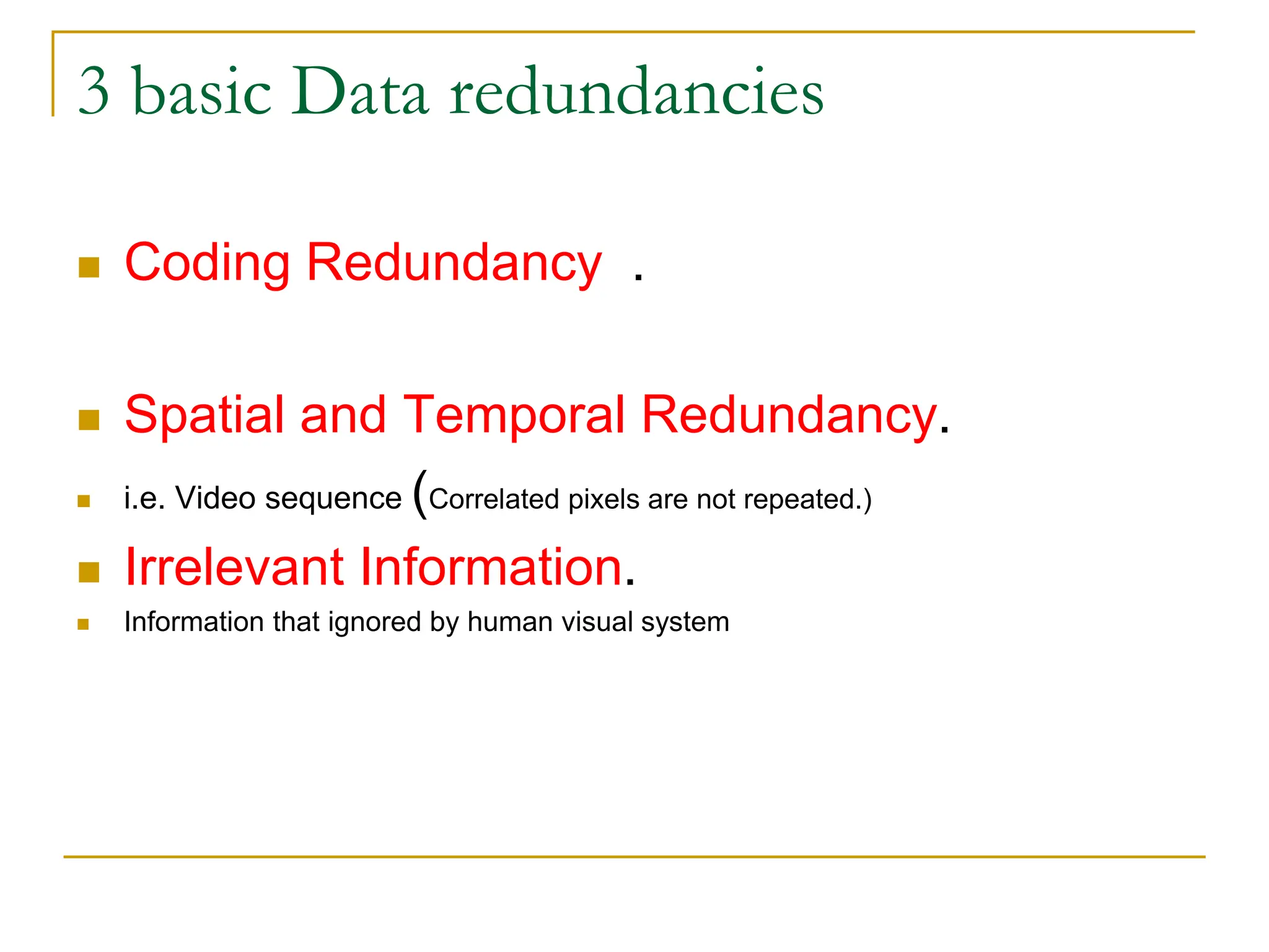
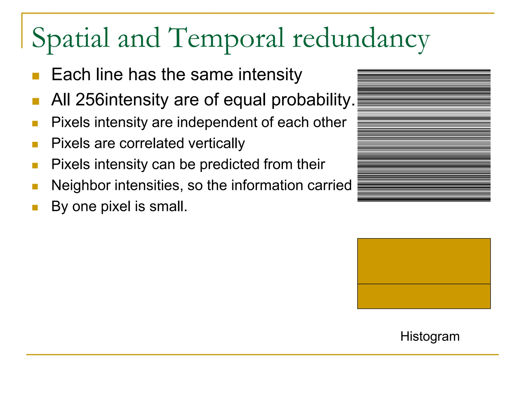
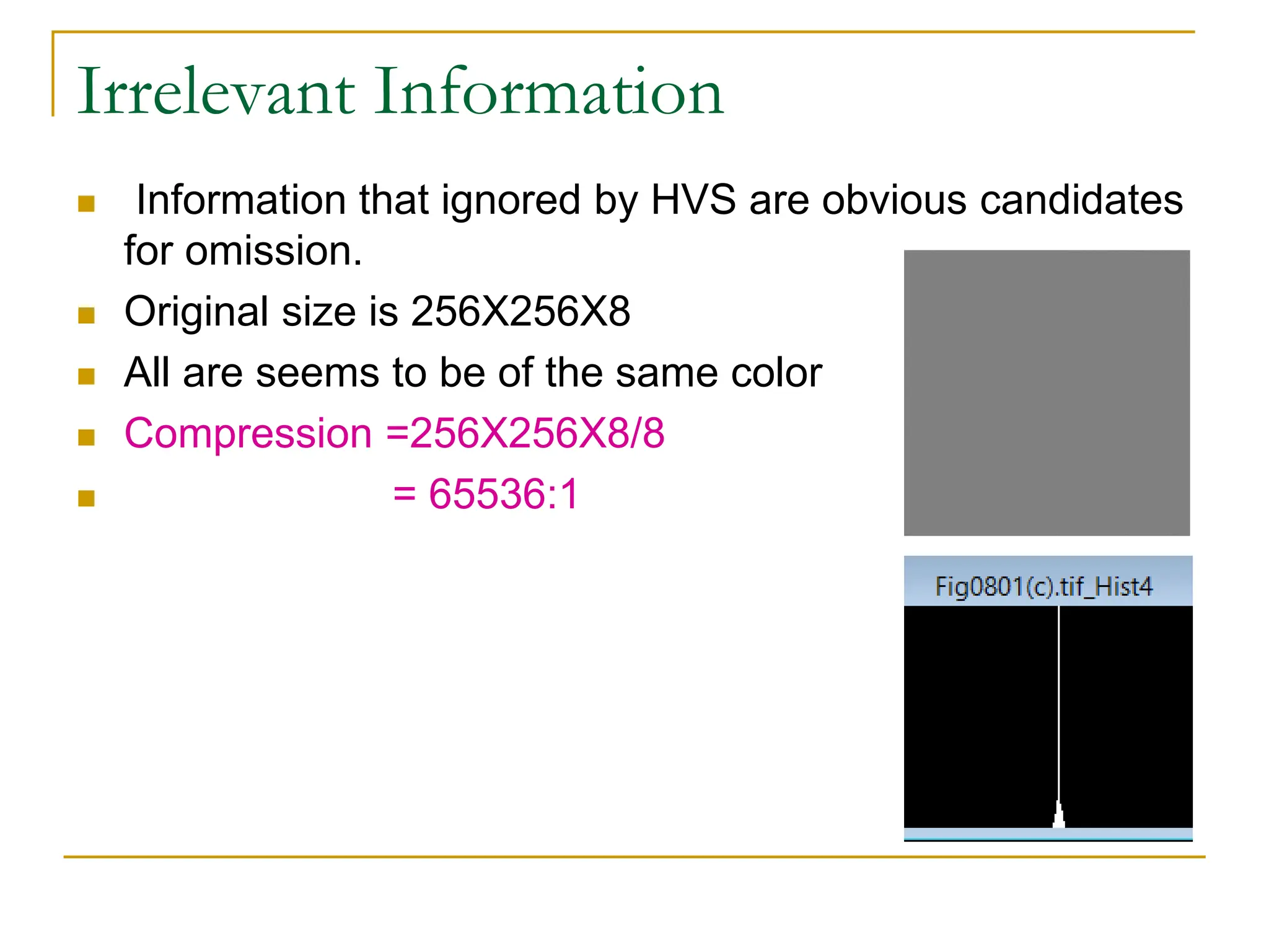
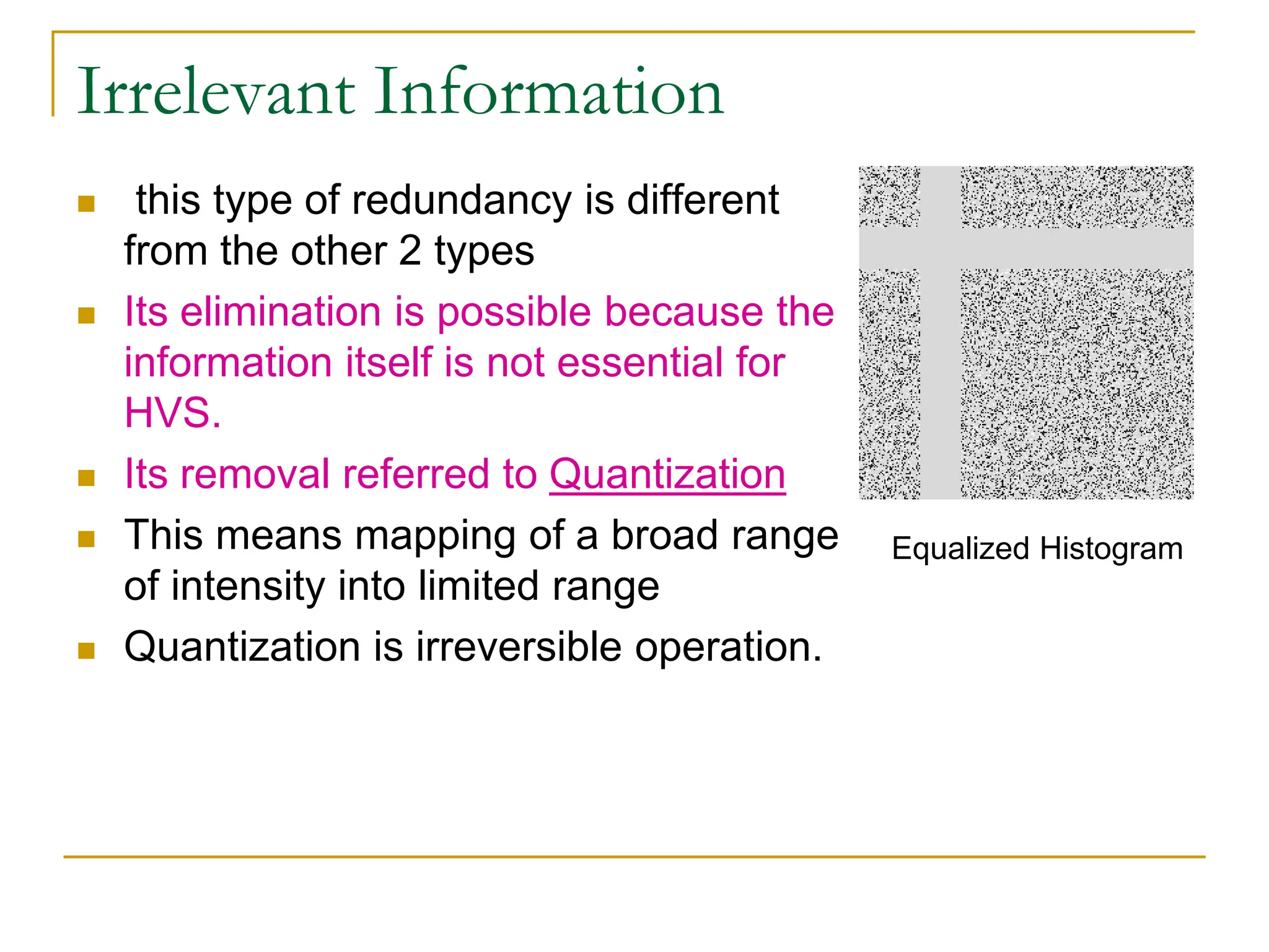
This document discusses various methods of image compression. It begins by defining image compression as reducing the amount of data required to represent a digital image. The main methods of compression are by removing redundant data from the image. The document then discusses three main types of data redundancy that can be reduced: coding redundancy, spatial/temporal redundancy, and irrelevant information redundancy. Coding redundancy refers to inefficient coding of pixel values and can be reduced using techniques like Huffman coding or arithmetic coding. Spatial/temporal redundancy occurs from correlations between neighboring pixel values, while irrelevant information redundancy refers to data that is ignored by the human visual system. 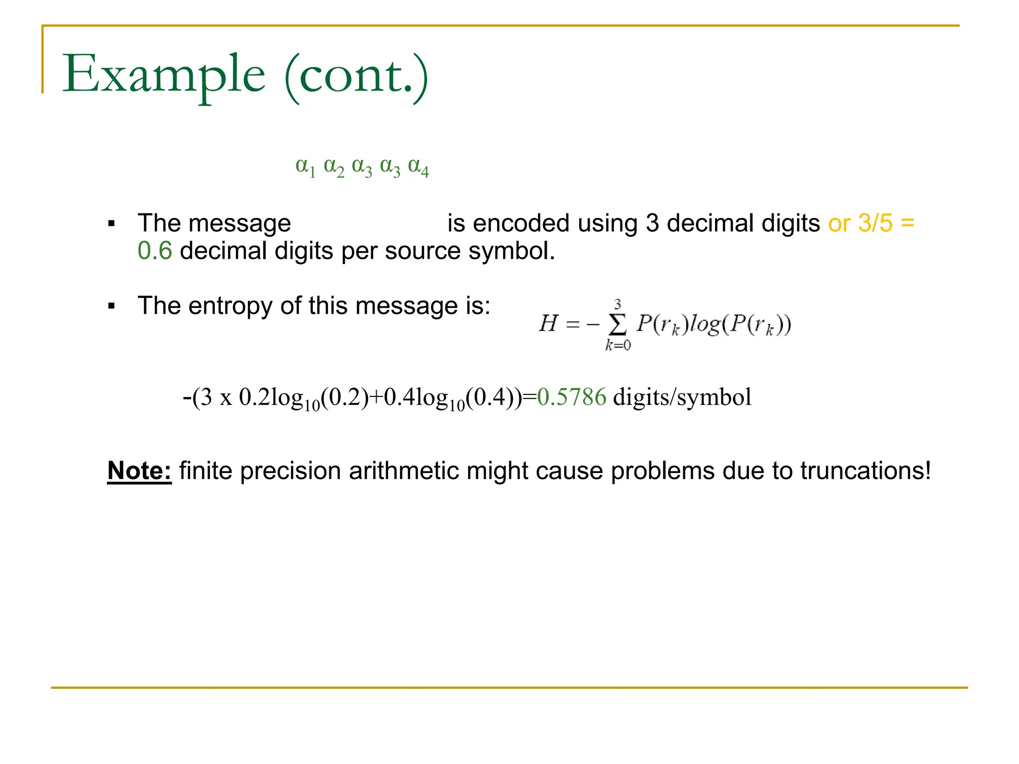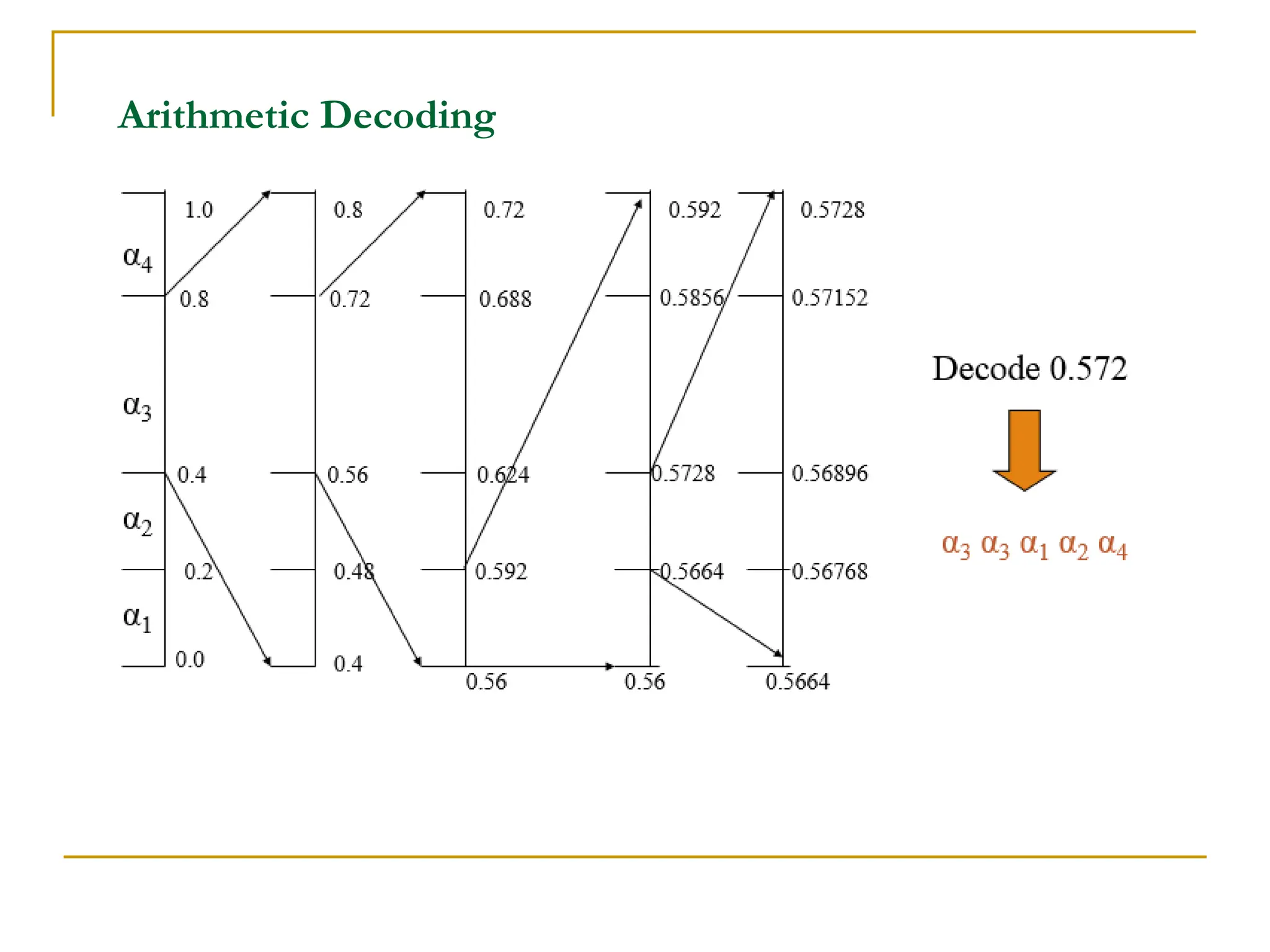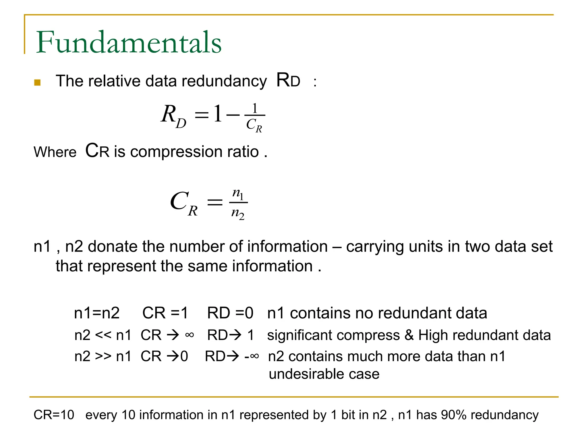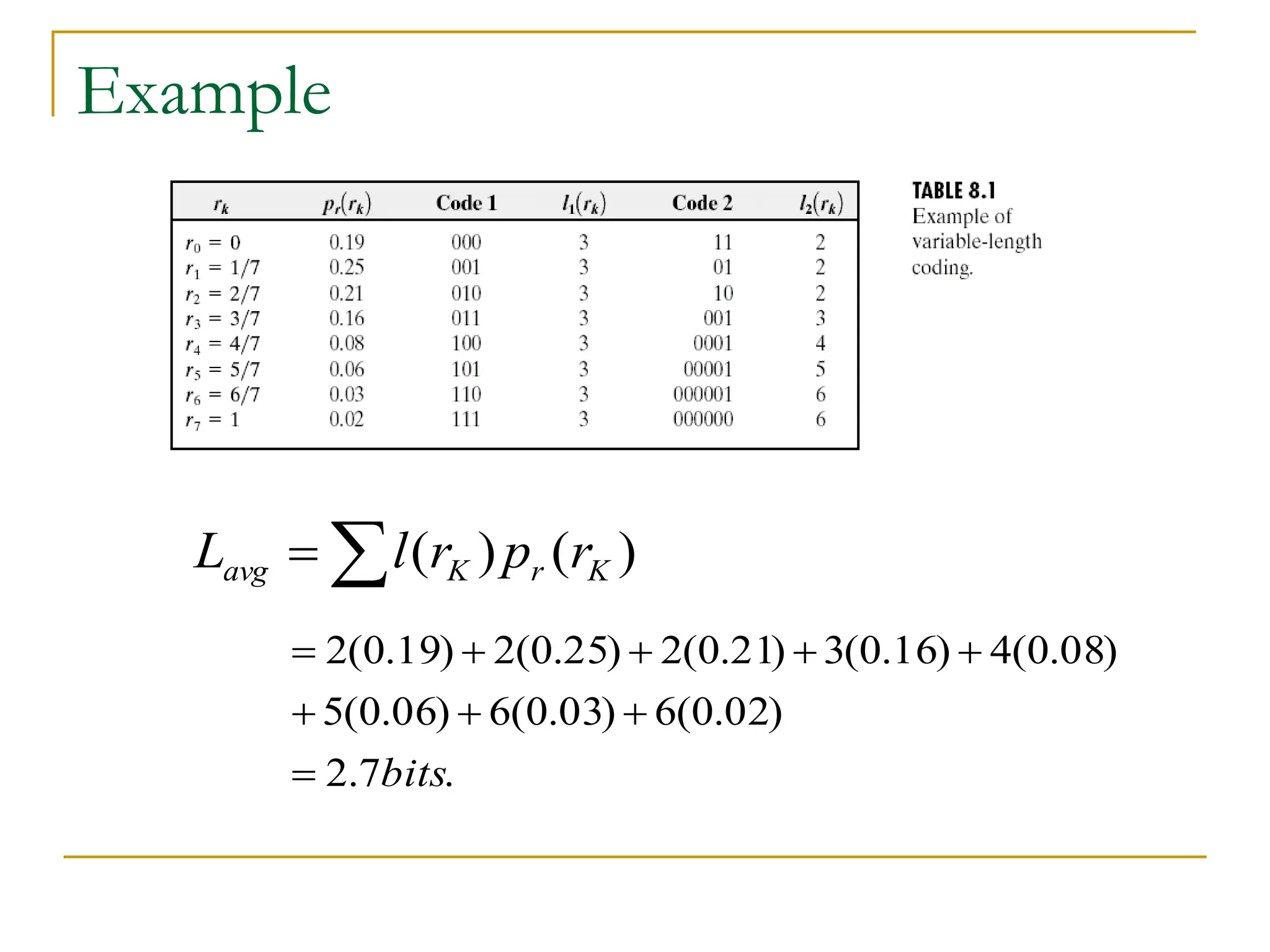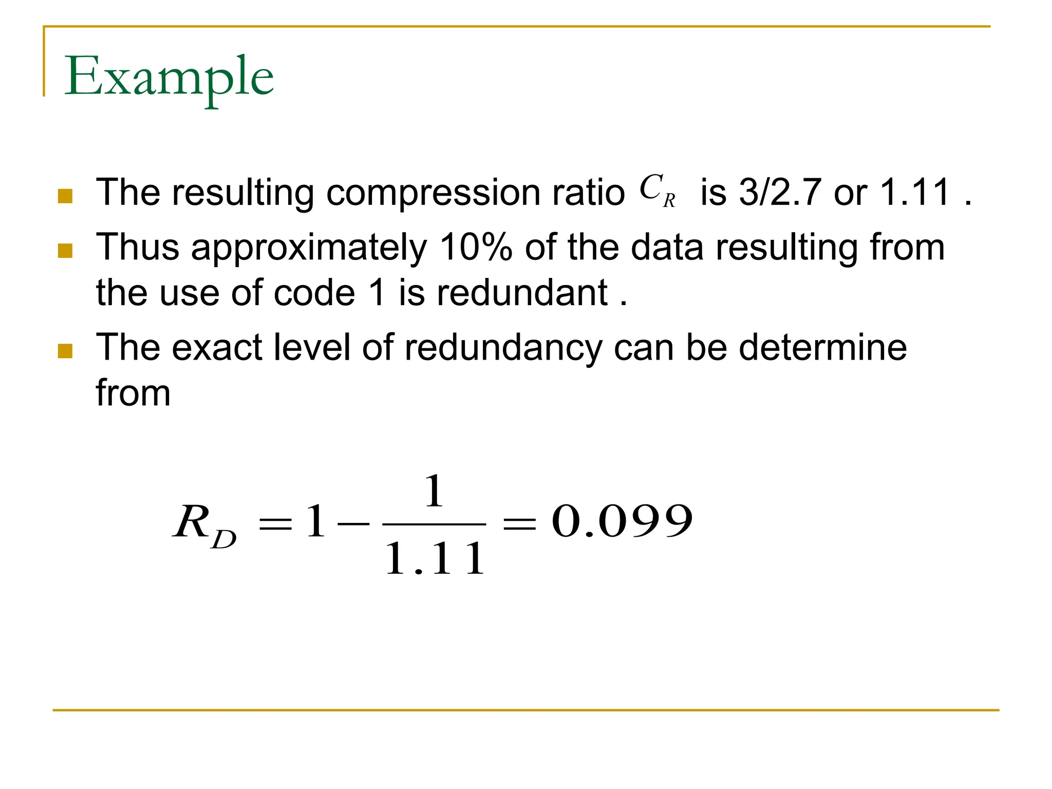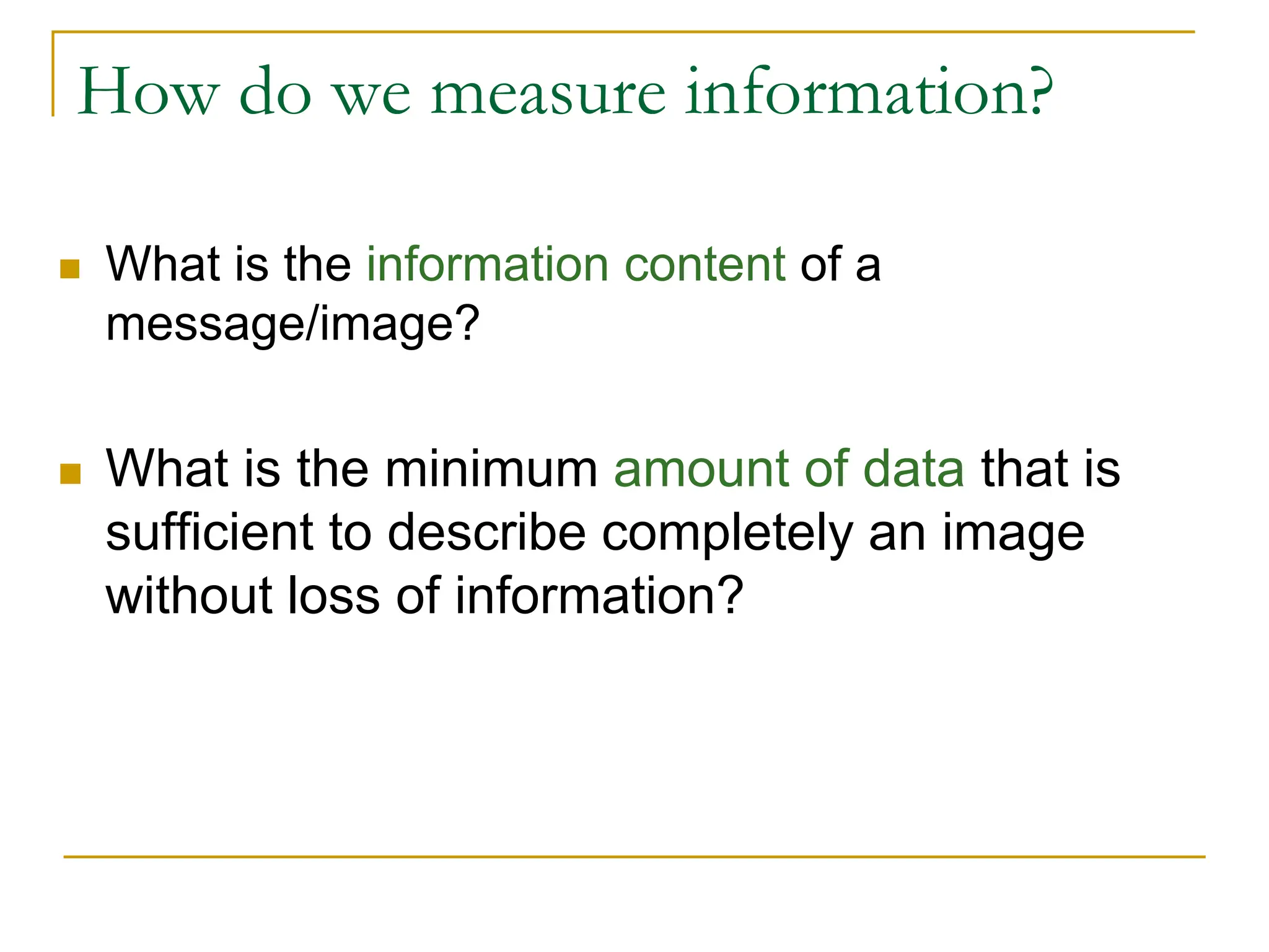The document provides examples and formulas for measuring compression ratio, data redundancy, and estimating the information content of

1. Image Compression

2. Preview
 Methods of compressing data prior to storage and / or
transmission are of significant practical and commercial
 Image compression addresses the problem of reducing
the amount of data required to a digital image .
 The underlying basis of the reduction process is the
removal of redundant data .

3. Fundamentals
 The data compression refers to the process of reducing
the amount of data required to represent a given quantity
of information .
 The difference of data and information .
 Data are the means by which information is conveyed .
 Data redundancy is a central issue in digital image
compression

4. Fundamentals
 The relative data redundancy RD :
Where CR is compression ratio .
n1 , n2 donate the number of information – carrying units in two data set
that represent the same information .
n1=n2 CR =1 RD =0 n1 contains no redundant data
n2 << n1 CR  ∞ RD 1 significant compress & High redundant data
n2 >> n1 CR 0 RD -∞ n2 contains much more data than n1
undesirable case
CR=10 every 10 information in n1 represented by 1 bit in n2 , n1 has 90% redundancy
1
1 R
D C
R  
1
2
n
R n
C 

5. 3 basic Data redundancies
 Coding Redundancy .
 Spatial and Temporal Redundancy.
 i.e. Video sequence (Correlated pixels are not repeated.)
 Irrelevant Information.
 Information that ignored by human visual system

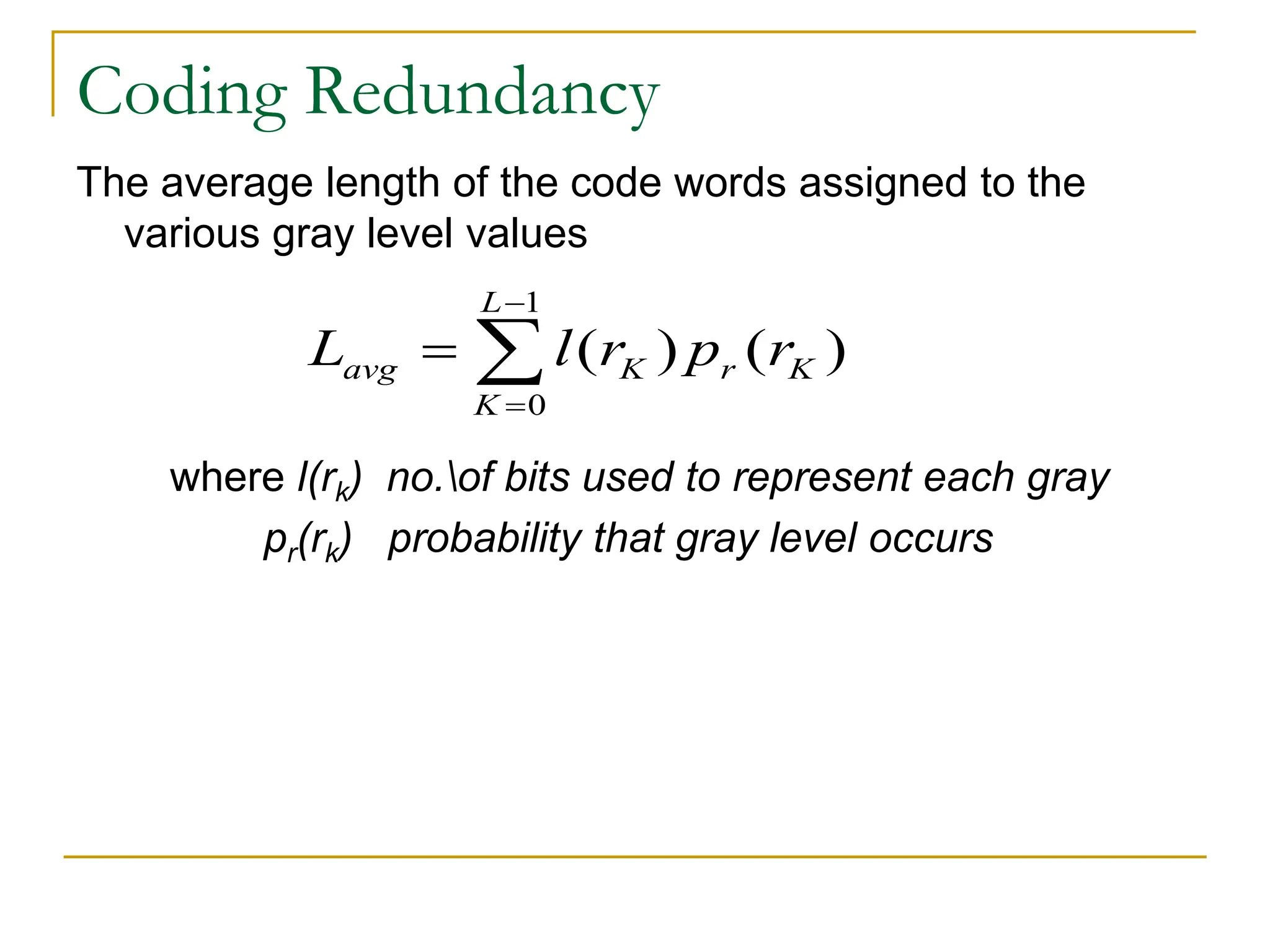
6. Coding Redundancy
 Lets assume , that a discrete random variable rK in the
interval [0 , 1] represents the gray levels of an image and
each rK occurs with probability
k=0,1,2,……L-1
Where L is the number gray levels ,
nK is the number of times that the Kth gray level appears in
image .
n is the total number of pixel in the image .
( ) K
n
r K n
P r 
( )
r K
P r

7. Coding Redundancy
The average length of the code words assigned to the
various gray level values
where l(rk) no.of bits used to represent each gray
pr(rk) probability that gray level occurs
1
0
( ) ( )
L
avg K r K
K
L l r p r


 

8. )
(
)
( K
r
K
avg r
p
r
l
L 

.
7
.
2
)
02
.
0
(
6
)
03
.
0
(
6
)
06
.
0
(
5
)
08
.
0
(
4
)
16
.
0
(
3
)
21
.
0
(
2
)
25
.
0
(
2
)
19
.
0
(
2
bits









Example

9. Example
 The resulting compression ratio is 3/2.7 or 1.11 .
 Thus approximately 10% of the data resulting from
the use of code 1 is redundant .
 The exact level of redundancy can be determine
from
R
C
099
.
0
11
.
1
1
1 


D
R

10. Spatial and Temporal redundancy
 Each line has the same intensity
 All 256intensity are of equal probability.
 Pixels intensity are independent of each other
 Pixels are correlated vertically
 Pixels intensity can be predicted from their
 Neighbor intensities, so the information carried
 By one pixel is small.
Histogram

11. Irrelevant Information
 Information that ignored by HVS are obvious candidates
for omission.
 Original size is 256X256X8
 All are seems to be of the same color
 Compression =256X256X8/8
 = 65536:1

12. Irrelevant Information
 this type of redundancy is different
from the other 2 types
 Its elimination is possible because the
information itself is not essential for
HVS.
 Its removal referred to Quantization
 This means mapping of a broad range
of intensity into limited range
 Quantization is irreversible operation.
Equalized Histogram

13. How do we measure information?
 What is the information content of a
message/image?
 What is the minimum amount of data that is
sufficient to describe completely an image
without loss of information?

14. Modeling Information
Information generation is assumed to be a
probabilistic process.
Idea: associate information with probability!
Note: I(E)=0 when P(E)=1 The event always occurs
A random event E with probability P(E) contains:

15. How much information does a pixel contain?
Suppose that gray level values are
generated by a random variable, then rk
contains:
units of information!

16. 
Average information content of an image:
units/pixel
1
0
( )Pr( )
L
k k
k
E I r r


 
using
How much information does an image contain?
(assumes statistically independent random events)
Entropy
It is not possible to code an image with fewer than H bits/pixel

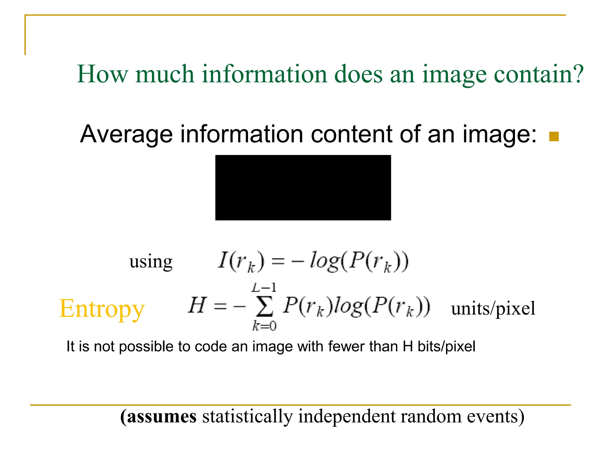
17. Example:
 H = -[.25 log2 0.25 +.47 log2 0.47 +
 .25 log2 0.25 + .03 log2 0.03]
 = [-0.25(-2) +.47(-1.09) + .25(-2) +.03(-5.06)]
 = 1.6614 bits/pixel
 What about H for the second type of redundancy?

18. Fidelity Criteria
 Objective fidelity criterion
Loss of information – compress – decompress .
 Subjective fidelity criteria
Quality of image .

19. Fidelity criteria
 Irrelevant information represents a loss, so we need a mean of
quantifying the nature of loss
 When the level of information loss can be expressed as a function of
the original or input image and the compressed and decompressed
output image , it is based on an objective fidelity criterion .
 Example : the error at any x,y
 The total error
 






1
0
1
0
)
,
(
)
,
(
ˆ
M
x
N
y
y
x
f
y
x
f
)
,
(
)
,
(
ˆ
)
,
( y
x
f
y
x
f
y
x
e 

Approximate Original

20.  The square root
 The mean square signal – to – noise
 
2
1
0
1
0
1
0
1
0
2
)
,
(
)
,
(
ˆ
)
,
(
ˆ
  










M
x
N
y
M
x
N
y
rms
y
x
f
y
x
f
y
x
f
SNR
 
2
1
2
1
0
1
0
)
,
(
)
,
(
ˆ
1








  





M
x
N
y
y
x
f
y
x
f
MN
rms
e

21. Fidelity Criteria(Subjective)

22. Huffman Coding (coding redundancy)
 A variable-length coding technique.
 Optimal code (i.e., minimizes the number of
code symbols per source symbol).
 Assumption: symbols are encoded one at a
time!

23. Huffman Coding (cont’d)
• Forward Pass
1. Sort probabilities per symbol
2. Combine the lowest two probabilities
3. Repeat Step2 until only two probabilities remain.

24. Huffman Coding (cont’d)
 Backward Pass
Assign code symbols going backwards

25. Huffman Coding (cont’d)
 Lavg using Huffman coding:
 Lavg assuming binary codes:

26. Huffman Coding/Decoding

After the code has been created,
coding/decoding can be implemented using a
look-up table.

Note that decoding is done unambiguously.

27. Arithmetic (or Range) Coding
(coding redundancy)
 Instead of encoding source symbols one
at a time, sequences of source symbols
are encoded together.
 There is no one-to-one correspondence
between source symbols and code words.
 Slower than Huffman coding but
typically achieves better compression.

28. Arithmetic Coding (cont.)
 A sequence of source symbols is
assigned to a sub-interval in [0,1) which
corresponds to an arithmetic code, e.g.,
 We start with the interval [0, 1) ; as the
number of symbols in the message
increases, the interval used to represent
the message becomes smaller.
arithmetic code

29. Arithmetic Coding (cont.)
Encode message: α1 α2 α3 α3 α4
0 1
1) Start with interval [0, 1)
2) Subdivide [0, 1) based on the probabilities of αi
3) Update interval by processing source symbols

30. Example

31. Example (cont.)
▪ The message is encoded using 3 decimal digits or 3/5 =
0.6 decimal digits per source symbol.
▪ The entropy of this message is:
Note: finite precision arithmetic might cause problems due to truncations!
α1 α2 α3 α3 α4
-(3 x 0.2log10(0.2)+0.4log10(0.4))=0.5786 digits/symbol

32. Arithmetic Decoding