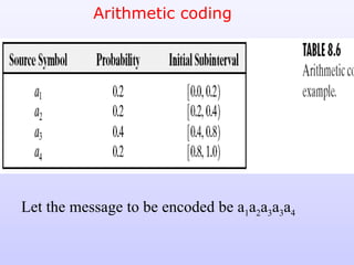
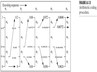
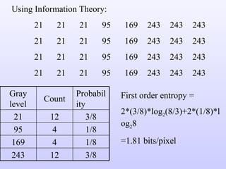
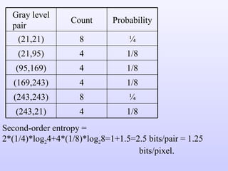
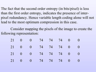
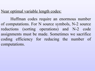
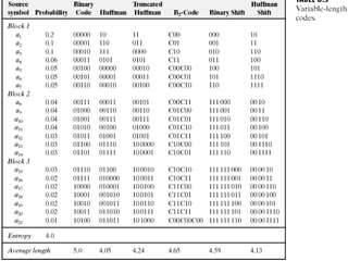
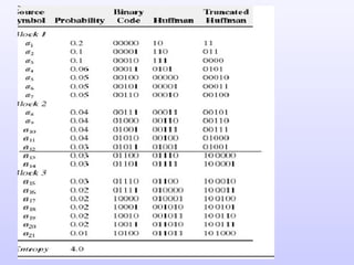
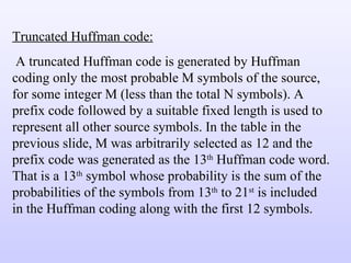
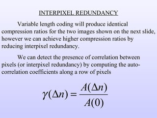
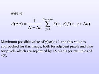
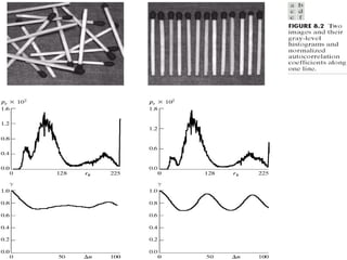
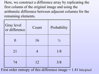
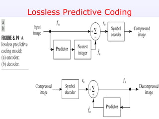
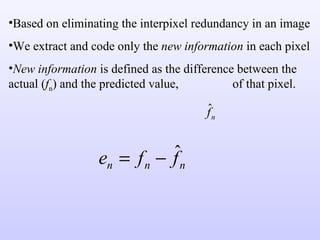
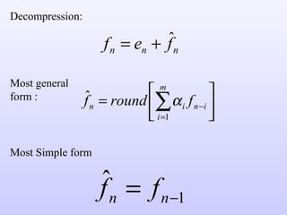
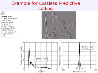
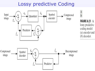
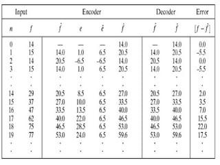
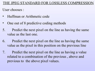
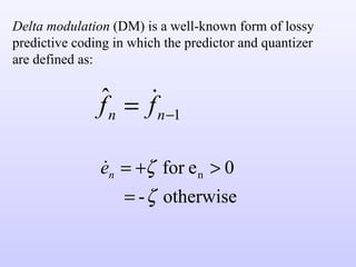
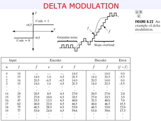
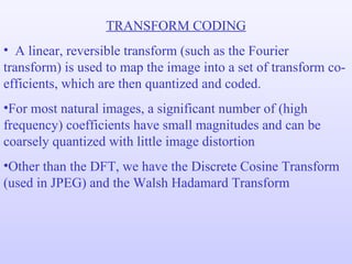
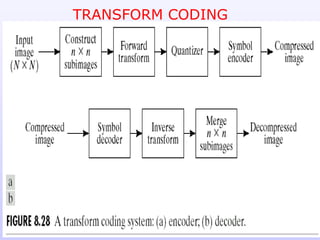
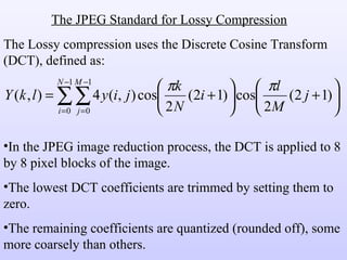
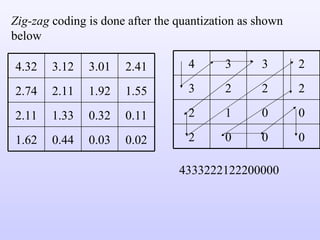
The document discusses various techniques for image compression including: 1) Variable length coding which reduces the first order entropy but not the second order entropy due to inter-pixel redundancy. 2) Predictive coding which codes only the difference between actual and predicted pixel values to remove inter-pixel redundancy. 3) Lossy compression techniques like transform coding and delta modulation which allow for higher compression ratios than lossless techniques by introducing some loss of information.

1. Using Information Theory: 21 21 21 95 169 243 243 243 21 21 21 95 169 243 243 243 21 21 21 95 169 243 243 243 21 21 21 95 169 243 243 243 First order entropy = 2*(3/8)*log 2 (8/3)+2*(1/8)*log 2 8 =1.81 bits/pixel Gray level Count Probability 21 12 3/8 95 4 1/8 169 4 1/8 243 12 3/8

2. Second-order entropy = 2*(1/4)*log 2 4+4*(1/8)*log 2 8=1+1.5=2.5 bits/pair = 1.25 bits/pixel. Gray level pair Count Probability (21,21) 8 ¼ (21,95) 4 1/8 (95,169) 4 1/8 (169,243) 4 1/8 (243,243) 8 ¼ (243,21) 4 1/8

3. The fact that the second order entropy (in bits/pixel) is less than the first order entropy, indicates the presence of inter-pixel redundancy. Hence variable length coding alone will not lead to the most optimum compression in this case. Consider mapping the pixels of the image to create the following representation: 21 0 0 74 74 74 0 0 21 0 0 74 74 74 0 0 21 0 0 74 74 74 0 0 21 0 0 74 74 74 0 0

4. Here, we construct a difference array by replicating the first column of the original image and using the arithmetic difference between adjacent columns for the remaining elements. First order entropy of this difference image = 1.41 bits/pixel Gray level or difference Count Probability 0 16 ½ 21 4 1/8 74 12 3/8

5. Near optimal variable length codes: Huffman codes require an enormous number of computations. For N source symbols, N-2 source reductions (sorting operations) and N-2 code assignments must be made. Sometimes we sacrifice coding efficiency for reducing the number of computations.

8. Truncated Huffman code: A truncated Huffman code is generated by Huffman coding only the most probable M symbols of the source, for some integer M (less than the total N symbols). A prefix code followed by a suitable fixed length is used to represent all other source symbols. In the table in the previous slide, M was arbitrarily selected as 12 and the prefix code was generated as the 13 th Huffman code word. That is a 13 th symbol whose probability is the sum of the probabilities of the symbols from 13 th to 21 st is included in the Huffman coding along with the first 12 symbols.

9. B-code: It is close to optimal when the source symbols probabilities obey a law of the form: P(a j ) = c j -   In the B-code, each code word is made up of continuation bits, denoted C, and information bits, which are binary numbers. The only purpose of the continuation bits is to separate individual code words, so they simply toggle between 0 and 1 for each new code word. The B-code shown here is called a B 2 code, because two information bits are used per continuation bit.

11. Shift code: A shift code is generated by Arranging the source symbols so that their probabilities are monotonically decreasing Dividing the total number of symbols into symbol blocks of equal size. Coding the individual elements within all blocks identically, and Adding special shift-up or shift-down symbols to identify each block. Each time a shift-up or shift-down symbol is recognized at the decoder, it moves one block up or down with respect to a pre-defined reference block.

12. Arithmetic coding: Unlike the variable-length codes described previously, arithmetic coding , generates non-block codes. In arithmetic coding, a one-to-one correspondence between source symbols and code words does not exist. Instead, an entire sequence of source symbols (or message) is assigned a single arithmetic code word. The code word itself defines an interval of real numbers between 0 and 1. As the number of symbols in the message increases, the interval used to represent it becomes smaller and the number of information units (say, bits) required to represent the interval becomes larger. Each symbol of the message reduces the size of the interval in accordance with the probability of occurrence. It is supposed to approach the limit set by entropy.

13. Arithmetic coding Let the message to be encoded be a 1 a 2 a 3 a 3 a 4

14. 0.2 0.4 0.8 0.04 0.08 0.16 0.048 0.056 0.072 0.0592 0.0624 0.0688 0.06368 0.06496

15. So, any number in the interval [0.06752,0.0688) , for example 0.068 can be used to represent the message. Here 3 decimal digits are used to represent the 5 symbol source message. This translates into 3/5 or 0.6 decimal digits per source symbol and compares favourably with the entropy of -(3x0.2log 10 0.2+0.4log 10 0.4) = 0.5786 digits per symbol

16. As the length of the sequence increases, the resulting arithmetic code approaches the bound set by entropy. In practice, the length fails to reach the lower bound, because : The addition of the end of message indicator that is needed to separate one message from another The use of finite precision arithmetic

17. 1.0 0.8 0.4 0.2 0.8 0.72 0.56 0.48 0.4 0.0 0.72 0.688 0.624 0.592 0.592 0.5856 0.5728 0.5664 Therefore, the message is a 3 a 3 a 1 a 2 a 4 0.5728 0.57152 056896 0.56768 Decoding: Decode 0.572. Since 0.8>code word > 0.4, the first symbol should be a 3 . 0.56 0.56 0.5664

18. LZW (Dictionary coding) LZW (Lempel-Ziv-Welch) coding, assigns fixed-length code words to variable length sequences of source symbols, but requires no a priori knowledge of the probability of the source symbols. The n th extension of a source can be coded with fewer average bits per symbol than the original source. LZW is used in: Tagged Image file format (TIFF) Graphic interchange format (GIF) Portable document format (PDF) LZW was formulated in 1984

19. The Algorithm: A codebook or “dictionary” containing the source symbols is constructed. For 8-bit monochrome images, the first 256 words of the dictionary are assigned to the gray levels 0-255 Remaining part of the dictionary is filled with sequences of the gray levels

20. Example: 39 39 126 126 39 39 126 126 39 39 126 126 39 39 126 126

22. Compression ratio = (8 x 16) / (10 x 9 ) = 64 / 45 = 1.4 Important features of LZW: The dictionary is created while the data are being encoded. So encoding can be done “on the fly” The dictionary need not be transmitted. Dictionary can be built up at receiving end “on the fly” If the dictionary “overflows” then we have to reinitialize the dictionary and add a bit to each one of the code words. Choosing a large dictionary size avoids overflow, but spoils compressions

23. Decoding LZW: Let the bit stream received be: 39 126 126 256 258 260 259 257 126 In LZW, the dictionary which was used for encoding need not be sent with the image. A separate dictionary is built by the decoder, on the “fly”, as it reads the received code words.

24. Recognized Encoded value pixels Dic. address Dic. entry 39 39 39 39 39 256 39-39 39 126 126 257 39-126 126 126 126 258 126-126 126 256 39-39 259 126-39 256 258 126-126 260 39-39-126 258 260 39-39-126 261 126-126-39 260 259 126-39 262 39-39-126-126 259 257 39-126 263 126-39-39 257 126 126 264 39-126-126

25. INTERPIXEL REDUNDANCY Variable length coding will produce identical compression ratios for the two images shown on the next slide, however we can achieve higher compression ratios by reducing interpixel redundancy. We can detect the presence of correlation between pixels (or interpixel redundancy) by computing the auto-correlation coefficients along a row of pixels

26. Maximum possible value of  n) is 1 and this value is approached for this image, both for adjacent pixels and also for pixels which are separated by 45 pixels (or multiples of 45).

27. Chapter 8 Image Compression

28. RUN-LENGTH CODING (1-D) Used for binary images Length of the sequences of “ones” & “zeroes” are detected. Assume that each row begins with a white(1) run. Additional compression is achieved by variable length-coding (Huffman coding) the run-lengths. Developed in 1950s and has become, along with its 2-D extensions, the standard approach in facsimile (FAX) coding.

29. Problems with run-length and LZW coding: Imperfect digitizing Vertical correlations are missed

31. An m-bit gray scale image can be converted into m binary images by bit-plane slicing. These individual images are then encoded using run-length coding. However, a small difference in the gray level of adjacent pixels can cause a disruption of the run of zeroes or ones. Eg: Let us say one pixel has a gray level of 127 and the next pixel has a gray level of 128. In binary: 127 = 01111111 & 128 = 10000000 Therefore a small change in gray level has decreased the run-lengths in all the bit-planes!

32. GRAY CODE Gray coded images are free of this problem which affects images which are in binary format. In gray code the representation of adjacent gray levels will differ only in one bit (unlike binary format where all the bits can change.

33. Let g m-1 …….g 1 g 0 represent the gray code representation of a binary number. Then: In gray code: 127 = 01000000 128 = 11000000

37. Decoding a gray coded image: The MSB is retained as such,i.e.,

38. Lossless Predictive Coding

39. Based on eliminating the interpixel redundancy in an image We extract and code only the new information in each pixel New information is defined as the difference between the actual ( f n ) and the predicted value, of that pixel.

40. Decompression: Most general form : Most Simple form

41. Example for Lossless Predictive coding

42. Lossy compression Lossless compression usually gives a maximum compression of 3:1 (for monochrome images) Lossy compression can give compression upto 100:1 (for recognizable monochrome images) 50:1 for virtually indistinguishable images The popular JPEG (Joint Photographic Experts Group) format uses lossy transform-based compression.

43. Lossy predictive Coding

44. Delta modulation (DM) is a well-known form of lossy predictive coding in which the predictor and quantizer are defined as:

45. DELTA MODULATION

47. TRANSFORM CODING A linear, reversible transform (such as the Fourier transform) is used to map the image into a set of transform co-efficients, which are then quantized and coded. For most natural images, a significant number of (high frequency) coefficients have small magnitudes and can be coarsely quantized with little image distortion Other than the DFT, we have the Discrete Cosine Transform (used in JPEG) and the Walsh Hadamard Transform

48. TRANSFORM CODING

49. THE JPEG STANDARD FOR LOSSLESS COMPRESSION User chooses : Huffman or Arithmetic code One out of 8 predictive coding methods Predict the next pixel on the line as having the same value as the last one. Predict the next pixel on the line as having the same value as the pixel in this position on the previous line Predict the next pixel on the line as having a value related to a combination of the previous , above and previous to the above pixel values.

50. The JPEG Standard for Lossy Compression The Lossy compression uses the Discrete Cosine Transform (DCT), defined as: In the JPEG image reduction process, the DCT is applied to 8 by 8 pixel blocks of the image. The lowest DCT coefficients are trimmed by setting them to zero. The remaining coefficients are quantized (rounded off), some more coarsely than others.

51. Zig-zag coding is done after the quantization as shown below 4333222122200000 4.32 3.12 3.01 2.41 2.74 2.11 1.92 1.55 2.11 1.33 0.32 0.11 1.62 0.44 0.03 0.02 0 0 0 2 0 0 1 2 2 2 2 3 2 3 3 4