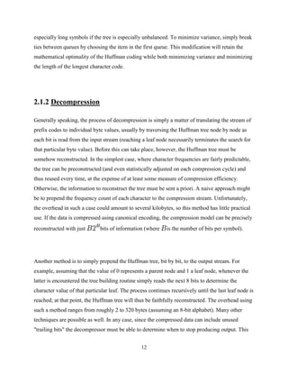
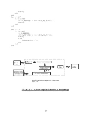
The document discusses image steganography and various related concepts. It introduces image steganography as hiding secret information in a cover image. Key points covered include: - Huffman coding is used to encode the secret image before embedding. It assigns binary codes to image intensity values. - Discrete wavelet transform (DWT) is applied to the cover image. The secret message is embedded in the high frequency DWT coefficients while preserving the low frequency coefficients to maintain image quality. - Inverse DWT is applied to produce a stego-image containing the hidden secret image. Haar DWT is used in the described approach.

1. 1
Chapter 1
Introduction

2. 2
1.1 Image Steganography
Image steganography[1][2]
is the art of hiding information into a cover image. Steganography is a
branch of information hiding in which secret information is camouflaged within other
information. The word steganography in Greek means “covered writing” ( Greek words “stegos”
meaning “cover” and “grafia” meaning “writing”) .
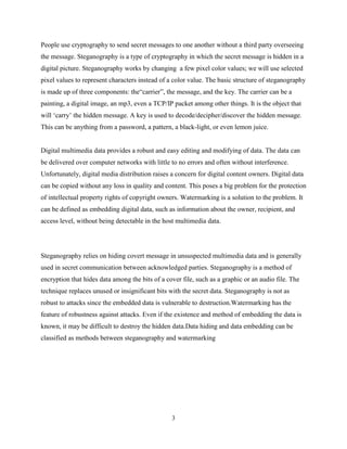
The main objective of steganography is to communicate securely in such a way that the true
message is not visible to the observer. That is unwanted parties should not be able to distinguish
any sense between cover-image (image not containing any secret message) and stego-image
(modified cover-image that containing secret message). Thus the stego-image should not deviate
much from original cover-image. Today steganography is mostly used on computers with digital
data being the carriers and networks being the high speed delivery channels. Figure. 1 shows the
block diagram of a simple image steganographic system.
FIGURE 1.1: The block diagram of a simple steganographic system

3. 3
People use cryptography to send secret messages to one another without a third party overseeing
the message. Steganography is a type of cryptography in which the secret message is hidden in a
digital picture. Steganography works by changing a few pixel color values; we will use selected
pixel values to represent characters instead of a color value. The basic structure of steganography
is made up of three components: the“carrier”, the message, and the key. The carrier can be a
painting, a digital image, an mp3, even a TCP/IP packet among other things. It is the object that
will ‘carry’ the hidden message. A key is used to decode/decipher/discover the hidden message.
This can be anything from a password, a pattern, a black-light, or even lemon juice.
Digital multimedia data provides a robust and easy editing and modifying of data. The data can
be delivered over computer networks with little to no errors and often without interference.
Unfortunately, digital media distribution raises a concern for digital content owners. Digital data
can be copied without any loss in quality and content. This poses a big problem for the protection
of intellectual property rights of copyright owners. Watermarking is a solution to the problem. It
can be defined as embedding digital data, such as information about the owner, recipient, and
access level, without being detectable in the host multimedia data.
Steganography relies on hiding covert message in unsuspected multimedia data and is generally
used in secret communication between acknowledged parties. Steganography is a method of
encryption that hides data among the bits of a cover file, such as a graphic or an audio file. The
technique replaces unused or insignificant bits with the secret data. Steganography is not as
robust to attacks since the embedded data is vulnerable to destruction.Watermarking has the
feature of robustness against attacks. Even if the existence and method of embedding the data is
known, it may be difficult to destroy the hidden data.Data hiding and data embedding can be
classified as methods between steganography and watermarking

4. 4
1.2 Types of Digital Images[5]
The Images types are :
1) Binary
2) Gray-Scale
3) Color
4) Multispectral
1.2.1 Binary Images
Binary images are the simplest type of images and can take on two values, typically black and
white, or 0 and 1. A binary image is referred to as a 1-bit image because it takes only 1 binary
digit to represent each pixel. These types of images are frequently used in applications where the
only information required is general shape or outline, for example optical character
recognititon(OCR).
Binary images are often created from the gray scale image via a threshold operation, where every
pixel above the threshold value is turned white(‘1’), and those below it are turned black(‘0’).
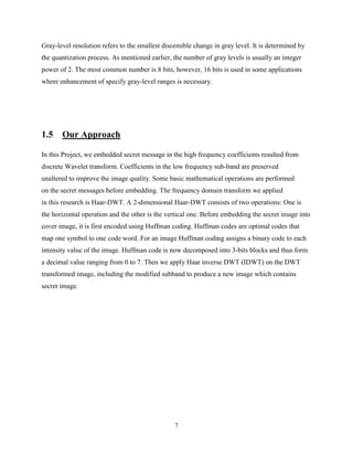
1.2.2 Gray-Scale Images
Gray-scale images are referred to as monochrome(one-color) images. They contain gray-level
information, no color information. The numbers of bits used for each pixel determines the
number of different gray levels available. The typical gray scale image contains 8 bits/pixel data,
which allows us to have 256 different gray levels.
In applications like medical imaging and astronomy, 12 or 16 bits/pixel images are used. These
extra gray levels become useful when a small section of the image is made much larger to
discern details.

5. 5
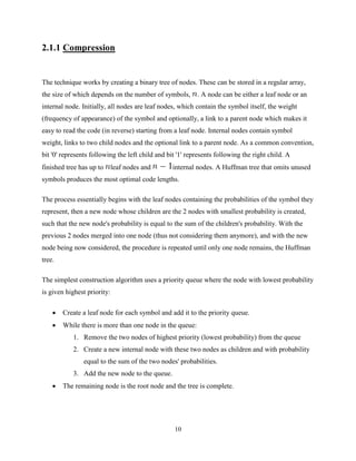
1.2.3 Color Images
Color images can be modeled as three-band monochrome image data, where each band of data
corresponds to a different color. The actual information stored in the digital image data is the
gray-level information in each spectral band.
Typical color images are represented as red, green, and blue(RGB images). Using the 8-bit
monochrome standard as a model, the corresponding color image would have 24 bits/pixel(8 bits
for each of the three color bands red, green, and blue).
1.2.4 Multispectral Images
Multispectral images typically contain information outside the normal human perceptual range.
This may include infrared, ultraviolet, X-ray, acoustic, or radar data. These are not images in the
usual sense because the information represented is not directly visible by the human system.
However, the information is often represented in visual form by mapping the different spectral
bands to RGB components.
1.3 Digital Image File Formats[5]
Types of image data divided into two primary categories : bitmap and vector.
 Bitmap images (also called raster images) can be represented as a 2-dimensional function
f(x,y), where they have pixel data and the corresponding gray-level values stored in some
file format.
 Vector images refer to methods of representing lines, curves, and shapes by storing only
the key points. These key points are sufficient to define the shapes. The process of
turning these into an image called rendering. After the image has been rendered, it can be
thought of as being in bitmap format, where each pixel has specific values associated
with it.

6. 6
Most of the types of file formats fall into the category of bitmap images, for example :
 PPM(Portable Pix Map) format
 TIFF(Tagged Image File Format)
 GIF(Graphics Image Format)
 JPEG(Joint Photographic Experts Group) format
 BMP(Windows Bitmap)
 PNG(Portable Network Graphics)
 XWD(X Window Dump)
1.4 Digital Image Representation[5]
The monochrome digital image f(x,y) resulted from sampling and quantization has finite discrete
coordinates (x,y) and intensities (gray levels). We shall use integer values for these discrete
coordinates, and gray levels. Thus, a monochrome digital image can be represented as a 2-
dimensional array (matrix) that has M rows and N columns. Each element of this matrix array is
called pixel. The spatial resolution (number of pixels) of the digital image is M*N. The gray
level resolution (number of gray levels) L is :
L=2k
Where k is the number of bits used to represent the gray levels of the digital image.
1.4.1 Spatial and Gray-level Resolution
Spatial resolution is the smallest discremble detail in an image.It is determined by the sampling
process.The spatial resolution of a digital image reflects the amount of details that one can see in
the image(i.e. the ratio of pixel “area” to the area of the image display). If an image is spatially
sampled at M*N pixels, then the larger M*N the finner the observed details.

7. 7
Gray-level resolution refers to the smallest discemible change in gray level. It is determined by
the quantization process. As mentioned earlier, the number of gray levels is usually an integer
power of 2. The most common number is 8 bits, however, 16 bits is used in some applications
where enhancement of specify gray-level ranges is necessary.
1.5 Our Approach
In this Project, we embedded secret message in the high frequency coefficients resulted from
discrete Wavelet transform. Coefficients in the low frequency sub-band are preserved
unaltered to improve the image quality. Some basic mathematical operations are performed
on the secret messages before embedding. The frequency domain transform we applied
in this research is Haar-DWT. A 2-dimensional Haar-DWT consists of two operations: One is
the horizontal operation and the other is the vertical one. Before embedding the secret image into
cover image, it is first encoded using Huffman coding. Huffman codes are optimal codes that
map one symbol to one code word. For an image Huffman coding assigns a binary code to each
intensity value of the image. Huffman code is now decomposed into 3-bits blocks and thus form
a decimal value ranging from 0 to 7. Then we apply Haar inverse DWT (IDWT) on the DWT
transformed image, including the modified subband to produce a new image which contains
secret image.

8. 8
Chapter 2
Elements of Design

9. 9
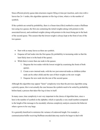
2.1 Huffman Coding[2][4]
Huffman coding is an entropy encoding algorithm used for lossless data compression. The term
refers to the use of a variable-length code table for encoding a source symbol (such as a character
in a file) where the variable-length code table has been derived in a particular way based on the
estimated probability of occurrence for each possible value of the source symbol.
Huffman coding uses a specific method for choosing the representation for each symbol,
resulting in a code that expresses the most common source symbols using shorter strings of bits
than are used for less common source symbols. no other mapping of individual source symbols
to unique strings of bits will produce a smaller average output size when the actual symbol
frequencies agree with those used to create the code. The running time of Huffman's method is
fairly efficient, it takes operations to construct it.
Although Huffman's original algorithm is optimal for a symbol-by-symbol coding (i.e. a stream
of unrelated symbols) with a known input probability distribution, it is not optimal when the
symbol-by-symbol restriction is dropped, or when the probability mass functions are unknown,
not identically distributed, or not independent (e.g., "cat" is more common than "cta").
FIGURE 2.1: The block diagram of Huffman Encoding

10. 10
2.1.1 Compression
The technique works by creating a binary tree of nodes. These can be stored in a regular array,
the size of which depends on the number of symbols, . A node can be either a leaf node or an
internal node. Initially, all nodes are leaf nodes, which contain the symbol itself, the weight
(frequency of appearance) of the symbol and optionally, a link to a parent node which makes it
easy to read the code (in reverse) starting from a leaf node. Internal nodes contain symbol
weight, links to two child nodes and the optional link to a parent node. As a common convention,
bit '0' represents following the left child and bit '1' represents following the right child. A
finished tree has up to leaf nodes and internal nodes. A Huffman tree that omits unused
symbols produces the most optimal code lengths.
The process essentially begins with the leaf nodes containing the probabilities of the symbol they
represent, then a new node whose children are the 2 nodes with smallest probability is created,
such that the new node's probability is equal to the sum of the children's probability. With the
previous 2 nodes merged into one node (thus not considering them anymore), and with the new
node being now considered, the procedure is repeated until only one node remains, the Huffman
tree.
The simplest construction algorithm uses a priority queue where the node with lowest probability
is given highest priority:
 Create a leaf node for each symbol and add it to the priority queue.
 While there is more than one node in the queue:
1. Remove the two nodes of highest priority (lowest probability) from the queue
2. Create a new internal node with these two nodes as children and with probability
equal to the sum of the two nodes' probabilities.
3. Add the new node to the queue.
 The remaining node is the root node and the tree is complete.

11. 11
Since efficient priority queue data structures require O(log n) time per insertion, and a tree with n
leaves has 2n−1 nodes, this algorithm operates in O(n log n) time, where n is the number of
symbols.
If the symbols are sorted by probability, there is a linear-time (O(n)) method to create a Huffman
tree using two queues, the first one containing the initial weights (along with pointers to the
associated leaves), and combined weights (along with pointers to the trees) being put in the back
of the second queue. This assures that the lowest weight is always kept at the front of one of the
two queues:
 Start with as many leaves as there are symbols.
 Enqueue all leaf nodes into the first queue (by probability in increasing order so that the
least likely item is in the head of the queue).
 While there is more than one node in the queues:
1. Dequeue the two nodes with the lowest weight by examining the fronts of both
queues.
2. Create a new internal node, with the two just-removed nodes as children (either
node can be either child) and the sum of their weights as the new weight.
3. Enqueue the new node into the rear of the second queue.
Although this algorithm may appear "faster" complexity-wise than the previous algorithm using
a priority queue, this is not actually the case because the symbols need to be sorted by probability
before-hand, a process that takes O(n log n) time in itself.
In many cases, time complexity is not very important in the choice of algorithm here, since n
here is the number of symbols in the alphabet, which is typically a very small number (compared
to the length of the message to be encoded); whereas complexity analysis concerns the behavior
when n grows to be very large.
It is generally beneficial to minimize the variance of codeword length. For example, a
communication buffer receiving Huffman-encoded data may need to be larger to deal with

12. 12
especially long symbols if the tree is especially unbalanced. To minimize variance, simply break
ties between queues by choosing the item in the first queue. This modification will retain the
mathematical optimality of the Huffman coding while both minimizing variance and minimizing
the length of the longest character code.
2.1.2 Decompression
Generally speaking, the process of decompression is simply a matter of translating the stream of
prefix codes to individual byte values, usually by traversing the Huffman tree node by node as
each bit is read from the input stream (reaching a leaf node necessarily terminates the search for
that particular byte value). Before this can take place, however, the Huffman tree must be
somehow reconstructed. In the simplest case, where character frequencies are fairly predictable,
the tree can be preconstructed (and even statistically adjusted on each compression cycle) and
thus reused every time, at the expense of at least some measure of compression efficiency.
Otherwise, the information to reconstruct the tree must be sent a priori. A naive approach might
be to prepend the frequency count of each character to the compression stream. Unfortunately,
the overhead in such a case could amount to several kilobytes, so this method has little practical
use. If the data is compressed using canonical encoding, the compression model can be precisely
reconstructed with just bits of information (where is the number of bits per symbol).
Another method is to simply prepend the Huffman tree, bit by bit, to the output stream. For
example, assuming that the value of 0 represents a parent node and 1 a leaf node, whenever the
latter is encountered the tree building routine simply reads the next 8 bits to determine the
character value of that particular leaf. The process continues recursively until the last leaf node is
reached; at that point, the Huffman tree will thus be faithfully reconstructed. The overhead using
such a method ranges from roughly 2 to 320 bytes (assuming an 8-bit alphabet). Many other
techniques are possible as well. In any case, since the compressed data can include unused
"trailing bits" the decompressor must be able to determine when to stop producing output. This

13. 13
can be accomplished by either transmitting the length of the decompressed data along with the
compression model or by defining a special code symbol to signify the end of input (the latter
method can adversely affect code length optimality, however).
2.1.3 Application
Arithmetic coding can be viewed as a generalization of Huffman coding, in the sense that they
produce the same output when every symbol has a probability of the form 1/2k
; in particular it
tends to offer significantly better compression for small alphabet sizes. Huffman coding
nevertheless remains in wide use because of its simplicity and high speed. Intuitively, arithmetic
coding can offer better compression than Huffman coding because its "code words" can have
effectively non-integer bit lengths, whereas code words in Huffman coding can only have an
integer number of bits. Therefore, there is an inefficiency in Huffman coding where a code word
of length k only optimally matches a symbol of probability 1/2k
and other probabilities are not
represented as optimally; whereas the code word length in arithmetic coding can be made to
exactly match the true probability of the symbol.
Huffman coding today is often used as a "back-end" to some other compression methods.
DEFLATE (PKZIP's algorithm) and multimedia codecs such as JPEG and MP3 have a front-end
model and quantization followed by Huffman coding (or variable-length prefix-free codes with a
similar structure, although perhaps not necessarily designed by using Huffman's algorithm.
2.2 Discrete Wavelet Transform[2][4]
In numerical analysis and functional analysis, a discrete wavelet transform (DWT) is any
wavelet transform for which the wavelets are discretely sampled. As with other wavelet
transforms, a key advantage it has over Fourier transforms is temporal resolution: it captures
both frequency and location information (location in time).

14. 14
2.2.1 Haar Wavelet
The first DWT was invented by the Hungarian mathematician Alfréd Haar. For an input
represented by a list of numbers, the Haar wavelet transform may be considered to simply
pair up input values, storing the difference and passing the sum. This process is repeated
recursively, pairing up the sums to provide the next scale: finally resulting in differences
and one final sum.
FIGURE 2.2: The block diagram of Discrete Wavelet Transform
2.2.2 Properties
The Haar DWT illustrates the desirable properties of wavelets in general. First, it can be
performed in operations; second, it captures not only a notion of the frequency content of the
input, by examining it at different scales, but also temporal content, i.e. the times at which these
frequencies occur. Combined, these two properties make the Fast wavelet transform (FWT) an
alternative to the conventional Fast Fourier Transform (FFT).

15. 15
2.2.3 Time Issues
Due to the rate-change operators in the filter bank, the discrete WT is not time-invariant but
actually very sensitive to the alignment of the signal in time. To address the time-varying
problem of wavelet transforms, Mallat and Zhong proposed a new algorithm for wavelet
representation of a signal, which is invariant to time shifts. According to this algorithm, which is
called a TI-DWT, only the scale parameter is sampled along the dyadic sequence 2^j (j∈Z) and
the wavelet transform is calculated for each point in time.
2.2.4 Application
The discrete wavelet transform has a huge number of applications in science, engineering,
mathematics and computer science. Most notably, it is used for signal coding, to represent a
discrete signal in a more redundant form, often as a preconditioning for data compression.
Practical applications can also be found in signal processing of accelerations for gait analysis,in
digital communications and many others.
It is shown that discrete wavelet transform (discrete in scale and shift, and continuous in time) is
successfully implemented as analog filter bank in biomedical signal processing for design of
low-power pacemakers and also in ultra-wideband (UWB) wireless communications.
FIGURE 2.3: The block diagram of Sub Bands

16. 16
2.3 Least Significant Bit Substitution
In computing, the least significant bit (lsb) is the bit position in a binary integer giving the units
value, that is, determining whether the number is even or odd. The lsb is sometimes referred to as
the right-most bit, due to the convention in positional notation of writing less significant digits
further to the right. It is analogous to the least significant digit of a decimal integer, which is the
digit in the ones (right-most) position.
It is common to assign each bit a position number, ranging from zero to N-1, where N is the
number of bits in the binary representation used. Normally, this is simply the exponent for the
corresponding bit weight in base-2 (such as in 231
..20
). Although a few CPU manufacturers
assign bit numbers the opposite way (which is not the same as different endianness), the term lsb
(of course) remains unambiguous as an alias for the unit bit.
By extension, the least significant bits (plural) are the bits of the number closest to, and
including, the lsb.
The least significant bits have the useful property of changing rapidly if the number changes
even slightly. For example, if 1 (binary 00000001) is added to 3 (binary 00000011), the result
will be 4 (binary 00000100) and three of the least significant bits will change (011 to 100). By
contrast, the three most significant bits stay unchanged (000 to 000).
Least significant bits are frequently employed in pseudorandom number generators, hash
functions and checksums.
2.4 Least Significant Byte
LSB (lsb) can also stand for least significant byte. The meaning is parallel to the above: it is the byte (or
octet) in that position of a multi-byte number which has the least potential value.

17. 17
Chapter 3
Software Implementation

18. 18
3.1 About Matlab
MATLAB[3]
(matrix laboratory) is a numerical computing environment and fourth-generation
programming language. Developed by Math Works, MATLAB allows matrix manipulations,
plotting of functions and data, implementation of algorithms, creation of user interfaces, and
interfacing with programs written in other languages, including C, C++, Java, and Fortran.
Although MATLAB is intended primarily for numerical computing, an optional toolbox uses
the MuPAD symbolic engine, allowing access to symbolic computing capabilities. An additional
package, Simulink, adds graphical multi-domain simulation and Model-Based
Design for dynamic and embedded systems.
In 2004, MATLAB had around one million users across industry and academia. MATLAB users
come from various backgrounds of engineering, science, and economics.
Syntax-The MATLAB application is built around the MATLAB language, and most use of
MATLAB involves typing MATLAB code into the Command Window (as an interactive
mathematical shell), or executing text files containing MATLAB codes, including scripts
and/or functions.
Variables-Variables are defined using the assignment operator, =. MATLAB is a weakly
typed programming language because types are implicitly converted. It is a dynamically typed
language because variables can be assigned without declaring their type, except if they are to be
treated as symbolic objects,[8]
and that their type can change. Values can come from constants,
from computation involving values of other variables, or from the output of a function.
Structures-MATLAB has structure data types.[10]
Since all variables in MATLAB are arrays, a
more adequate name is "structure array", where each element of the array has the same field
names. In addition, MATLAB supports dynamic field names[11]
(field look-ups by name, field
manipulations, etc.). Unfortunately, MATLAB JIT does not support MATLAB structures,
therefore just a simple bundling of various variables into a structure will come at a cost.

19. 19
3.2 MATLAB Codes
1. Code for converting image to Huffman code
clc;
clear all;
img=imread('Desert.jpg');
%converting RGB to grayscale image
%monochoromatic luminance method
img1=.2989*img(:,:,1)+.5870*img(:,:,2)+.1140*img(:,:,3);
%imshow(img1);
%creating histogram og image
hist=imhist(img1);
%imhist(img1);
symbol=0:255;
sum=0;
%finding probabilities of each symbols
for i=1:256
sum=sum+hist(i);
end
for i=1:256
prob(i)=double(hist(i))/sum;
end
%prob;
f=0;
for i=1:256
f=f+prob(i);
end
%f;
[dict,avglen] = huffmandict(symbol,prob);
[rows columns size]=size(img1);
pixels=rows*columns
img2=reshape(img1,1,pixels);
encode = huffmanenco(img2,dict);
%pilot image
pilot=imread('Koala.jpg');
pilot1=.2989*pilot(:,:,1)+.5870*pilot(:,:,2)+.1140*pilot(:,:,3);
f=1;
[cA,cH,cV,cD] = dwt2(pilot1,'haar');
h=1;
w=1;
for i=1:2:442651
b(w)=encode(i)*2+encode(i+1);
w=w+1;
end
for i=1:267
for k=1:400
cH1(i,k)=cH(i,k)-mod(cH(i,k),4)+b(h);

20. 20
h=h+1;
end
end
for i=1:267
for k=1:400
cV1(i,k)=cV(i,k)-mod(cV(i,k),4)+b(h);
h=h+1;
end
end
for i=1:267
for k=1:400
if(h<221326)
cD1(i,k)=cD(i,k)-mod(cD(i,k),4)+b(h);
h=h+1;
else
cD1(i,k)=cD(i,k);
end
end
end
FIGURE 3.1: The block diagram of Insertion of Secret Image

21. 21
2. Histogram
%histogram of image
clc;
clear all;
img=imread('Koala.jpg');
%converting RGB to grayscale image
%monochoromatic luminance method
img1=.2989*img(:,:,1)+.5870*img(:,:,2)+.1140*img(:,:,3);
%imshow(img1);
%creating histogram og image
hist=imhist(img1);
imhist(img1);
3. Pilot Image
%pilot image
%pilot=imread('Koala.jpg');
%pilot1=.2989*pilot(:,:,1)+.5870*pilot(:,:,2)+.1140*pilot(:,:,3);
%[cA,cH,cV,cD] = dwt2(pilot1,'haar');
for i=1:2:442652
b(f)=encode(i)*2+encode(i+1);
j=j+1;
end
4. Retrieval Image
p=1;
for i=1:267
for o=1:400
ret(p)=mod(cH1(i,o),4);
p=p+1;
end
end
for i=1:267
for o=1:400
ret(p)=mod(cV1(i,o),4);
p=p+1;
end

22. 22
end
for i=1:267
for o=1:400
if(p<=442652)
ret(p)=mod(cD1(i,o),4);
p=p+1;
else
break;
end
end
end
p=1;
for i=1:267
for o=1:400
ret(p)=mod(cH1(i,o),4);
p=p+1;
end
end
for i=1:267
for o=1:400
ret(p)=mod(cV1(i,o),4);
p=p+1;
end
end
for i=1:267
for o=1:400
if(p<=442652)
ret(p)=mod(cD1(i,o),4);
p=p+1;
else
break;
end
end
end
5. Huffmandict
clc;
clear all;
img=imread('Koala.jpg');
%converting RGB to grayscale image
%monochoromatic luminance method
img1=.2989*img(:,:,1)+.5870*img(:,:,2)+.1140*img(:,:,3);
%imshow(img1);
%creating histogram og image
hist=imhist(img1);
%imhist(img1);
symbol=[1:256];
sum=0;
%finding probabilities of each symbols

23. 23
for i=1:256
sum=sum+hist(i);
end
for i=1:256
prob(i)=double(hist(i))/sum;
end
%prob;
f=0;
for i=1:256
f=f+prob(i);
end
%f;
[dict,avglen] = huffmandict(symbol,prob);
6. Display
%reconstruction from modified subband
f=idwt2(cA,cH,cV,cD,'haar');
f1=idwt2(cA,cH1,cV1,cD1,'haar');
subplot(4,3,1);imshow(f,[]);title('Origanal Pilot Image')
subplot(4,3,4);imshow(cH);title('Origanal Vector Horizontal')
subplot(4,3,7);imshow(cV);title('Origanal Vector Vertical')
subplot(4,3,10);imshow(cD);title('Origanal Vector Diagonal')
subplot(4,3,3);imshow(f1,[]);title('Stegno Image')
subplot(4,3,6);imshow(cH1);title('Modified Vector Horizontal')
subplot(4,3,9);imshow(cV1);title('Modified Vector Vertical')
subplot(4,3,12);imshow(cD1);title('Modified Vector Diagonal')
subplot(4,3,5);imshow(img);title('Secret Image')

24. 24
Chapter 4
Results and Conclusion

25. 25
4.1 Result
The process of Image Steganography has been implemented by writing codes in MATLAB. The
brief study of MATLAB software has been done and various functions has been studied.
Huffman Coding and Discrete Wavelet transform has been studied and implemented.
4.2 Conclusion
Steganography is not intended to replace cryptography but rather to supplement it. If a message
is encrypted and hidden with a steganographic method it provides an additional layer of
protection and reduces the chance of the hidden message being detected.
Steganography is still a fairly new concept to the general public although this is likely not true in
the world of secrecy and espionage. Digital watermark technology is currently being used to
track the copyright and ownership of digital content. Efforts to improve the robustness of the
watermarks are necessary to ensure that the watermarks and embedded information can securely
defend against watermarking attacks.
With continuous advancements in technology it is expected that in the near future more efficient
and advanced techniques in steganalysis will emerge that will help law enforcement to better
detect illicit materials transmitted through the Internet.

26. 26
4.3 Future Scope
The most important application can be in the field of “Hacking”. Hacking is nothing but
unauthorised access of data which can be collected at the time of data transmission. This problem
is also known as Steganalysis. Steganography is a solution to above problem. A hopeful
advancement is the improved sensitivity to small message. Such a small file of few lines can be
aal that is needed to commence a terrorist attack. In future Steganalysis will advance such that it
will become much easier to detect even small messages.

27. 27
REFERENCES
1. Chen, P.Y. and Wu, W.E. “ A DWT Based Approach for Image Steganography ”,
International Journal of Applied Science and Engineering[1]
2. A Novel Technique for Image Steganography Based on DWT and Huffman Encoding by
Amitava Nag, Sushanta Biswas, Debasree Sarkar & Partha Pratim Sarkar[2]
3. Wikipedia - The Free Encyclopedia. Steganography.
http://en.wikipedia.org/wiki/Steganography[3]
4. Digital Image Processing Using MATLAB by Rafael C. Gonzalez and Steven L.
Eddins[4]
5. http://uotechnology.edu.iq/DIP_Lecture2.pdf[5]